Abstract
The Late Jurassic–Early Cretaceous (J3–K1) transboundary aquifer is the most important groundwater body in southern–southeastern Romania, shared with Bulgaria and hosted in karstic–fractured carbonates. We conducted an integrated evaluation of this aquifer by analyzing three 700 m deep groundwater exploration–exploitation boreholes, which intercepted it in the Cernavodă area (South Dobrogea region). The evaluation was based on geophysical wireline logging, drilling information, and borehole production tests. A K-means clustering of the logging data was performed for lithology typing, formation boundaries identification, and the delineation of probable producing intervals associated with secondary porosity development. Petrophysical interpretation was carried out via depth-constrained (zonal) inversion, using multimineral models, the estimated formation boundaries, and variable uncertainties for the main input logs. The optimal interpretation models were correlated with borehole testing results to gain insight into the hydrogeological properties of the aquifer complex. The fractured–vuggy interval with the highest water-producing potential was identified in the lower section of the J3-age Rasova Formation (639–700 m depth), comprising mainly undolomitized limestones. A southeast-to-northwest trend of increasing productivity of the boreholes, correlated with an increasing lateral dolomitization intensity within the Rasova Formation, suggests a highly heterogeneous character of the aquifer. The differences in productivity are due not only to local porosity variations but also to various degrees of pore space connectivity that are related to the amount of fracturing or karstification. The novel findings of this study have important practical implications for the optimal placement, design, and drilling program of future groundwater exploitation boreholes in the Cernavodă area and neighboring sectors.
1. Introduction
It is estimated that carbonate reservoirs—limestones and dolomites—host more than half of the world’s oil and gas reserves [1] and also much of the known groundwater reserves. With respect to clastic reservoirs rocks, carbonates often have a highly heterogeneous structure, leading to various petrophysical interpretation difficulties and to uncertainties in predicting reservoirs’ quality over larger scales [2,3,4]. Carbonate reservoirs are very frequently fractured and can have multiple pore sizes (microporosity to megaporosity) and also multiple porosity types: primary/“matrix” porosity (the interparticle pore space) and secondary porosity (joints, fissures, fractures, channels, isolated or connected vugs/voids), with the secondary porosity usually being more important than the primary one [1,2,3,4,5,6].
The relationships between porosity and permeability in carbonates often exhibit significantly greater variability compared to clastic reservoirs. Their permeability depends not only on the pore volume but also on the pore-size distribution [3,4,5,7]. In addition to fractures and fissures, the initial connectivity of carbonates can be greatly enhanced by diagenetic processes, like the dolomitization of limestones in the presence of magnesium-bearing waters. Occasionally, this process may increase the porosity by 12–13% [1,4], although other studies suggest that the initial porosity of pre-existing limestones may be preserved or even destroyed through dolomitization [8,9].
One of the most important aquifer systems in Romania is the deep groundwater body coded RODL06 (international designation EB088), which is hosted in a Late Jurassic–Early Cretaceous (J3–K1) carbonate complex of the karstic–fractured type [10,11,12,13,14,15,16,17,18]. This transboundary complex of Oxfordian–Barremian limestones and dolomites is developed in the southern and southeastern parts of Romania (the Wallachian and South Dobrogea sectors of the Moesian Platform) and in the entire northern part of Bulgaria. The exploited groundwater is used for domestic purposes/the drinking water supply, industry, and agriculture. South of the study area, in northeastern Bulgaria (Dobrich district), the J3–K1 aquifer has a geothermal character, with temperatures of 32–41 °C in Balchik, Cape Kaliakra, and Shabla areas, reaching even 45–52 °C in the Varna region and providing thermal energy for coastal resorts [13,14]. This groundwater body has a total area of 24,374 km2, out of which 11,340 km2 are within the Romanian territory, with approximately 4500 km2 in the South Dobrogea sector [12]. Its thickness gradually decreases from southwest towards the northeast and east, varying from over 1000 m to 200–400 m [10], and the aquifer is confined (under pressure) over most of South Dobrogea’s area except the zone adjacent to Danube River [11,15]. The general flow direction is from southwest to northeast, and the discharge occurs mainly north of the Constanţa port city, on the Black Sea coast [10]. Long-term isotopic monitoring studies conducted by Ţenu et al. [10,16,17,18] have identified the main recharge area in the Pre-Balkan Platform in Bulgaria. The hydraulic transmissivity of the aquifer varies from hundreds m2/day to over 150,000 m2/day.
Despite the significant number of wells that have been drilled for groundwater or geothermal water extraction from the J3–K1 aquifer and for monitoring the groundwater quality and quantity, there is a very limited amount of published data and research concerning the geophysical responses and petrophysical characteristics of the hosting carbonate reservoir, especially with regard to its hydrogeological properties. Given the potential, the great areal extension, and the importance of this aquifer on national and international scales, the present study aims to fill this significant knowledge gap.
We evaluate three deep groundwater exploration and exploitation boreholes from the Cernavodă town area (South Dobrogea region, Romania), which intercepted the J3–K1 complex and provided a better understanding of this regional and highly heterogeneous reservoir. The boreholes were drilled vertically to a depth of 700 m to supply with fresh water the Cernavodă nuclear power complex and its additional facilities (Figure 1). Besides geological analyses carried out on cores and cuttings samples (particularly for the first borehole), a geophysical wireline logging program was conducted for the identification of probable water-bearing intervals (vugs, caverns, and fractures/fissures), porosity evaluation, detailed lithological characterization, and the delineation of the main sedimentary formations in correlation with the general geological framework of South Dobrogea. The interpretation approach that we utilized is the depth-constrained (zonal) inversion of the logging datasets based on distinct multimineral models, using as a control the lithological information from drill cores and cuttings. To improve and facilitate the rock typing and separation of the geological complexes, in addition to correlation between boreholes, we performed a cluster analysis of the joint logging datasets via a nonhierarchical K-means algorithm [3,19,20,21,22]. Because the formation boundaries (tops) were known with higher certainty only in the first borehole drilled, we used the parallelization of the electrofacies (specific combinations of geophysical log responses) [23,24,25] that resulted from cluster analysis to identify these boundaries in the other boreholes.
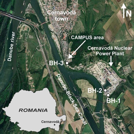
Figure 1.
Location of the analyzed groundwater exploration–exploitation boreholes (BH-1, BH-2, and BH-3) in the Cernavodă area, South Dobrogea region, Romania.
In this way, the geophysical logs inversion was depth-constrained in addition to the lithological controls to minimize the data fitting errors and optimize the interpretation models. Finally, the relationships between several parameters of the log interpretation models and the results of groundwater production tests are presented and discussed to highlight significant particularities of the analyzed aquifer complex, with practical implications upon the drilling of future groundwater extraction boreholes.
2. Geological and Tectonic Setting
The South Dobrogea Platform unit is situated in the southeastern part of the larger Dobrogean sector of the Moesian Platform. The unit is delimited by the NW–SE-trending Capidava–Ovidiu crustal fault (and the Central Dobrogea tectonic unit) to the north, the Black Sea shelf to the east, the NW–SE-trending Intramoesian crustal fault (and the Romania–Bulgaria state border as a formal boundary) to the south, and the NNE–SSW-trending Danube fault to the west [26,27].
The basement of the South Dobrogea unit consists of three metamorphic groups of the Archean to Late Proterozoic (Vendian) age. The overlying platform cover was deposited in five major marine transgression–regression cycles: Cambrian–Carboniferous, Permian–Triassic, Middle Jurassic–Late Cretaceous, Eocene–Oligocene, and Middle Miocene–Late Pliocene, alternating with exondation periods and followed by continental Quaternary sediments [26,27,28].
The Middle Jurassic–Late Cretaceous deposits, which host the J3–K1 groundwater body, are extended over the entire area of South Dobrogea and range in age from Bathonian to Santonian–Campanian. The Jurassic sequence comprises limestones, dolomitic limestones, and dolomites, with minor epiclastic intercalations. The Cretaceous sequence was formed in three stages: Berriasian to Barremian—evaporites and polychrome shales with extensions limited to the northern part of South Dobrogea, followed by shallow-marine shelf carbonates; Aptian—mostly continental fluvial and lacustrine deposits, with alteration products indicative of a tropical–subtropical climate, and subordinate clastics and carbonates developed in a marine littoral facies only in the western part of South Dobrogea; Albian to Senonian—clastic deposits, followed by chalk sedimentation [27,28].
The arrangement of Mesozoic and Cenozoic formations in South Dobrogea is complex, owing to the presence of numerous vertical and subvertical faults (Figure 2) [10,26,29]. These faults have divided the area into tectonic blocks that underwent either uplift or subsidence (Figure 3). The faulting events occurred after the accumulation of J3–K1 carbonate deposits and continued throughout the Cretaceous and Paleogene periods. Most of these blocks had ceased their movement before the deposition of Sarmatian (late Middle Miocene) formations, which exhibit a plate-like structure with an eastward inclination. The fault system with a WNW–ESE orientation (Cernavodă–Constanţa, Rasova–Costineşti, North Mangalia, and Mangalia faults) is newer, continuous, and runs parallel to the prominent Capidava–Ovidiu crustal fault [10,11,27]. These tectonic lineaments interact with an older fault system that is oriented NNE–SSW [10,11,27], resulting in the formation of 31 tectonic blocks of various sizes. The NNE–SSW fault system extends eastward into the continental shelf of the Black Sea.
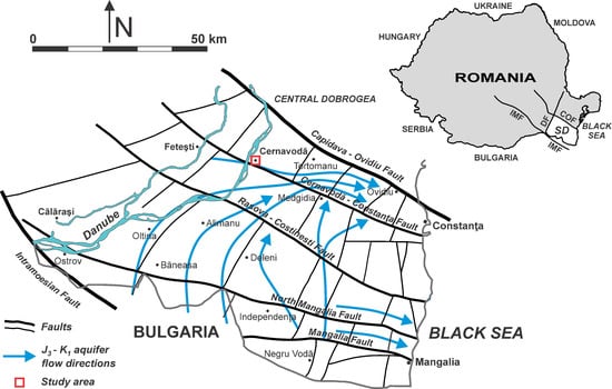
Figure 2.
Tectonic map of South Dobrogea (SD) showing the main fault systems and the general groundwater flow directions within the J3–K1 aquifer. COF—Capidava–Ovidiu fault, DF—Danube fault, IMF—Intramoesian fault (based on [10,29]).
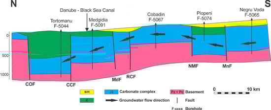
Figure 3.
Geological cross-section in N–S direction through South Dobrogea, illustrating the arrangement of tectonic blocks. COF—Capidava–Ovidiu fault, CCF—Cernavodă–Constanța fault, MdF—Medgidia fault, RCF—Rasova–Costinești fault, NMF—North Mangalia fault, MnF—Mangalia fault, sm—Sarmatian (prevailing oolitic limestones), K—Cretaceous (detrital and carbonates).
Previous geological studies based on outcrop samples and drill core data have shown that in the Cernavodă tectonic block, the Jurassic and Cretaceous formations are directly overlaid by Quaternary deposits. The following general lithostratigraphic succession has been outlined:
- (1)
- Quaternary—Holocene–Pleistocene loessoid deposits with paleosoils intercalations, which unconformably cover the Cretaceous formations. Usually, a 2–3 m thick level of reddish shales and reworked gravels (early Pleistocene) is present at the base of these loessoid deposits. The thickness of the Quaternary deposits ranges from 10 to 45 m.
- (2)
- Gherghina Formation—Middle–Late Aptian [30,31]. Continental fluvial–lacustrine deposits of 5–30 m thickness, consisting of polychrome kaolinitic shales with calcareous concretions in the upper part and sands, gravels, and conglomerates with a reddish shaly or silty matrix at the base of the unit. The continental deposits may change laterally and/or vertically into shallow marine facies with marlstones, siltstones, and sandstones with marly intercalations.
- (3)
- Cernavodă Formation—late Berriasian–Valanginian [30,31,32,33]. A shallow marine calcareous unit of 20–40 m thickness, discordantly overlaid by the Gherghina Formation and separated into two subunits in the study area: (a) the Aliman Member (Valanginian) at the upper part, unconformable and transgressive, consisting of calcirudites and calcarenites with numerous macro– and microfossils and intercalations of algal stromatolites; (b) the Hinog Member (late Berriasian) at the base, comprising conglomerates, sandy shales, argillaceous limestones, oolitic limestones, and biostromes, with gastropod fauna.
- (4)
- Amara Formation—Late Jurassic (late Tithonian)–Early Cretaceous (early–middle Berriasian) [31,33]. This unit of over 300 m thickness includes siliciclastic, carbonate, and evaporitic deposits and comprises two subunits in the study area: (a) the Zăvoaia Member (early–middle Berriasian) at the upper part, consisting of a 40–60 m thickness sequence of polychrome (reddish-violet, greenish) shales, marlstones, and oolitic and micritic limestones, overlying a marine carbonate sequence of up to 50–60 m thickness, which includes bioclastic limestones, detrital limestones, oolitic limestones, and calcareous sandstones, with intercalations of marlstones and argillaceous limestones. The rich fossil microfauna and microflora collected from the upper part of the Zăvoaia Member indicates a deposition in a continental–lacustrine and lagoonal, even littoral, environment and allowed a parallelization with the Purbeckian facies; (b) the Cireșu Member, representing an evaporitic sequence of 180–200 m thickness, consisting of massive gypsum and anhydrite, with intercalations of gypsiferous shales and marlstones, oolites, and micritic limestones of variable thicknesses. Secondary gypsum frequently appears deposited in the fissures or the bedding planes of the argillaceous rocks, and the gypsiferous shales adjacent to massive gypsum intervals show microfolds related to the hydration of anhydrite. The very scarce fossil microfauna are limited to species adapted to hypersaline conditions. This sequence is indicative of a lagoonal depositional environment in a warm and arid climate.
- (5)
- Rasova Formation (Oxfordian–Tithonian) [31,33]. The unit has a thickness of over 500 m and consists of dolomites (dolomicrites, dolosparites), dolomitic limestones, micritic limestones, and oosparites, with scarce fossil macro- and microfauna. Locally, the dolomites have a laminated appearance, with gray–yellowish bands alternating with greenish bands of more intense dolomitization. Marlstones, argillaceous limestones, and calcareous breccia levels appear as intercalations. Fractures/fissures and karstic dissolution voids are very frequent in this carbonate sequence, together with a porosity related to the dolomitization of limestones. These voids can be small and uniformly distributed or larger and irregular, forming channel systems. Likely, this occurs on a large scale, leading to an extended karst network within the Late Jurassic carbonates.
3. Borehole Data
The 700 m deep groundwater exploration–exploitation boreholes analyzed in this study, denoted BH-1, BH-2, and BH-3, were drilled within the site of the Cernavodă nuclear power complex (BH-1, BH-2) and in the Campus residential district of Cernavodă town (BH-3), on the northern bank of the Danube–Black Sea Canal. The distance between BH-1 and BH-2 is 203 m and the distance between BH-2 and BH-3 is 1645 m. The drilling with fresh water-based fluids and the geophysical investigation were carried out by the Romanian company Foradex S.A.—București (now Foraj București S.A.). The diameters of the intermediate and final sections of the boreholes are 12.25 in. and 8.5 in., respectively.
3.1. Geological Investigations
The BH-1 borehole provided the most complete information about the crossed geological sequence, based on lithological–petrographic and micropaleontogical analyses performed on extracted drill cores (60 m total core recovery) and drill cuttings (over 600 samples). For BH-2 and BH-3, fewer drill cuttings were available, resulting in uncertainties regarding the boundaries between the main geological formations. The laboratory analyses results obtained for BH-1 allowed the synthetic lithostratigraphy of the deposits from Cernavodă drilling sites area to be established. Certain units were assigned unconventional terminology, but they were correlated with the known general lithostratigraphic succession.
Based on drilling data analyses, the geological succession of the Cernavodă section crossed by the BH-1 borehole was reported as follows:
Quaternary Continental Deposits (“Q”): 0–25 m
Loess deposits, overlying rock debris with altered limestone fragments (Berriasian–Valanginian), and reworked elements from the underlying Aptian gravels. At the base of the debris layer, there are shales and sandy shales with freshwater lacustrine fauna.
Early Cretaceous Continental Deposits (“CD”): 25–30 m
Quartz sands and gravels, with intercalations of kaolinitic shales. The microfossil content indicates a Middle–Late Aptian age, and these deposits were considered to represent the Gherghina Formation.
Carbonate Complex I (“CC-I”): 30–45 m
The deposits consist primarily of carbonates and include bioclastic limestones with recrystallizations, detrital limestones, oolitic limestones, argillaceous limestones, marlstones, and calcareous sandstones. The rich marine microfauna suggest a late Berriasian–early Valanginian age. This carbonate complex was assigned to the Cernavodă Formation.
Polychrome Marlstones and Shales Complex (“PMSC”): 45–100 m
Greenish or violet marlstones and shales with intercalations of detrital limestones, calcareous sandstones, oolites, argillaceous limestones, and silty shales. They contain rich brackish and freshwater microfauna of an early–middle Berriasian age, characteristic for the Purbeckian facies. This mainly argillaceous complex was assigned to the upper part of the Zăvoaia Member—Amara Formation.
Carbonate Complex II (“CC-II”): 100–161 m
Predominantly bioclastic limestones, oolites, argillaceous limestones, and marlstones. The abundant marine-type microfauna collected from this carbonate sequence indicate an early Berriasian age, and the complex is considered the lower part of the Zăvoaia Member—Amara Formation.
Evaporite Complex (“EC”): 161–363 m
Gypsum and anhydrite, gypsiferous shales, and marlstones, with thin intercalations of oolites and argillaceous limestones. The very sparse microfauna encountered are representative for the late Tithonian age, and this complex was assigned to the basal Cireșu Member—Amara Formation.
Dolomite Complex (“DC”): 363–700 m
Dolomites, limestones partially affected by dolomitization, hard micritic limestones, and thin intercalations of marlstones or argillaceous limestones. The process of dolomitization of the pre-existing limestones is not uniform, as it is more intense in the upper part of the complex. The scarce microfossil content indicates a Kimmeridgian–early-to-middle Tithonian age. The Dolomite Complex corresponds to the Rasova Formation and represents the main exploration objective of the analyzed boreholes.
3.2. Geophysical Investigation Program
The phases of the open-hole wireline logging program carried out in the Cernavodă groundwater exploration boreholes are presented in Table 1. The investigation was performed using Robertson Geologging equipment and included conventional (standard) electrical logs, nuclear logs—total gamma ray and dual-spacing (compensated) thermal neutron, compensated sonic velocity logs, caliper, and borehole temperature logs. The main recorded curves (channels), at a depth sampling step of 0.1 m, are presented in Table 2. Not all logs were acquired over the entire depth of the boreholes.

Table 1.
Phases of the geophysical investigation program carried out in the groundwater exploration boreholes drilled in Cernavodă town area.
Table 2.
Geophysical well logs recorded in the groundwater exploration boreholes drilled in Cernavodă town area.
The nuclear log data were provided in counts per second (cps), so for the Dual Neutron tool only the short-spaced (Near detector) and long-spaced (Far detector) raw count rates were available, instead of a neutron porosity curve. The total gamma ray logs, though not expressed in standard American Petroleum Institute (API) units, are still adequate for the delineation of lithological complexes, clay volume estimation, and multimineral petrophysical interpretation. The unfocused Electric Log tool employed for the resistivity logging had an operating range of 1–10,000 Ω m, but is not ideally suited for the investigation of high-resistivity carbonate formations, as ρA,16 and ρA,64 measurements are sometimes adversely affected by the borehole influence (diameter variations, mud resistivity). A focused resistivity logging device (Laterolog/Guard Log type) was not available for the investigations.
The data channels were edited to remove invalid start and end readings, a five-point (0.5 m) moving average smoothing filter was applied to the nuclear logs, and single composite logs were created through the optimal splicing (merging) of the individual segments recorded over different depth intervals (Figure 4, Figure 5 and Figure 6). Due to the limited quantitative usefulness of the SP in carbonate formations and the uncertainty of baseline shifts over the borehole sections drilled in different stages, the SP log segments were not merged.
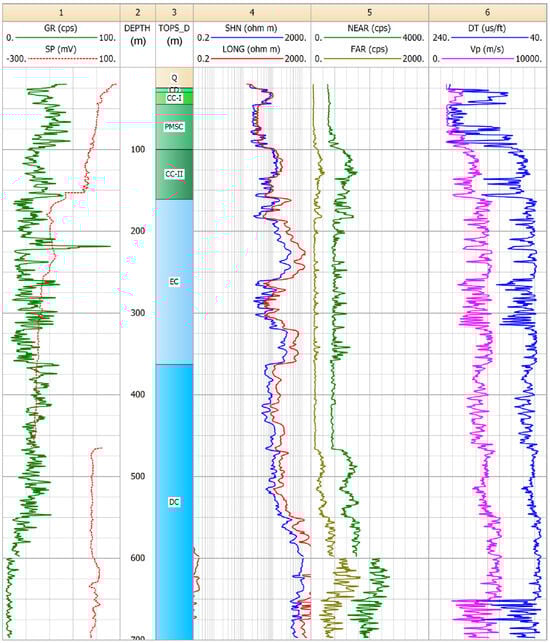
Figure 4.
Geophysical wireline logs recorded in BH-1 borehole: track 1—total gamma ray(cps) and SP (mV); track 2—measured depth (m); track 3 (TOPS_D)—formation boundaries (tops) reported from drilling data and geological analyses (m); track 4—short normal and long normal apparent resistivities [Ω m]; track 5—short-spacing and long-spacing neutron count rates (cps); track 6—compensated sonic interval transit time (μs/ft) and P-wave velocity (m/s). Caliper log and borehole temperature data were not available for BH-1.
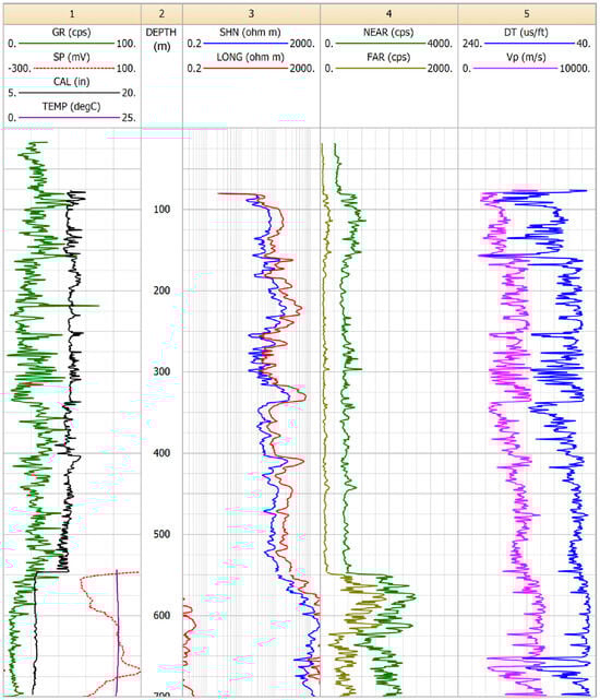
Figure 5.
Geophysical wireline logs recorded in BH-2 borehole: track 1—total gamma ray (cps), SP (mV), caliper (in), and borehole temperature (°C); track 2—measured depth (m); track 3—short normal and long normal apparent resistivities (Ω m); track 4—short-spacing and long-spacing neutron count rates (cps); track 5—compensated sonic interval transit time (μs/ft) and P-wave velocity (m/s). Note the change in borehole diameter at 546 m depth.
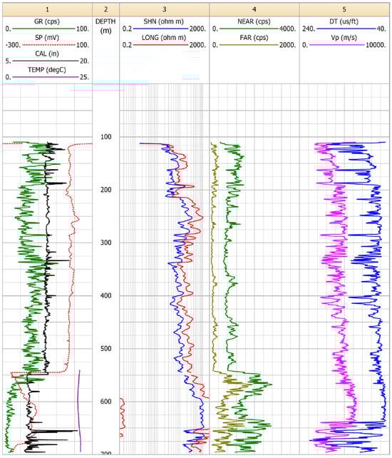
Figure 6.
Geophysical wireline logs recorded in BH-3 borehole: track 1—total gamma ray (cps), SP (mV), caliper (in), and borehole temperature (°C); track 2—measured depth (m); track 3—short normal and long normal apparent resistivities (Ω m); track 4—short-spacing and long-spacing neutron count rates (cps); track 5—compensated sonic interval transit time (μs/ft) and P-wave velocity (m/s). Note the change in borehole diameter at 549 m depth.
4. Data Processing and Interpretation
The wireline logs recorded in the BH-1, BH-2, and BH3 boreholes were processed and interpreted to achieve the following goals: (a) porosity evaluation from the neutron and sonic logs to assess the most appropriate sonic porosity transform and to identify the intervals with significant secondary porosity, i.e., the potential water-producing horizons; (b) correlation of the main geological formations (complexes) between the boreholes and an improved delineation of the formation boundaries using multivariate statistical classification via cluster analysis; (c) depth-constrained logging data inversion based on optimal multimineral models, for a comprehensive evaluation of the formations lithology, true porosity, and groundwater resistivity/salinity.
The multivariate analyses and the logging data inversion were conducted over the intervals with complete log coverage: 25–697 m in BH-1, 80–698 m in BH-2, and 112–696 m in BH3.
4.1. Neutron Porosity Evaluation
The dual-detector neutron tool significantly reduces the adverse borehole effects, and the ratio of count rates between the detectors (Ratio = In,Far/In,Near) is proportional to the neutron (apparent) porosity ϕN, i.e., the formation hydrogen index. The primary calibration of the tool (experimentally derived relations between the counts ratio and the decimal logarithm of ϕN relative to a limestone matrix) was performed by the manufacturing company in water-filled boreholes with standard diameters. The calibration transforms Ratio [dec.] → ϕN [%] were provided as sets of coefficients of the polynomial Equation (1)
with a, b, c, and d taking particular values for each reference borehole diameter. We have elaborated and utilized a MATLAB code to compute the limestone-based ϕN (NPHI curves) for arbitrary borehole diameters, provided by the CAL curve, through interpolation between the reference ϕN values calculated with Equation (1). In carbonate formations, ϕN corresponds to the total porosity (ϕt), i.e., the sum of the primary (interparticle) and secondary (vug and fracture) porosities. The code for ϕN computation is presented in Appendix A.
ϕN(Ratio) = a + b Ratio + c Ratio2 + d Ratio3
4.2. Sonic (Acoustic) Porosity Evaluation
The sonic porosity (ϕS) was computed using the Raymer et al. [34] transit time–porosity transform and the Raiga-Clemenceau et al. [35] acoustic formation factor equation, assuming a limestone lithology as a reference. The resulting ϕS (SPHI curves in Figure 7 and Figure 8) were evaluated by comparison with the computed limestone neutron porosity ϕN.
The empirical Raymer et al. transform operates over the entire porosity range. For the lower (0 to 0.37) and upper (0.47 to 1) ranges, ϕ (i.e., ϕS) results from Equations (2) and (3)
where Δt1 and Δt2 are measured or predicted P-wave transit times; ϕ is the fractional porosity, δ is the bulk density of the formations; Δtma and δma are the P-wave transit time and the density of the rock matrix; and Δtf and δf are the P-wave transit time and the density of the pore fluid (mud filtrate). The commonly adopted parameter values are Δtma = 56 μs/ft and δma = 2.65 g/cm3 for quartz sands/sandstones; Δtma = 49 μs/ft and δma = 2.71 g/cm3 for limestones; Δtma = 44 μs/ft and δma = 2.86 g/cm3 for dolomites; Δtf = 189 μs/ft and δf = 1.0 g/cm3 for freshwater mud filtrate; and Δtf = 185 μs/ft and δf = 1.1 g/cm3 for saltwater mud filtrate [6,7,34,36].
For the intermediate porosity range (0.37 to 0.47), a linear interpolation between Δt1 and Δt2 is used—Equation (4) or the simplified Equation (5):
Equations (2) and (5) allow for the estimation of sonic porosities of up to 0.47 without density log data, which were not available in the analyzed boreholes.
The Raiga-Clemenceau et al. transit time–porosity transform is given by
The sonic porosity is obtained from the measured Δt:
where x is a lithology-dependent exponent. The parameters in Equations (6) and (7) for the typical reservoir lithologies are Δtma = 55.5 μs/ft and x = 1.60 for quartz sands/sandstones; Δtma = 47.6 μs/ft and x = 1.76 for limestones; and Δtma = 43.5 μs/ft and x = 2.00 for dolomites.
4.3. Cluster Analysis
For the multivariate cluster analysis of the wireline logging datasets, we used an unsupervised K-means algorithm [19,20,21,22] to assign individual data points to electrofacies of physical properties, which could be correlated to the main geological formations (lithologies) or to specific geological facies [23,24,25]. The number of clusters (K) utilized for partitioning the data is user-imposed. The algorithm partitions a set of N data points into distinct K domains (K < N) so that the data dispersion within each domain is minimal, i.e., the data are as “similar” as possible. The steps involved in the cluster analysis are as follows:
- Define the number of clusters;
- Randomly initialize the cluster centroids (seed points);
- Assign data points to the cluster with the closest centroid;
- Recalculate the cluster centroids based on the data in each cluster;
- Repeat steps 3 and 4 until convergence is achieved, i.e., the cluster centroids stabilize and the allocation of data points to clusters remains unchanged.
The clustering solution is obtained by iteratively minimizing the objective function F from Equation (8), which represents the total within-cluster variation (the sum of squared distances between the data points and the related centroid given by Equation (9))
where xi is a data point, Cj is a current cluster, μj is the mean value assigned to cluster Cj (the centroid of the cluster), and nj is the number of data points in cluster Cj. The logging data were standardized (normalized) before clustering by subtracting the mean and dividing by the standard deviation of each log to ensure a consistent range for all the logs. The ρA input data were represented by the decimal logarithm of the SHN and LONG curves.
To determine the appropriate number of clusters, we performed a preliminary multiborehole analysis by simultaneously utilizing all the logging datasets (GR, SHN, LONG, NPHI, and DT curves) with a relatively large value of K (K = 10). We defined cluster randomness through the ratio ha/hr [37,38], where ha is the average thickness of a cluster layer, i.e., the average number of depth levels per cluster, and hr is the theoretical average random thickness of a layer, calculated assuming the clusters to be assigned randomly at each depth level. The hr is given by
where pj is the proportion of depth levels assigned to the j-th cluster [37,38]. Higher values of the ratio correspond to less random clusters, i.e., more structured logging data. We employed the plot of cluster randomness ratio as a function of the number of clusters and identified a likely range for K around the inflection point where the ratio ceased to decrease significantly.
4.4. Quantitative Log Interpretation
The interpretation of the wireline logging datasets was carried out with a probabilistic inversion algorithm included in the Mineral Solver module from the Interactive Petrophysics™ (version 4.6) log analysis software [38]. The algorithm solves for mineralogy, porosity, and fluid saturations by considering the linearized response equations of the logging tools, the volumetric endpoint parameters (theoretical logging tools responses for 100% content of a particular mineral or fluid), and the likely uncertainties associated with the measured logs.
Given a set of m measured logs X1, X2, …, Xm and a petrophysical interpretation model V = [V1, V2, …, Vp] with p parameters (the unknown solid and fluid volume fractions of the formations), the optimal solution vector is obtained by iteratively minimizing the normalized fitting error E(V) from Equation (11)
where L1, L2, …, Lm are theoretical (reconstructed) log responses corresponding to a particular model vector in an arbitrary iteration and σ1, σ2, …, σm are user-defined uncertainties (confidence weights) associated with the measured logs. Smaller σ values imply a high degree of confidence (accurate log readings, good borehole conditions) and a higher weighting factor for a particular log response equation, whereas larger σ values stand for a decreased confidence (errors affecting the logs, poor borehole conditions) and a lower weighting factor.
A volumetric constraint (unity equation) V1 + V2 + … + Vp = 1 is imposed for the components of the solution vector, as well as physical constraints like 0 ≤ Vk ≤ 1, k = 1,…, p. Starting with an approximate solution V(0) = [V1(0), V2(0), …, Vp(0)], the inversion algorithm computes a series of model correction vectors ΔV = [ΔV1, ΔV2, …, ΔVp] in each iteration and updates the current model, i.e., V = V(0) + ΔV. The model optimization continues until the data misfit (14) is minimized and convergence is reached (the computed solid and fluid volume fractions do not change significantly between iterations). We used a general interpretation model V = [Vquartz, Vcalcite, Vdolomite, Vgypsum, Vanhydrite, Vclay, Vwater = ϕ], where the particular components of V at each level are depth-zoned according to the identified formation boundaries.
As main inputs for the inversion algorithm, we utilized the GR, DT, and NPHI curves to evaluate the clay volume, porosity, lithology, and LONG curves—approximating the true resistivity of the water-saturated formations ρo—to estimate water resistivity (ρw) and calibrate the water saturation (Sw) to unity in the porous permeable aquifer sections. The Poupon–Leveaux (“Indonesia”) [3,39] model was used for Sw computation, with a saturation exponent set to n = 2. Generic values suitable for carbonates a = 1 and m = 2 were used for the tortuosity factor and the cementation exponent in the formation factor F expression (12) [6,7,40]:
The adopted m = 2 average cementation exponent balances the characteristic values for fractured carbonates (average m = 1.4) with those representative for vuggy (m = 2.1–2.6) or moldic porosity (m ≥ 3.0) [1,41].
We derived the probable ρw (and thereby the water salinity) by computing synthetic resistivity logs corresponding to water-saturated formations, i.e., ρo = a/ϕm ρw. The ρw values were adjusted until Sw ≈ 1, and a match between the ρo logs and the measured ρA,64 logs was obtained in the reservoir intervals. The average wet clay parameters necessary for porosity–lithology evaluation and Sw correction in the shalier intervals were estimated statistically from multiborehole (joint wireline logging datasets) histograms and crossplots: Iγ,clay = 90 cps, ϕN,clay = 0.40–0.45, Δtclay = 90–110 μs/ft, and ρclay = 20 Ω m. The background gamma ray radioactivity corresponding to the cleanest carbonate sections was selected: Iγ,clean = 5 cps. We employed the following matrix and fluid (mud filtrate) parameters for the neutron and sonic logs: ϕN,quartz = −0.02, ϕN,calcite = 0, ϕN,dolomite = 0.01, ϕN,gypsum = 0.6, ϕN,anhydrite = −0.02, Δtquartz = 55.5 μs/ft, Δtcalcite = 47.6 μs/ft, Δtdolomite = 43.5 μs/ft, Δtgypsum = 52 μs/ft, Δtanhydrite = 50 μs/ft, ϕN,fluid = 1, and Δtfluid = 189 μs/ft [6,32]. For the lithology–porosity logs, on the intervals with good hole conditions and a sonic response unaffected by attenuation (abnormally high Δt values), we used σGR = 5 cps, σNPHI = 0.02, and σDT = 3 μs/ft as default uncertainties.
5. Results and Discussion
5.1. Quick-Look Analysis
A common feature observed on the BHC (Borehole Compensated Sonic) logs from the analyzed Cernavodă boreholes is represented by abnormally high compressional transit time readings at certain depths, with Δt reaching 210–220 μs/ft and exceeding the mud filtrate transit time (Figure 4, Figure 5 and Figure 6). Within the carbonate formations, especially in the final 8.5 in. borehole sections within the Dolomite Complex (≈635–700 m depth), we attribute this to a cycle-skipping effect caused by the P-wave attenuation in horizontal–inclined fractures/fissures or in karstified zones with a vuggy porosity [6]. In this case, the first arrival of the P-wave is too weak to trigger the receivers of the sonic tool, which record only later arrivals of higher amplitudes.
Correlated with the very high Δt values, additional indications for the presence of fractures or fluid-filled caverns in the lower part of the Dolomite Complex are (a) significant increases in the borehole diameter (up to 18 in.) on several depth intervals, as seen on the CAL log from BH-3; (b) strong decreases in the recorded ρA values, from 1200–2000 Ω m (SHN curves) or 3100–4700 Ω m (LONG curves) in the most compact carbonate intervals to 100–400 Ω m (SHN curves) or 300–900 Ω m (LONG curves); (c) local increases in the computed ϕN values, from about 0.03 in the tightest intervals to 0.22–0.23 (BH-1 and BH-2 boreholes) and up to 0.44 (BH-3 borehole).
Figure 7 shows the frequency distribution (stacked histograms) of the sonic porosities computed using the Raymer et al. and the Raiga-Clemenceau et al. Δt→ϕS transforms, assuming a standard limestone matrix. Additionally, the frequency distribution of computed limestone ϕN values is included for comparison.
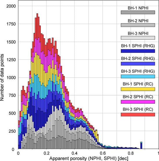
Figure 7.
Stacked histograms of the computed neutron (NPHI) and sonic (SPHI) apparent porosities referenced to a limestone matrix for the Cernavodă boreholes (25–698 m overall depth interval). RHG—Raymer–Hunt–Gardner sonic porosity transform, RC—Raiga-Clemenceau sonic porosity transform.
It is evident that the range of ϕS variation derived from the Raiga-Clemenceau et al. transform better matches the ϕN range for all the analyzed boreholes, whereas the Raymer et al. transform occasionally leads to unrealistically high ϕS values. Considering that Equations (6) and (7) are also independent of Δtf (a common source of uncertainty), we have selected the Raiga-Clemenceau et al. transform as the most suitable for ϕS evaluation in the studied boreholes and, in addition, as the sonic log response equation in the logging data inversion algorithm.
Figure 8 (tracks 3, 4, and 5) displays an overlay of the ϕN and ϕS apparent porosity curves computed for a standard limestone matrix. For reference, the BH-1 borehole formation boundaries as reported from cores and cuttings analyses are shown in track 2.
For all boreholes, the superposition of ϕN and ϕS in various depth intervals within the Cretaceous deposits and the Dolomite Complex indicates mostly clean limestones with primary porosity and validates the utilized In,Far/In,Near→ϕN and Δt→ϕS transforms. The Evaporite Complex is clearly delineated by very large separations ϕN > ϕS exceeding 0.50 (ϕN − ϕS ≥ 50% equivalent limestone porosity), due to the neutron log response to the crystallization water of gypsum. In the carbonate formations, especially near the boreholes’ terminal depth within the Dolomite Complex, large inverse separations ϕS > ϕN (ϕS − ϕN = 0.30–0.43) are diagnostic for intervals with a fluid-filled secondary porosity (karstic dissolution voids or fractures). This effect appears more significant in the BH-3 borehole (below 638 m depth) and of lesser magnitude in BH-1 and BH-2 (below 651 m depth).
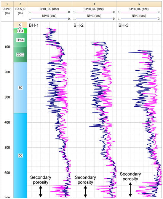
Figure 8.
Overlay of neutron (NPHI curves) and sonic (SPHI_RC curves—Raiga-Clemenceau transform) apparent porosities computed assuming a standard limestone matrix for the Cernavodă boreholes (tracks 3, 4 and 5). Track 2 (TOPS_D)—formation boundaries (tops) in BH-1 borehole reported from drilling data and geological analyses (m).
5.2. Cluster Analysis Results
We conducted a preliminary multiborehole cluster analysis with a number of clusters (K) ranging from 2 to 10, using the logging datasets from all three boreholes simultaneously. The results shown in Figure 9 suggest that a significant decrease in the cluster randomness ratio, indicating more randomness in data grouping, starts at K = 6 or 7. Beyond this range, only a marginal reduction and a stabilization of the ratio are observed. Considering the main geological units—formations and members—crossed by the Cernavodă boreholes and the wireline logs coverage in each borehole, it can be assumed that data partitioning into six or seven clusters is representative for the existing contrasts in lithology and physical properties.
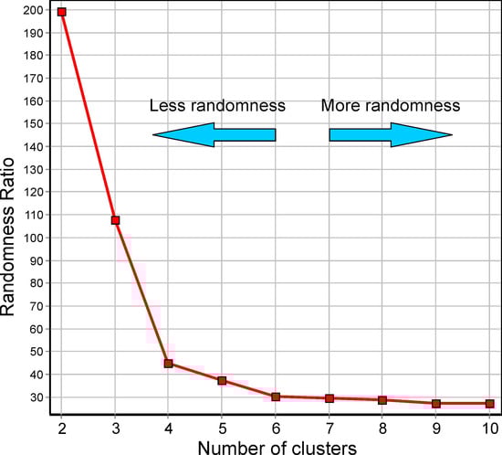
Figure 9.
Cluster randomness plot used for selecting a representative number of clusters (K) for the multivariate analysis of the wireline logging datasets recorded in the Cernavodă boreholes.
Figure 10 displays the multiborehole (joint datasets) clustering solutions obtained for K = 6 and K = 7, respectively. Table 3 presents depth estimates for the boundaries of the main geological complexes, derived from analyzing the continuity and similarity of clusters between the boreholes. Both the six-cluster and the seven-cluster solutions provided clear and detailed electrofacies typing and delineation, with a close match between the formation boundaries reported from drilling data and the boundaries estimated from clustering in the case of the BH-1 borehole (tracks 2 and 3 in Figure 10a—left and Figure 10b—left). The use of BH-1 as a depth calibration (reference) borehole to assess the accuracy of formation boundaries estimation through clustering allowed for the validation of the formation boundaries estimated for the BH-2 and BH-3 boreholes.
Table 4 presents the statistical parameters of the K = 6 and K = 7 clustering solutions obtained for the analyzed boreholes (cluster/electrofacies numbers are sorted in ascending order of the Iγ log response). Compared with the six-cluster solution (Figure 10a), the seven-cluster solution (Figure 10b) provided additional details within the main groundwater exploration target from the Cernavodă area—the Dolomite Complex. This complex is well defined by the predominance of electrofacies #4 and #5 (moderate Iγ, ρA, ϕN, and Δt mean values) in its upper part and of electrofacies #2 (lowest Iγ, ϕN, and Δt mean values; highest ρA mean values) in its lower part, corresponding to the cleanest and tightest carbonates on the intervals 550–697 m in BH-1, 556–698 m in BH-2, and 553–696 m in BH3.
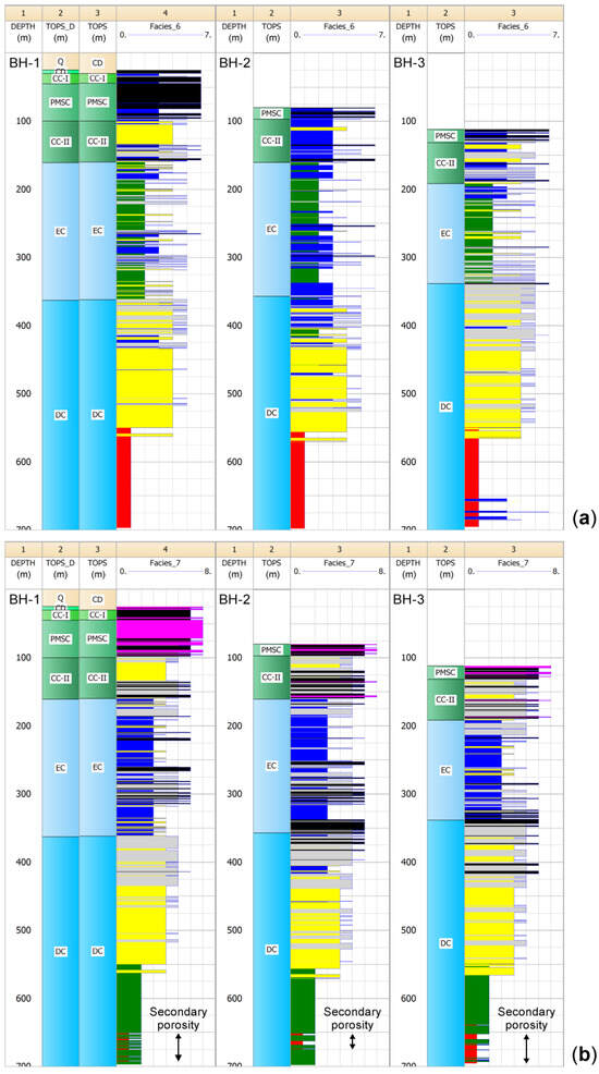
Figure 10.
Results of the K-means cluster analysis of the wireline logging datasets recorded in the Cernavodă boreholes: (a) clustering solution obtained for K = 6; (b) clustering solution obtained for K = 7. TOPS_D—formation boundaries reported from drilling data and geological analyses (m); TOPS—formation boundaries estimated from cluster analysis (electrofacies correlation) (m).
Table 3.
Estimation of the likely formation boundary depths for the Cernavodă boreholes, based on multiborehole cluster analysis results. The formation boundary depths reported from drilling data for the BH-1 borehole are provided for comparison.
Table 3.
Estimation of the likely formation boundary depths for the Cernavodă boreholes, based on multiborehole cluster analysis results. The formation boundary depths reported from drilling data for the BH-1 borehole are provided for comparison.
| Formation Boundaries | BH-1 | BH-2 | BH-3 | |
|---|---|---|---|---|
| Reported (m) | Estimated (m) | Estimated (m) | Estimated (m) | |
| Q/CD | 25.0 | |||
| CD/CC-I | 30.0 | 29.9 | ||
| CC-I/PMSC | 45.0 | 44.7 | ||
| PMSC/CC-II | 100.0 | 99.6 | 97.2 | 131.7 |
| CC-II/EC | 161.0 | 160.0 | 160.6 | 191.8 |
| EC/DC | 363.0 | 361.8 | 357.0 | 338.5 |
Q—Quaternary Continental Deposits, CD—Early Cretaceous Continental Deposits (Kap23), CC-I—Carbonate Complex I (Kbe3–va1), PMSC—Polychrome Marlstones and Shales Complex (Kbe12), CC-II—Carbonate Complex II (Kbe1), EC—Evaporite Complex (Jti3), DC—Dolomite Complex (Jki–ti12).
Table 4.
Statistical parameters (means and standard deviations—SD) of the K = 6 and K = 7 clustering solutions/electrofacies obtained for the Cernavodă boreholes.
Table 4.
Statistical parameters (means and standard deviations—SD) of the K = 6 and K = 7 clustering solutions/electrofacies obtained for the Cernavodă boreholes.
| Cluster # | Data Points | GR (cps) | SHN (Ω m) | LONG (Ω m) | NPHI (V/V) | DT (μs/ft) | |||||
|---|---|---|---|---|---|---|---|---|---|---|---|
| Mean | SD | Mean | SD | Mean | SD | Mean | SD | Mean | SD | ||
| K = 6 | |||||||||||
| 1 | 3977 | 7.959 | 3.694 | 707.457 | 1.622 | 1793.081 | 1.701 | 0.096 | 0.041 | 63.758 | 21.840 |
| 2 | 3239 | 17.792 | 6.026 | 151.015 | 1.632 | 361.160 | 1.924 | 0.460 | 0.061 | 66.733 | 9.427 |
| 3 | 3021 | 25.454 | 6.815 | 45.678 | 1.545 | 82.016 | 1.642 | 0.314 | 0.078 | 96.805 | 23.330 |
| 4 | 4725 | 25.910 | 5.302 | 104.988 | 1.360 | 223.512 | 1.454 | 0.231 | 0.063 | 67.865 | 8.368 |
| 5 | 2737 | 37.711 | 6.969 | 62.463 | 1.463 | 133.321 | 1.620 | 0.324 | 0.072 | 81.458 | 13.720 |
| 6 | 923 | 42.434 | 7.981 | 25.601 | 1.573 | 38.300 | 1.716 | 0.439 | 0.095 | 165.867 | 27.420 |
| K = 7 | |||||||||||
| 1 | 520 | 5.785 | 1.765 | 394.912 | 1.746 | 835.853 | 1.748 | 0.169 | 0.060 | 128.789 | 31.360 |
| 2 | 3556 | 8.143 | 3.733 | 741.669 | 1.595 | 1921.366 | 1.643 | 0.090 | 0.038 | 57.645 | 10.220 |
| 3 | 3310 | 17.938 | 6.352 | 149.324 | 1.644 | 356.312 | 1.947 | 0.460 | 0.061 | 67.225 | 9.995 |
| 4 | 3978 | 25.958 | 5.770 | 113.177 | 1.326 | 244.974 | 1.412 | 0.220 | 0.061 | 66.978 | 7.980 |
| 5 | 4706 | 29.838 | 7.133 | 57.328 | 1.387 | 112.954 | 1.501 | 0.302 | 0.059 | 77.936 | 10.090 |
| 6 | 1954 | 35.846 | 9.696 | 41.824 | 1.621 | 76.507 | 1.821 | 0.355 | 0.086 | 113.833 | 16.050 |
| 7 | 598 | 43.351 | 7.583 | 22.046 | 1.443 | 31.501 | 1.622 | 0.473 | 0.085 | 181.870 | 18.640 |
Within these tight sections of the boreholes, electrofacies #1 from the seven-cluster solution (lowest Iγ, moderate ρA and ϕN, and highest Δt mean values) can be related to zones with a significant secondary porosity development and water-producing potential. Based on the extent of electrofacies #1 (red color in Figure 10b), these zones appear in the intervals 651–693 m in BH-1, 652–675 m in BH-2, and 639–696 m in BH-3.
Considering the 8.5 in. final sections of the boreholes, the highest occurrence of electrofacies #1 was observed in BH-3 (320 data levels), compared to BH-1 (108 data levels) and BH-2 (92 data levels). Such zones were not detected by the caliper tool run in the BH-2 borehole (CAL curve from Figure 5), possibly because isolated karst cavities were not intersected by the tool’s arms.
Figure 11 shows multiborehole crossplots of the wireline logs jointly used in the cluster analysis, together with histograms of these logs, with data included from all the boreholes. The crossplots help visualize the particular log response combinations that defined the obtained seven-cluster solution. The correspondence between the main geological complexes/lithofacies and the principal cluster/electrofacies combinations is as follows: Quaternary and Early Cretaceous Continental Deposits—#7 (predominant) and #6 (subordinate); Carbonate Complex I—#6 (predominant) and #7 (subordinate); Polychrome Marlstones and Shales Complex—#7 (predominant) and #6 (subordinate); Carbonate Complex II—#4 (predominant) and #5 (subordinate); Evaporite Complex—#3 (predominant) and #5 (subordinate); Dolomite Complex (upper section)—#4 (predominant) and #5 (subordinate); and Dolomite Complex (lower section)—#2 (predominant) and #1 (subordinate).
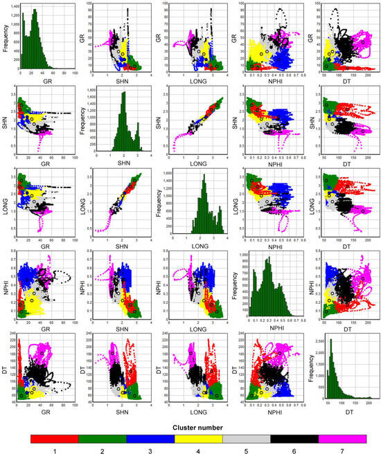
Figure 11.
Illustration of the clustering solution obtained for K = 7, by means of multiborehole crossplots of the wireline logs used in the cluster analysis (ρA input data in logarithmic form). The circles mark the location of the final centroid for each data cluster.
The Δt vs. ϕN (DT vs. NPHI) dependencies had a good resolution for overall formation delineation and lithological classification, whereas the Δt vs. ρA (DT vs. LONG and DT vs. SHN) and the Δt vs. Iγ (DT vs. GR) dependencies provided a better separation of electrofacies #1, which likely associated with the fractured or karstified water-bearing zones.
5.3. Quantitative Log Interpretation Results
The approach and results of the wireline logging data inversion are exemplified in Figure 12 for the BH-1 borehole, which had the largest log coverage depthwise, encompassing the entire J3–K1 carbonate suite from the Cernavodă area. The investigated interval was divided into six interpretation zones, according to the formation boundary depths identified from the drilling data and cluster analysis (track 2). The depth-constrained inversion was carried out separately for each zone, using distinct multimineral models with varying mixtures of quartz, calcite, dolomite, gypsum, anhydrite, clay, and water (effective porosity ϕ), in relation to the dominant lithology of the geological complexes. An additional advantage of the zonal inversion approach employed in this study is the possibility of using interpretation models with more volumetric components than the number of available input logs would allow. Track 3 from Figure 12 shows the final (optimal) interpretation model resulting from the combination of the zonal models and providing a comprehensive litho-porosity characterization of the interval. The quality of the inversion results can be evaluated through the normalized total fitting error (track 4—TotErr curve; fitting error values greater than 1.0 are highlighted in red) and also through the degree of fitting for the main input logs by the theoretical response of the models, i.e., by the corresponding reconstructed/synthetic logs (tracks 5–7; curves GR_r, NPHI_r, and DT_r are the reconstructed Iγ, ϕN, and Δt logs, representing the theoretical response of the optimal interpretation model). The uncertainties assigned to the main input logs are visualized via the error/confidence bands (yellow shading) delimited by the curves GR_pe, NPHI_pe, DT_pe (+σ) and GR_me, NPHI_me, DT_me (−σ).
To avoid a strong overestimation of ϕ from the sonic log on depth intervals with ϕS much larger than ϕN, we used a variable sonic uncertainty by setting a Δt threshold of 120 μs/ft. Thus, for measured Δt ≤ 120 μs/ft, we used σDT = 3 μs/ft as the default uncertainty, and for Δt > 120 μs/ft, we imposed a very large σDT, i.e., a very low (negligible) weighting factor for the sonic log contribution to the inversion solution. In Figure 12—track 7, this is reflected by the wide input confidence bands of the sonic log on the intervals with abnormally high Δt readings. The final interpretation models obtained for all the Cernavodă boreholes provided the best overall reconstruction of input logs. The larger data fitting errors are explainable by unfavorable measurement conditions, simplifications adopted for the model, or the local variability in the formation parameters (e.g., small-scale lithological/mineral heterogeneity or changes in the Archie parameters).
A correlation of the log interpretation models obtained for the analyzed boreholes is presented in Figure 13, together with a reconstruction of the measured ρA,64 logs (LONG curves) by means of theoretical ρo logs (Ro curves) corresponding to Sw = 1. As observed, the Evaporite Complex, which overlies the Dolomite Complex exploration target, thins out in the SE–NW direction, from BH-1 towards BH-3. Within the Dolomite Complex, the dolomitization of pre-existing limestones (evaluated through the computed Vdolomite fractions) appears vertically uneven, occurring mostly in the upper part and, to some extent, the middle part of the complex and suggesting a downward circulation of the magnesium-rich fluids.
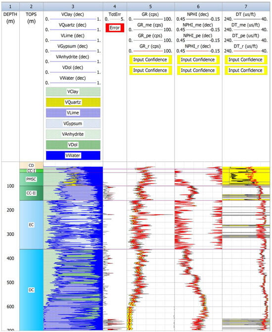
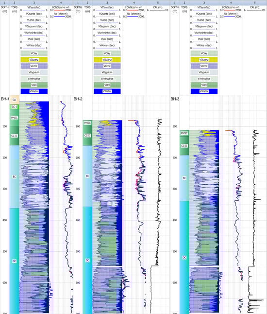
Figure 12.
Example of petrophysical interpretation results based on depth-constrained (zonal) inversion of the wireline logs recorded in the BH-1 borehole. The formation boundaries obtained from cluster analysis (TOPS track) define the depth intervals for each distinct multimineral model used.
Figure 13.
Optimal petrophysical interpretation models obtained from depth-constrained (zonal) inversion of the wireline logs recorded in the Cernavodă boreholes. The measured ρA,64 (LONG) and reconstructed ρo (Ro) resistivity logs are shown in tracks 4 (Ω m). For the BH-2 and BH-3 boreholes, the measured caliper (CAL) logs are presented in tracks 5 (in) to illustrate borehole size changes.
In agreement with the cluster analysis results (electrofacies #1 from the seven-cluster solution), the secondary porosity—indicated by significant and local increases in the computed effective porosity—appears to be preferentially developed in the lower part of the Dolomite Complex, within limestones less affected or not affected by dolomitization. In this regard, for the 8.5 in. sections of the analyzed boreholes (approximately 550–700 m depth) the computed maximum effective porosities are 0.277 for BH-1, 0.258 for BH-2, and 0.378 for BH-3, compared with computed mean effective porosities of 0.087 for BH-1, 0.071 for BH-2, and 0.088 for BH-3. The porosity due to fractures or fissures usually adds less than 0.01–0.02 and rarely adds up to 0.05 to the primary/matrix porosity [1], so it can be assumed that the higher ϕ values that resulted from the interpretation are related to vuggy porosity (e.g., karstic dissolution vugs or caverns). The association of the secondary porosity predominantly with nondolomitized limestones may result from the generally higher solubility of limestones compared to dolomites but also from an obliteration of pre-existing porosity via the dolomitization process [8,9] in the upper-middle parts of the Dolomite Complex.
Besides the vertical variability of the dolomitization, the log interpretation results also reveal a lateral (horizontal) heterogeneity in the Dolomite Complex. The dolomitization magnitude gradually increases from BH-1 to BH-3 (SE to NW). The mean Vdolomite fractions computed for the entire Dolomite Complex intervals are 0.288 for BH-1, 0.357 for BH-2, and 0.363 for BH-3. For the 8.5 in. borehole sections within the complex, the mean Vdolomite fractions are 0.275 for BH-1, 0.318 for BH-2, and 0.356 for BH-3. This progressive lateral increase may indicate a tectonic–structural control of the flow pathways for the dolomitizing fluids that is related to a variable degree of fracturing and, consequently, the pore space connectivity and permeability in the Dolomite Complex—highest for BH-3, lowest for BH-1 boreholes. Consequently, the SE to NW direction could correspond to a trend of increasing groundwater productivity, which represents an important practical outcome of this study for the drilling of future exploitation boreholes in the Cernavodă area and in neighboring sectors.
The best overall reconstruction of the recorded long normal ρA,64 logs through synthetic ρo logs was achieved for ρw values of 15–20 Ω m (Figure 13—tracks 4). Downhole temperature data were available for the 8.5 in. final sections of BH-2 and BH-3 boreholes, and the measured T ranged from 20.4 to 21.7 °C. Considering a mean T of 21 °C, the best-fit ρw range obtained corresponds to a groundwater mineralization (salinity) of 250–340 ppm NaCl equivalent [36], and the actual one depends on the specific ionic composition of the groundwater. The low mineralization obtained from log interpretation allowed for the characterization of the groundwater of Cernavodă carbonate reservoirs as fresh.
5.4. Groundwater Production Analysis (Borehole Testing)
After completion, the boreholes were tested for groundwater production from the 8.5 in. sections that penetrated the lower part of the Late Jurassic Dolomite Complex. The boreholes were equipped with submersible pumps installed at a 32 m depth, and constant rate discharge tests were performed through pumping (Figure 14). The results are presented in Table 5.
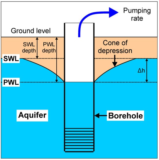
Table 5.
Results of the groundwater pumping tests performed for the Cernavodă boreholes.
Table 5.
Results of the groundwater pumping tests performed for the Cernavodă boreholes.
| Borehole | SWL (m) | PWL (m) | Q (L/s) | SC (L/s/m) |
|---|---|---|---|---|
| BH-1 | 4.00 | 10.00 | 16.0 | 2.67 |
| BH-2 | 3.10 | 5.00 | 28.5 | 15.00 |
| BH-3 | 5.17 | 5.92 | 21.2 | 28.27 |
SWL—static water level, PWL–pumping (dynamic) water level, Q—discharge (pumping rate), SC—specific capacity.
Figure 14.
Illustration of a pumping test performed for a groundwater exploitation borehole. SWL—static water level (m), PWL—pumping water level (m), Δh—drawdown (m).
To evaluate the test results, we calculated the specific capacity in Table 5 as SC = Q/Δh, where Δh = PWL − SWL is the drawdown (m) in a borehole resulting from the aquifer’s response to pumping. Generally, the SC is an important indicator of borehole productivity and reflects, to a certain extent, the aquifer’s quality (e.g., porosity, permeability). Higher SC values indicate more productive boreholes, yielding more groundwater for a given drawdown.
The SC comparison indicates important differences between the boreholes: BH-1 has the lowest productivity, BH-3 has the highest productivity, and BH-2 has an intermediate productivity. The pumping test results are partially supported by the petrophysical interpretation models, which showed a significantly higher maximum porosity at the base of the Dolomite Complex in the BH-3 borehole compared with BH-1 and BH-2. However, the large disparity in productivity between the BH-1 and BH-2 boreholes, which are in close proximity to each other, cannot be explained based on their comparable maximum and mean porosities computed for their final sections. In this case, the main controlling factors for the observed differences in groundwater productivity are likely the variable degree of pore space connectivity and fracture permeability of the carbonate-rock aquifer. This interpretation is in agreement with the increased extent of dolomitization indicated by the log interpretation from BH1 towards BH3, which suggests an increased fracture density and better flow characteristics in the SE to NW direction. Such an outcome of the present study could significantly improve the placement of additional boreholes for a more efficient exploitation of the aquifer.
The analyses conducted on groundwater samples collected from the BH-1 and BH-2 boreholes showed electrical conductivities in the 714–721 μS/cm range (equivalent to ρw ≈ 14 Ω m), total dissolved solids concentrations of 533–539 mg/L, and an average salinity of 0.3 g/L (300 ppm). The ρw and salinity measured on the samples match the values obtained from logging data inversion, validating the interpretation methodology and the parameter selection.
6. Conclusions
This study aimed to evaluate the petrophysical and reservoir properties of the most important aquifer system in southern–southeastern Romania, the Late Jurassic–Early Cretaceous (J3–K1) groundwater body shared with Bulgaria and developed in karstic–fractured carbonates. We analyzed three 700 m deep groundwater exploration–exploitation boreholes drilled in the Cernavodă town area, South Dobrogea region, Romania, which intercepted in their lower sections the J3-age Rasova Formation (the water-bearing “Dolomite Complex”), where significant secondary porosity is present in carbonate deposits ranging from limestones to dolomites. Our investigation utilized an approach combining geophysical wireline logging, drilling and geological data, multiborehole cluster analysis, and zonal inversion of the logging data with variable confidence assigned to the input logs, as well as groundwater pumping tests, sampling, and analysis. The following conclusions can be drawn from this research:
- In the studied area, and likely in the entire Cernavodă tectonic block, the main interval with secondary porosity development (karstic dissolution features, fractures) and the maximum water-producing potential is located in the lower part of the Rasova Formation (639–700 m depth), in the limestones least affected by dolomitization. This finding has an important practical implication for the planning and drilling program of subsequent groundwater exploitation boreholes;
- The pumping tests and log interpretation results demonstrate a strong heterogeneity of the aquifer, with highly variable borehole productivities even on short distances. This variability is not only due to differences in porosity but also to different degrees of hydraulic connectivity within the carbonate reservoir, which are likely related to tectonic factors (amount of fracturing) or unequal karst development;
- The SE to NW direction appears to correspond to a trend of increasing groundwater productivity in the Cernavodă area and, possibly, at a larger scale. This is also suggested by a direct correlation between productivity and the lateral (horizontal) intensity of the calcite-to-dolomite replacement, with the dolomitization extent reflecting pore space connectivity. If confirmed by further research, this novel outcome can help optimize the placement of future extraction boreholes.
The limitations of the present study are related to the relatively restricted geophysical investigation program conducted in the analyzed boreholes and the unfocused resistivity logging tool employed, which did not provide a minimization of the borehole conductive effect. However, within the main exploration target (the Rasova Formation), in the 8.5 in. final sections, the borehole effect upon the measured apparent resistivity data and the log interpretation results is minimal. A beneficial addition to the logging programs run in such carbonate reservoirs would be the inclusion of electrical, acoustic, and/or optical imaging tools for superior and highly detailed secondary porosity quantification and reservoir characterization.
Author Contributions
Conceptualization, B.M.N.; methodology, B.M.N. and M.M.B.; software, B.M.N., M.M.B. and A.T.; validation, B.M.N., M.M.B. and A.T.; formal analysis, B.M.N., M.M.B. and A.T.; investigation, B.M.N., M.M.B. and A.T.; resources, B.M.N.; data curation, B.M.N., M.M.B. and A.T.; writing—original draft preparation, B.M.N.; writing—review and editing, B.M.N., M.M.B. and A.T.; visualization, B.M.N., M.M.B. and A.T.; supervision, B.M.N.; project administration, B.M.N. and M.M.B. All authors have read and agreed to the published version of the manuscript.
Funding
This study was funded in the framework of the annual research plan of the Faculty of Geology and Geophysics—University of Bucharest.
Data Availability Statement
The data are available on request from the authors.
Acknowledgments
We would like to thank the two anonymous reviewers for their useful comments and suggestions that significantly improved the manuscript.
Conflicts of Interest
The authors declare no conflicts of interest.
Appendix A
MATLAB code for limestone neutron porosity (ϕN) computation based on the long-spacing and short-spacing detectors count rates:
where: Logs is a MATLAB (.mat) data file containing the vectors DEPTH (m), CAL—caliper values (inch), FAR—long-spacing detector count rates (cps), and NEAR—short-spacing detector count rates (cps); P is a vector storing the computed ϕN values (%); and N is the number of logging data samples in each vector. For the BH-1 borehole, the CAL curve (not available) was replaced with the bit size values.
| clear all; close all; clc load Logs; N = length(DEPTH); for i = 1:N CAL(i) = CAL(i) * 25.4; if NEAR(i) > 1 TMP1 = FAR(i)/NEAR(i); else TMP1 = 1; end TMP2 = TMP1 * TMP1; TMP3 = TMP2 * TMP1; P214 = 0.01080258/TMP3 − 0.2344151/TMP2 + 4.779079/TMP1 − 9.517288; P150 = 0.01149102/TMP3 − 0.2548200/TMP2 + 4.857260/TMP1 − 8.734154; if CAL(i) >= 214 P(i,1) = P214; elseif CAL(i) <= 150 P(i,1) = P150; else TMP4 = (P214 − P150)/64; TMP5 = P150 − TMP4 * 150; P(i,1) = TMP4 * CAL(i) + TMP5; end end dlmwrite(‘NPHI.txt’, [DEPTH P], ‘delimiter’, ‘\t’) |
References
- Tiab, D.; Donaldson, E.C. Petrophysics: Theory and Practice of Measuring Reservoir Rock and Fluid Transport Properties, 4th ed.; Gulf Professional Publishing: Houston, TX, USA, 2015; ISBN 978-0-12-803188-9. [Google Scholar]
- Asquith, G.B. Handbook of Log Evaluation Techniques for Carbonate Reservoirs; American Association of Petroleum Geologists: Tulsa, OK, USA, 1985; ISBN 0-89181-655-0. [Google Scholar]
- Ellis, D.W.; Singer, J.M. Well Logging for Earth Scientists, 2nd ed.; Springer: Dordrecht, The Netherlands, 2008; ISBN 978-1-4020-3738-2. [Google Scholar]
- Lucia, J.F. Carbonate Reservoir Characterization: An Integrated Approach, 2nd ed.; Springer: Berlin, Germany, 2007; ISBN 978-3-540-72740-8. [Google Scholar]
- Ahr, W.M. Geology of Carbonate Reservoirs: The Identification, Description, and Characterization of Hydrocarbon Reservoirs in Carbonate Rocks; John Wiley & Sons Inc.: Hoboken, NJ, USA, 2008; ISBN 978-0-470-16491-4. [Google Scholar]
- Schlumberger, Ltd. Log Interpretation Principles/Applications, 4th ed.; Schlumberger Educational Services: Houston, TX, USA, 1996. [Google Scholar]
- Asquith, G.; Krygowski, D. Basic Well Log Analysis, 2nd ed.; AAPG Methods in Exploration, No. 16; American Association of Petroleum Geologists: Tulsa, OK, USA, 2004; ISBN 0-89181-667-4. [Google Scholar]
- Machel, H.G. Concepts and models of dolomitization: A critical reappraisal. In Special Publications; Geological Society: London, UK, 2004; Volume 235, pp. 7–63. [Google Scholar] [CrossRef]
- Omidpour, A.; Mahboubi, A.; Moussavi-Harami, R.; Rahimpour-Bonab, H. Effects of dolomitization on porosity–permeability distribution in depositional sequences and its effects on reservoir quality, a case from Asmari Formation, SW Iran. J. Pet. Sci. Eng. 2022, 208, 109348. [Google Scholar] [CrossRef]
- Țenu, A.; Davidescu, F.; Petreș, R.; Coarnă, L. Environmental isotopes studies and the hydrogeological model of South Dobrogea (Romania). Theor. Appl. Karstology 2002, 15, 61–72. [Google Scholar]
- International Comission for the Protection of the Danube River (Danube River Basin Management Plan—Update 2021, Annex 8). Available online: https://www.icpdr.org/sites/default/files/nodes/documents/drbmp_update_2021_final_annexes_1-21.pdf (accessed on 1 September 2023).
- IGRAC (International Groundwater Resources Assessment Centre). Transboundary Aquifers of the World [map], Edition 2021, Scale 1: 50 000 000; IGRAC: Delft, The Netherlands, 2021; Available online: https://www.un-igrac.org/ (accessed on 1 September 2023).
- Machkova, M. Hydrogeological Settings in Dobrudja Area and Groundwater Monitoring Networks in Transboundary Aquifers. In Overexploitation and Contamination of Shared Groundwater Resources (NATO Science for Peace and Security Series C: Environmental Security); Darnault, C.J.G., Ed.; Springer: Dordrecht, The Netherlands, 2008; pp. 83–102. ISBN 978-1-4020-6983-3. [Google Scholar]
- Pulido-Bosch, A.; López-Chicano, M.; Calaforra, J.M.; Cal Vache, M.L.; Machkova, M.; Dimitrov, D.; Velikov, B.; Pentchev, P. Groundwater problems in the karstic aquifers of the Dobrich region, northeastern Bulgaria. Hydrol. Sci. J. 2009, 44, 913–927. [Google Scholar] [CrossRef]
- Zamfirescu, F.; Moldoveanu, V.; Dinu, C.; Pitu, N.; Albu, M.; Danchiv, A.; Nash, H. Vulnerability to pollution of karst aquifer system in Southern Dobrogea. In Impact of Industrial Activities on Groundwater, Proceedings of the International Hydrogeological Symposium, Constanţa, Romania, 23–28 May 1994; Bucharest University Press: Bucharest, Romania, 1994; pp. 591–602. [Google Scholar]
- Țenu, A.; Noto, P.; Cortecci, G.; Nuti, S. Environmental isotopic study of the Barremian-Jurassic aquifer in South Dobrogca (Romania). J. Hydrol. 1975, 26, 185–198. [Google Scholar] [CrossRef]
- Țenu, A.; Davidescu, F.; Slăvescu, A. Recherches isotopiques sur les eaux des formations calcaires dans la Dobroudja Méridionale (Roumanie). In Isotopes Techniques in Water Resources Development, Proceedings of the International Atomic Energy Agency (IAEA) Symposium, Vienna, Austria, 30 March–3 April 1987; International Atomic Energy Agency: Vienna, Austria, 1987; pp. 439–453. [Google Scholar]
- Țenu, A.; Davidescu, F.; Petreș, R.; Stănescu, G. Variation des ressources souterraine du Dobrogea du Sud (Roumanie), effet conjugué des causes climatiques et anthropiques. In Regional Management of Water Resources, Proceedings of the International Association of Hydrological Sciences (IAHS) Sixth Scientific Assembly, Maastricht, The Netherlands, 18–27 July 2001; IAHS Press: Wallingford, UK, 2001; pp. 131–137. [Google Scholar]
- Bishop, C.M. Neural Networks for Pattern Recognition; Clarendon Press: Oxford, UK, 1995; ISBN 9780198538646. [Google Scholar]
- Rencher, A.C. Methods of Multivariate Analysis (Wiley Series in Probability and Statistics), 2nd ed.; John Wiley & Sons: New York, NY, USA, 2002; ISBN 0-471-41889-7. [Google Scholar]
- Timm, N.H. Applied Multivariate Analysis; Springer: New York, NY, USA, 2002; ISBN 0-387-95347-7. [Google Scholar]
- Härdle, W.; Simar, L. Applied Multivariate Statistical Analysis, 2nd ed.; Springer: Berlin, Germany, 2007; ISBN 978-3-540-72243-4. [Google Scholar]
- Serra, O.; Abbott, H.T. The contribution of logging data to sedimentology and stratigraphy. SPE J. 1982, 22, 117–131. [Google Scholar] [CrossRef]
- Serra, O. Well Logging and Reservoir Evaluation; Editions Technip: Paris, France, 2007; ISBN 978-2-7108-0881-7. [Google Scholar]
- Serra, O. Well Logging Handbook; Editions Technip: Paris, France, 2008; ISBN 978-2-7108-0912-8. [Google Scholar]
- Săndulescu, M. Geotectonica României [Geotectonics of Romania]; Editura Tehnică: București, România, 1984. (In Romanian) [Google Scholar]
- Juravle, D.T. Geologia României, Volumul I—Geologia Terenurilor Est-Carpatice (Platformele şi Orogenul Nord-Dobrogean) [Geology of Romania, Volume I—Geology of the East-Carpathian Terrains (Platforms and the North-Dobrogea Orogen)]; Editura Stef: Iași, România, 2009; ISBN 978-973-1809-55-7. (In Romanian) [Google Scholar]
- Ionesi, L. Geologia Unităților de Platformă și a Orogenului Nord-Dobrogean [The Geology of the Platform Units and of the North Dobrogean Orogen]; Editura Tehnică: București, România, 1994; ISBN 973-31-0531-7. (In Romanian) [Google Scholar]
- Niculescu, B.M.; Andrei, G. Application of electrical resistivity tomography for imaging seawater intrusion in a coastal aquifer. Acta Geophys. 2021, 69, 613–630. [Google Scholar] [CrossRef]
- Avram, E.; Drăgănescu, A.; Szass, L.; Neagu, T. Stratigraphy of the outcropping Cretaceous deposits in Southern Dobrogea (SE Romania). Mém. Inst. Géol. Géophys. 1988, 33, 5–43. [Google Scholar]
- Avram, E.; Costea, I.; Dragastan, O.; Muţiu, R.; Neagu, T.; Şindilar, V.; Vinogradov, C. Distribution of the Middle-Upper Jurassic and Cretaceous facies in the Romanian eastern part of the Moesian Platform. Rev. Roum. Géol. 1996, 39–40, 3–33. [Google Scholar]
- Neagu, T.; Dragastan, O. Stratigrafia depozitelor Neojurasice şi Eocretacice din Dobrogea de Sud [Stratigraphy of the Neo-Jurassic and Eo-Cretaceous Deposits from Southern Dobrogea]. Stud. Cerc. Geol. Geofiz. Geogr. Geologie 1984, 29, 80–87. (In Romanian) [Google Scholar]
- Dragastan, O. Upper Jurassic and Lower Cretaceous Formations and Facies in the Eastern area of the Moesian Platform (South Dobrogea included). Analele Univ. Din București Geol. 1985, 34, 77–85. [Google Scholar]
- Raymer, L.L.; Hunt, E.R.; Gardner, J.S. An improved sonic transit time-to-porosity transform. In Proceedings of the Society of Petrophysicists and Well Log Analysts (SPWLA) 21st Annual Logging Symposium, Lafayette, LA, USA, 8–11 July 1980; pp. 1–13. [Google Scholar]
- Raiga-Clemenceau, J.; Martin, J.P.; Nicoletis, S. The concept of acoustic formation factor for more accurate porosity determination from sonic transit time data. Log Anal. 1988, 29, 54–60. [Google Scholar]
- Schlumberger, Ltd. Log Interpretation Charts; Schlumberger: Houston, TX, USA, 2013; ISBN 978-1-937949-10-5. [Google Scholar]
- Doveton, J.H. Geologic Log Analysis Using Computer Methods (AAPG Computer Applications in Geology, No. 2); American Association of Petroleum Geologists: Tulsa, OK, USA, 1994; ISBN 0-89181-701-8. [Google Scholar]
- Senergy Software, Ltd. Interactive Petrophysics 4.2—User Manual; Senergy Software Ltd.: Banchory, Scotland, UK, 2013. [Google Scholar]
- Poupon, A.; Leveaux, J. Evaluation of water saturation in shaly formations. Log Anal. 1971, 12, 3–8. [Google Scholar]
- Archie, G.E. The Electrical Resistivity Log as an Aid in Determining Some Reservoir Characteristics. Trans. Am. Inst. Min. Metall. Pet. Eng. 1942, 146, 54–62. [Google Scholar] [CrossRef]
- Doveton, J.H. Log Analysis of Subsurface Geology: Concepts and Computer Methods; John Wiley & Sons Inc.: New York, NY, USA, 1986; ISBN 978-0471893684. [Google Scholar]
Disclaimer/Publisher’s Note: The statements, opinions and data contained in all publications are solely those of the individual author(s) and contributor(s) and not of MDPI and/or the editor(s). MDPI and/or the editor(s) disclaim responsibility for any injury to people or property resulting from any ideas, methods, instructions or products referred to in the content. |
© 2024 by the authors. Licensee MDPI, Basel, Switzerland. This article is an open access article distributed under the terms and conditions of the Creative Commons Attribution (CC BY) license (https://creativecommons.org/licenses/by/4.0/).