
NOx Emission Prediction for Heavy-Duty Diesel Vehicles Based on Improved GWO-BP Neural Network

Abstract
1. Introduction
2. NOx Emission Prediction Model
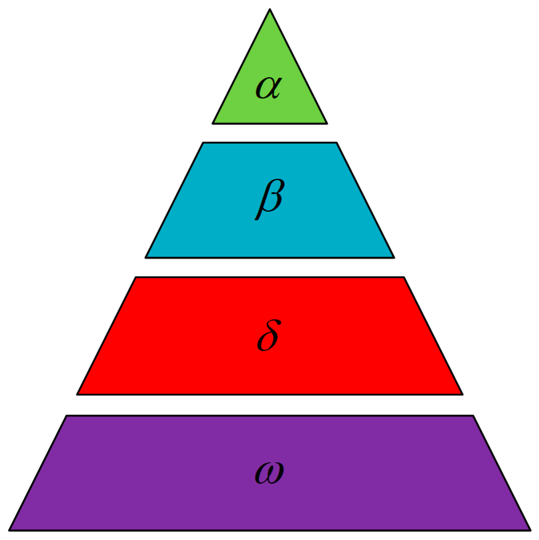
2.1. Gray Wolf Optimization Algorithm
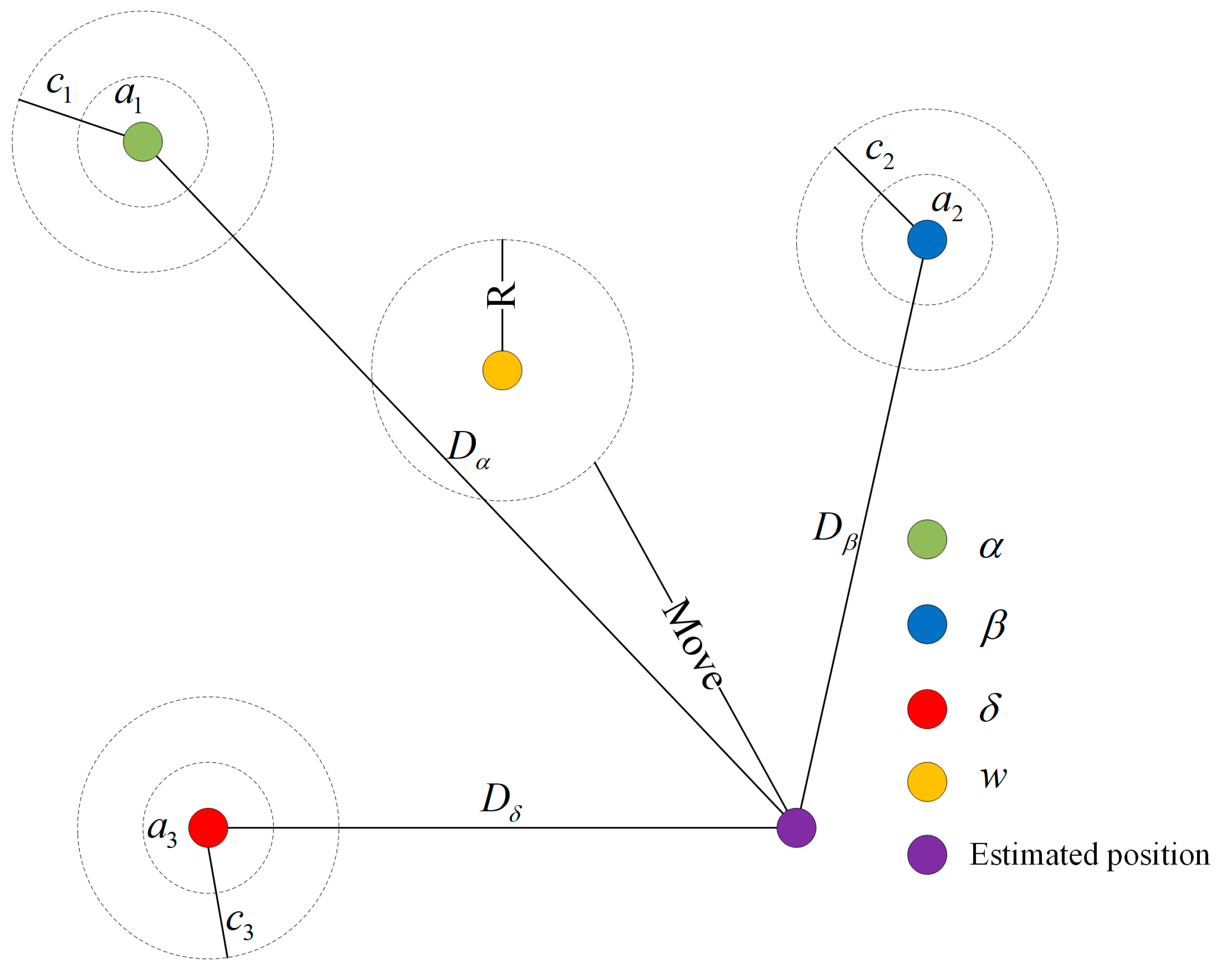
2.1.1. Surrounding Prey
2.1.2. Hunting
2.1.3. Attacking Prey
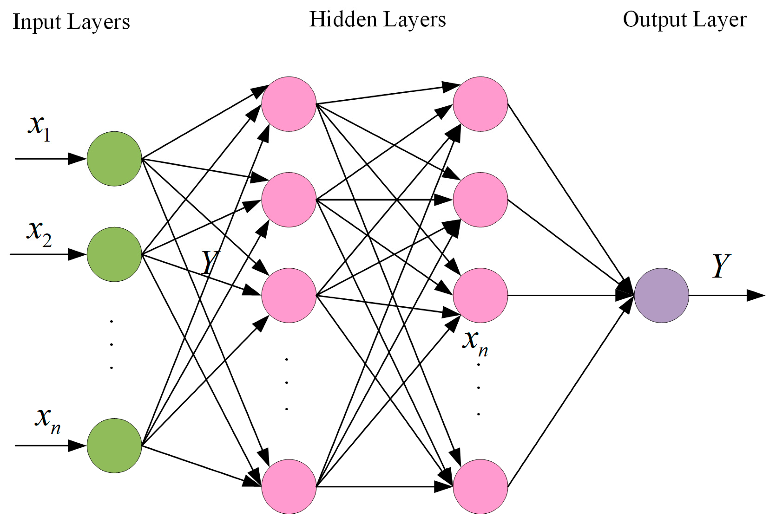
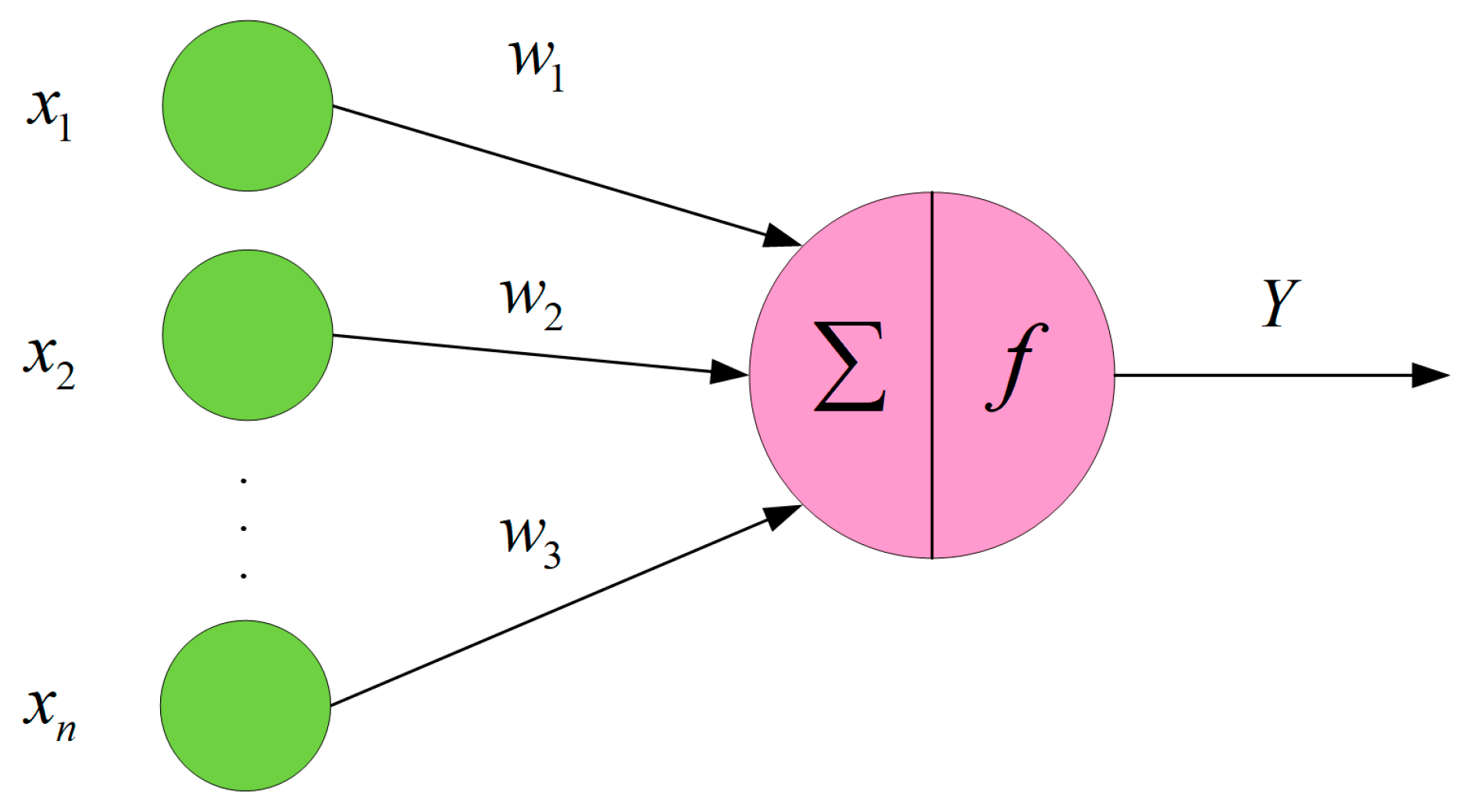
2.2. BP Neural Network
2.3. Improvement of Gray Wolf Optimization Neural Network
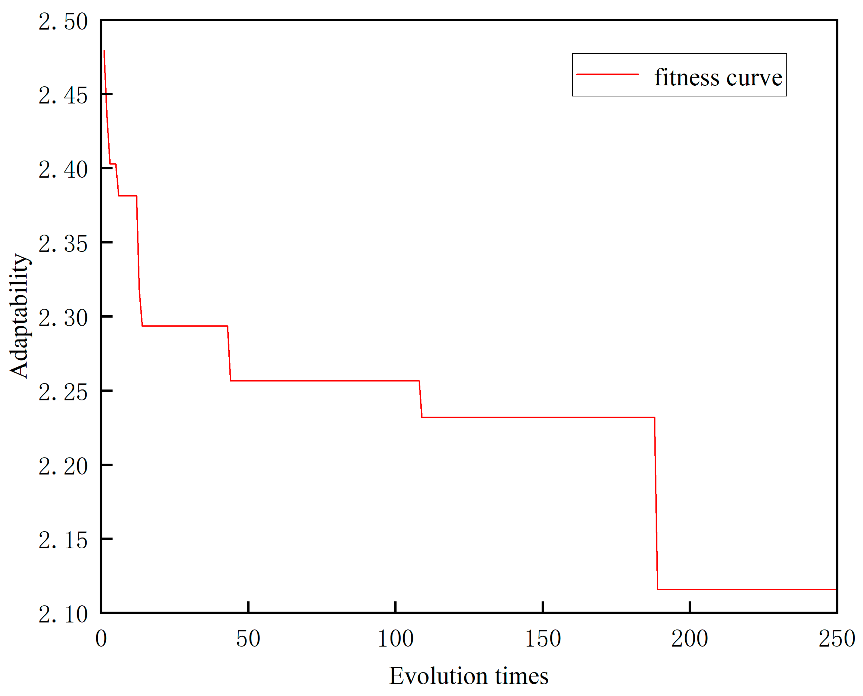
2.3.1. Gray Wolf Improvements
2.3.2. Gray Wolf Optimization BP Neural Network Model Building
3. Tests and Data Processing
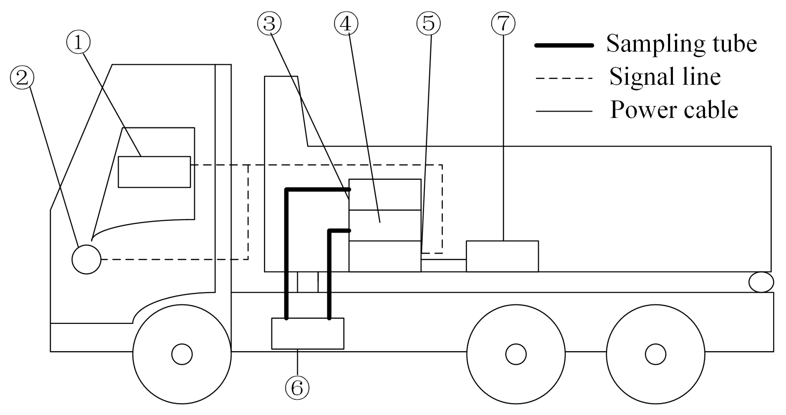
3.1. Test Equipment
3.2. Test Vehicles
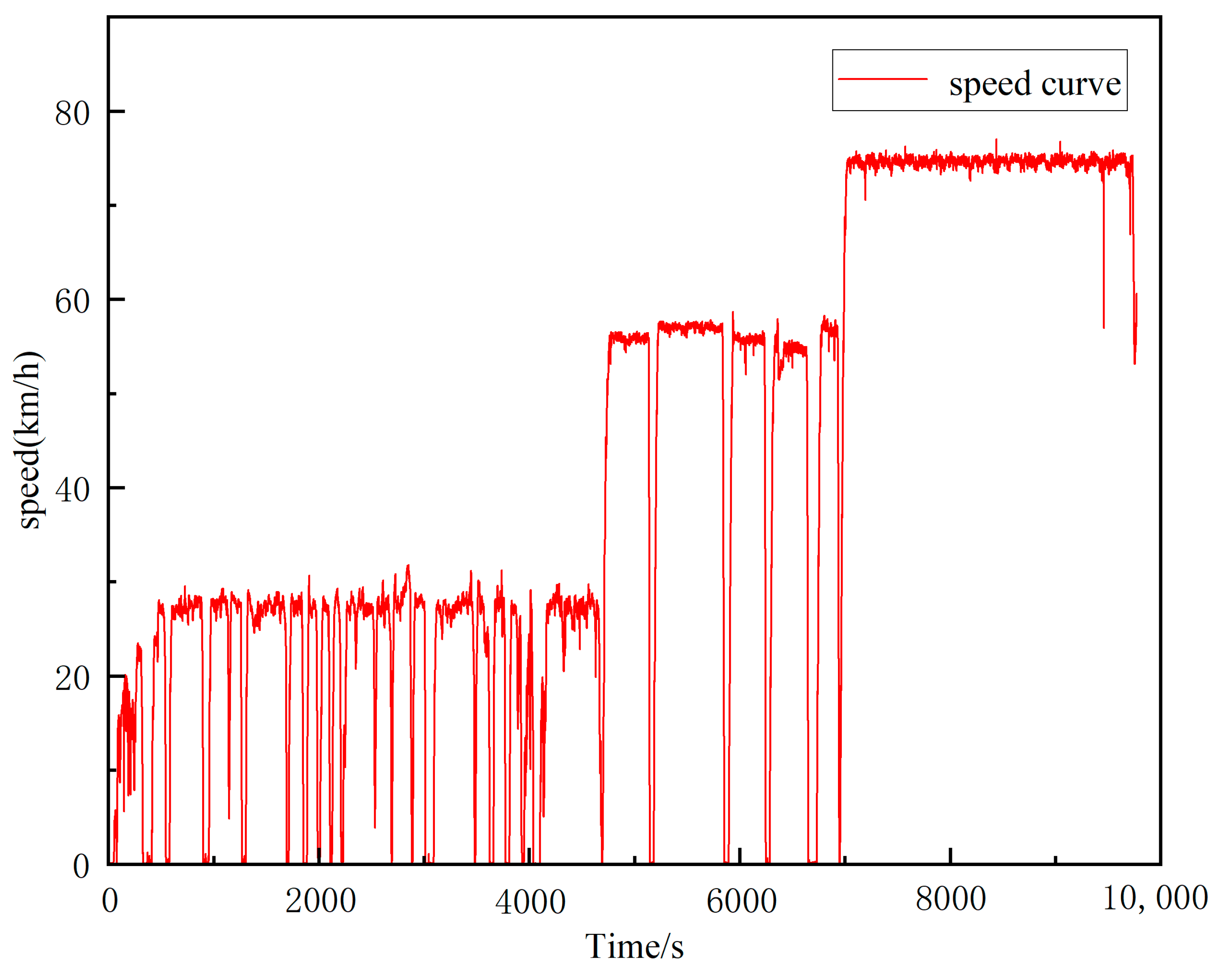
3.3. Road Tests
3.4. Data Pre-Processing
3.4.1. Invalid Data Culling
- Data during equipment inspection and zero drift verification.
- Data during cold engine start.
- Data that do not meet the test altitude and test ambient temperature requirements.
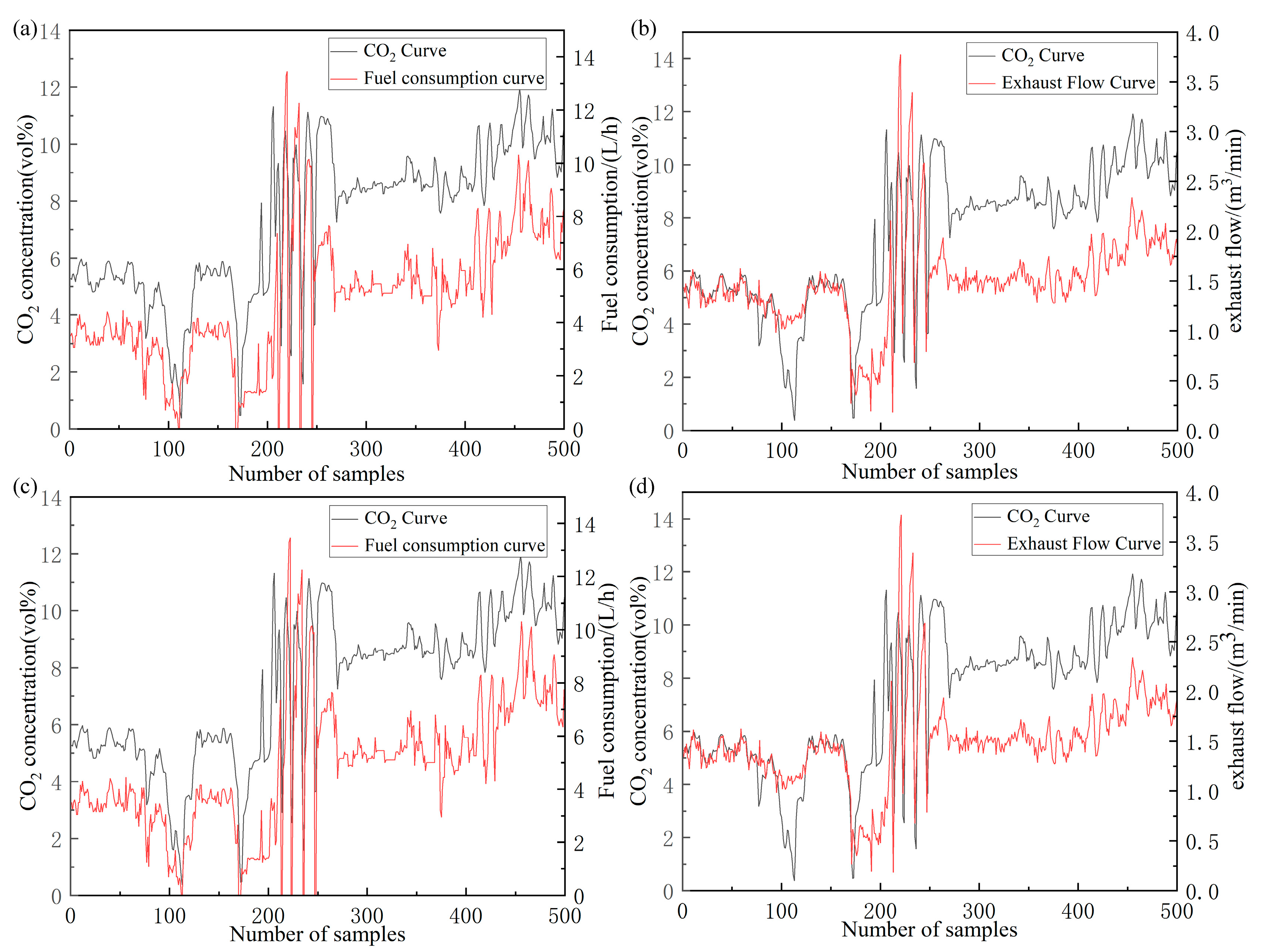
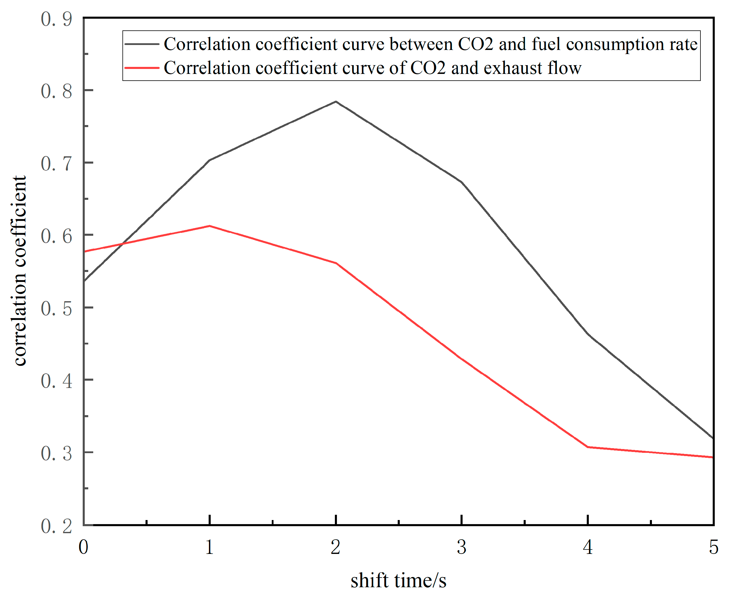
3.4.2. Data Alignment
- NOx, CO, and other data collected by the analyzer.
- Data such as exhaust gas mass flow rate and exhaust gas temperature collected by the exhaust gas flowmeter.
- Engine-related data collected by OBD.
3.4.3. Calculation of NOx Mass Emissions
3.4.4. Normalization of Data
3.5. Neural Network Parameterization
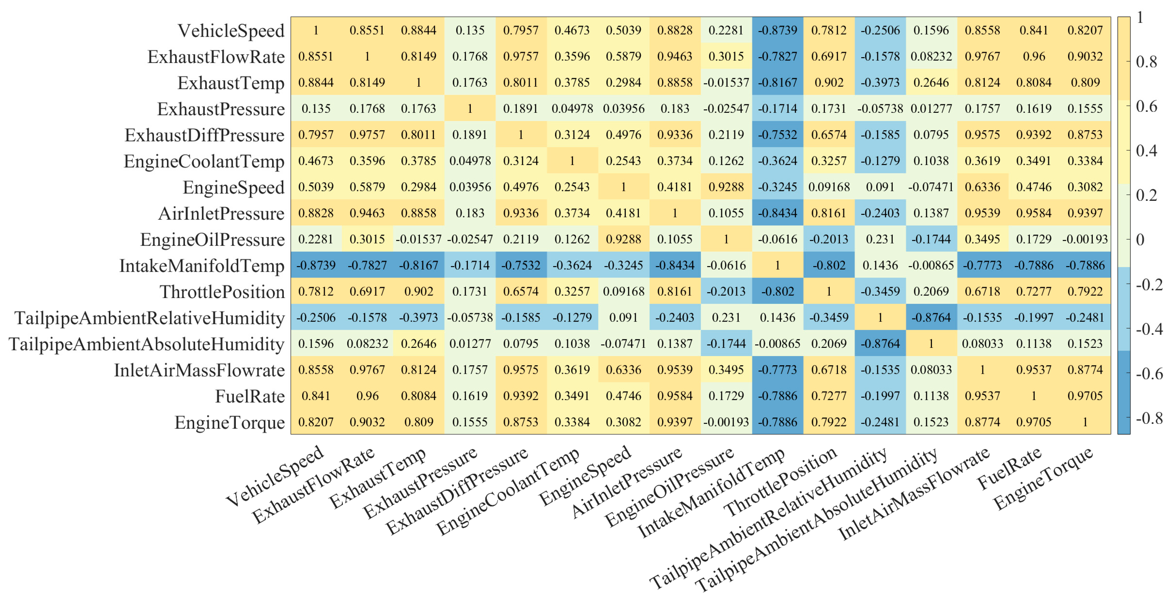
3.5.1. Input and Output Layer Determination
3.5.2. Determination of the Number of Hidden Layers and the Number of Neurons
3.5.3. Model Transfer Function Selection
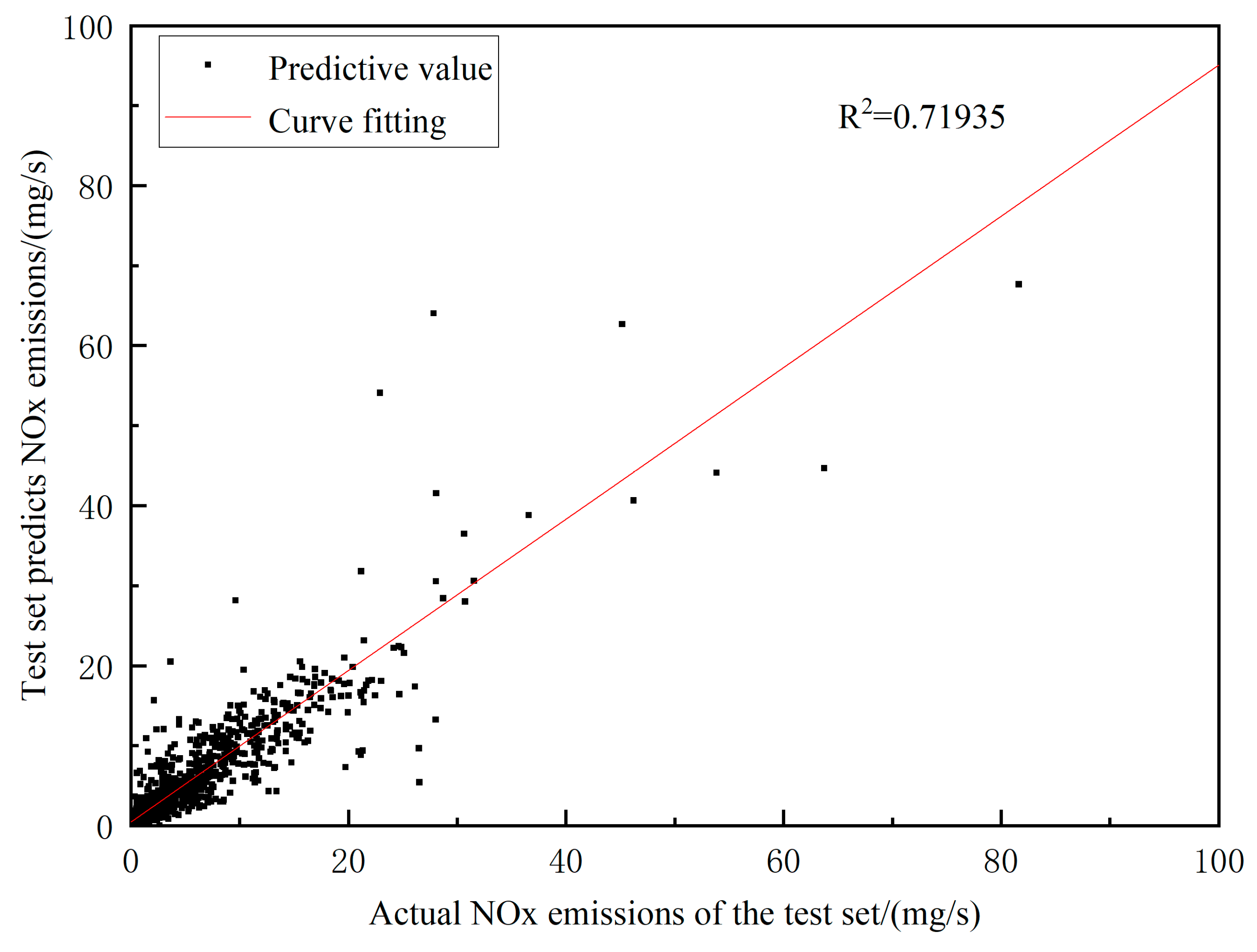
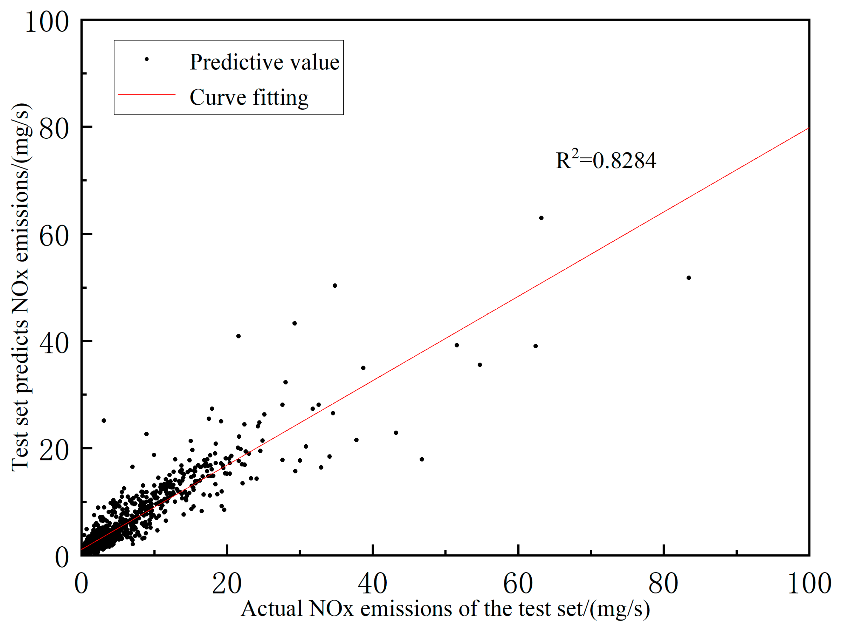
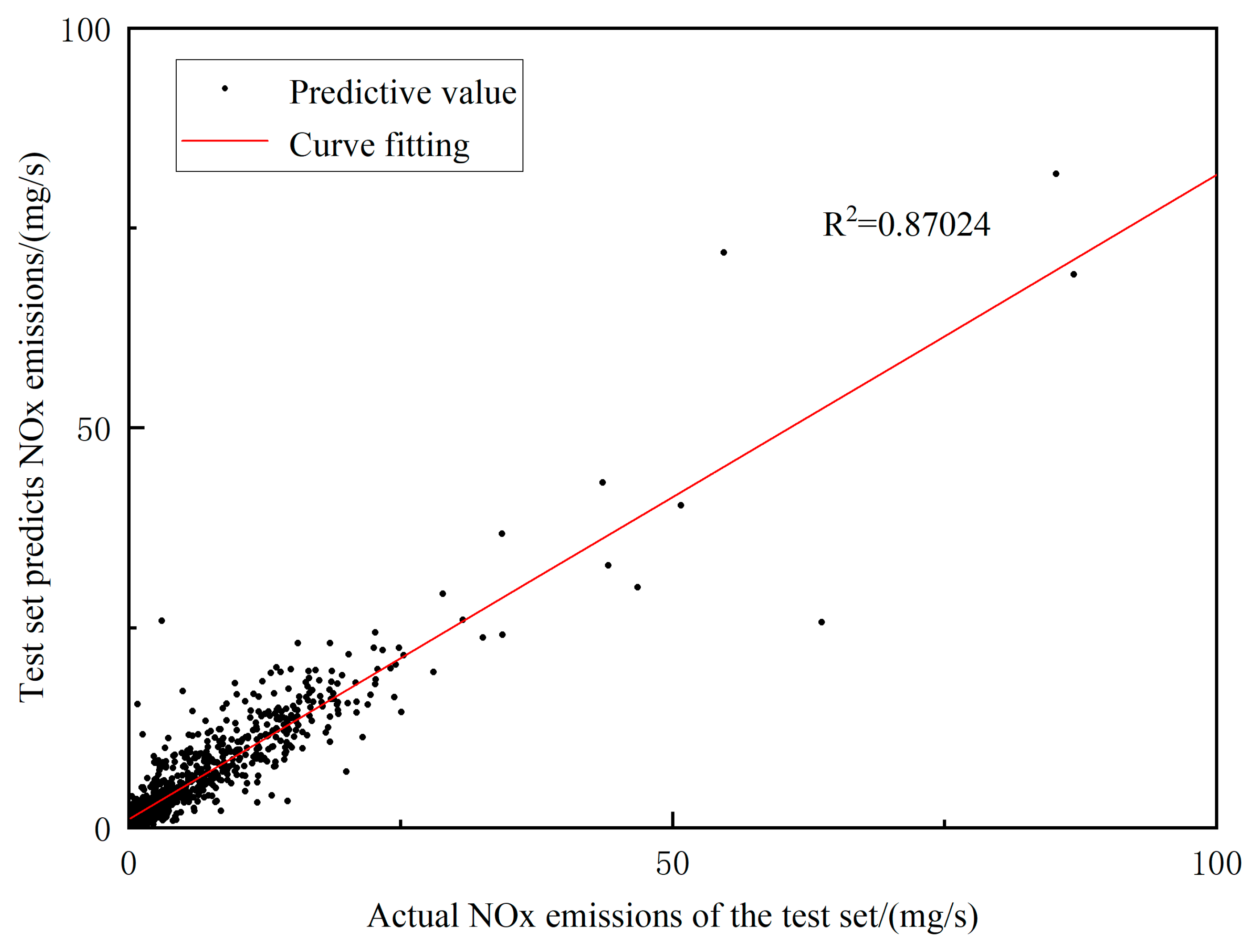
4. Analysis of Forecast Results
5. Conclusions
Author Contributions
Funding
Data Availability Statement
Acknowledgments
Conflicts of Interest
References
- Ministry of Ecology and Environment the People’s Republic of China. China Mobile Source Environmental Management Annual Report. 2021. Available online: http://www.gov.cn/xinwen/2021-09/11/content_5636764.htm (accessed on 5 January 2024).
- Wang, Y.; Hao, C.; Ge, Y. Fuel consumption and emission performance from light-duty conventional/hybrid-electric vehicles over different cycles and real driving tests. Fuel 2020, 278, 118340. [Google Scholar] [CrossRef]
- Guor, S.; Zhang, Y.; Cai, G.Q. Study on exhaust emission test of diesel vehicles based on PEMS. Procedia Comput. Sci. 2020, 166, 428–433. [Google Scholar] [CrossRef]
- Tang, G.; Wang, S.; Du, B.; Cui, L.; Huang, Y.; Xiao, W. Study on pollutant emission characteristics of different types of diesel vehicles during actual road cold start. Sci. Total Environ. 2022, 823, 153598. [Google Scholar] [CrossRef] [PubMed]
- Li, T.; Chen, X.; Yan, Z. Comparison of fine particles emissions of light-duty gasoline vehicles from chassis dynamometer tests and on-road measurements. Atmos. Environ. 2013, 68, 82–91. [Google Scholar] [CrossRef]
- Raparthi, N.; Debbarma, S.; Phuleria, H.C. Determination of heavy-duty vehicle emission factors from highway tunnel measurements in India: Laboratory vs. real-world study. Atmos. Pollut. Res. 2022, 13, 101581. [Google Scholar] [CrossRef]
- Liu, C.; Pei, Y.; Wu, C.; Zhang, F.; Qin, J. The impact of the variation in driving conditions on the NOx emissions characteristics in PEMS test for heavy-duty vehicle. J. Eng. Res. 2023. [Google Scholar] [CrossRef]
- Weiss, M.; Bonnel, P.; Kühlwein, J.; Provenza, A.; Lambrecht, U.; Alessandrini, S.; Carriero, M.; Colombo, R.; Forni, F.; Lanappe, G.; et al. Will Euro 6 reduce the NOx emissions of new diesel cars?–Insights from on-road tests with Portable Emissions Measurement Systems (PEMS). Atmos. Environ. 2012, 62, 657–665. [Google Scholar] [CrossRef]
- Tang, D.; Xu, Y.C.; Yao, S.D.; Li, C.Y.; Li, N. Prediction of emission performance in a diesel engine fuelled with bio-diesel based on double-hidden layer BP neural network. Appl. Mech. Mater. 2013, 278, 370–373. [Google Scholar]
- Fu, J.; Yang, R.; Li, X.; Sun, X.; Li, Y.; Liu, Z.; Zhang, Y.; Sunden, B. Application of artificial neural network to forecast engine performance and emissions of a spark ignition engine. Appl. Therm. Eng. 2022, 201, 117749. [Google Scholar] [CrossRef]
- Wang, G.; Awad, O.I.; Liu, S.; Shuai, S.; Wang, Z. NOx emissions prediction based on mutual information and back propagation neural network using correlation quantitative analysis. Energy 2020, 198, 117286. [Google Scholar] [CrossRef]
- Lee, J.; Kwon, S.; Kim, H.; Keel, J.; Yoon, T.; Lee, J. Machine learning applied to the NOx prediction of diesel vehicles under real driving cycle. Appl. Sci. 2021, 11, 3758. [Google Scholar] [CrossRef]
- Yu, H.; Chang, H.; Wen, Z.; Ge, Y.; Hao, L.; Wang, X.; Tan, J. Prediction of Real Driving Emission of Light Vehicles in China VI Based on GA-BP Algorithm. Atmosphere 2022, 13, 1800. [Google Scholar] [CrossRef]
- Natarajan, Y.; Wadhwa, G.; Sri Preethaa, K.R.; Paul, A. Forecasting Carbon Dioxide Emissions of Light-Duty Vehicles with Different Machine Learning Algorithms. Electronics 2023, 12, 2288. [Google Scholar] [CrossRef]
- Domínguez-Sáez, A.; Rattá, G.A.; Barrios, C.C. Prediction of exhaust emission in transient conditions of a diesel engine fueled with animal fat using Artificial Neural Network and Symbolic Regression. Energy 2018, 149, 675–683. [Google Scholar] [CrossRef]
- Çay, Y.; Korkmaz, I.; Çiçek, A.; Kara, F. Prediction of engine performance and exhaust emissions for gasoline and methanol using artificial neural network. Energy 2013, 50, 177–186. [Google Scholar] [CrossRef]
- Kim, S.; Kim, J. Assessing fuel economy and NOx emissions of a hydrogen engine bus using neural network algorithms for urban mass transit systems. Energy 2023, 275, 127517. [Google Scholar] [CrossRef]
- Ganesan, P.; Rajakarunakaran, S.; Thirugnanasambandam, M.; Devaraj, D. Artificial neural network model to predict the diesel electric generator performance and exhaust emissions. Energy 2015, 83, 115–124. [Google Scholar] [CrossRef]
- Mirjalili, S.; Mirjalili, S.M.; Lewis, A. Grey wolf optimizer. Adv. Eng. Softw. 2014, 69, 46–61. [Google Scholar] [CrossRef]
- Reeves, C.; Rowe, J.E. Genetic Algorithms: Principles and Perspectives: A Guide to GA Theory; Springer Science & Business Media: Berlin/Heidelberg, Germany, 2002; Volume 20. [Google Scholar]
- Marini, F.; Walczak, B. Particle swarm optimization (PSO). A Tutorial. Chemom. Intell. Lab. Syst. 2015, 149, 153–165. [Google Scholar] [CrossRef]
- Rojas, R. Neural Networks: A Systematic Introduction; Springer Science & Business Media: Berlin/Heidelberg, Germany, 2013. [Google Scholar]
- Rumelhart, D.E.; McClelland, J.L. Learning Internal Representations by Error Propagation. In Parallel Distributed Processing: Explorations in the Microstructure of Cognition: Foundations; MIT Press: Cambridge, MA, USA, 1987; pp. 318–362. [Google Scholar]
- Shah, B.; Trivedi, B. Optimizing back propagation parameters for anomaly detection. In Proceedings of the IEEE-International Conference on Research and Development Prospectus on Engineering and Technology (ICRDPET), Tamilnadu, South India, 29–30 March 2013. [Google Scholar]
- Hatta, N.M.; Zain, A.M.; Sallehuddin, R.; Shayfull, Z.; Yusoff, Y. Recent studies on optimization method of Grey Wolf Optimiser (GWO): A review (2014–2017). Artif. Intell. Rev. 2019, 52, 2651–2683. [Google Scholar] [CrossRef]
- Igiri, C.P.; Singh, Y.; Poonia, R.C. A review study of modified swarm intelligence: Particle swarm optimization, firefly, bat and gray wolf optimizer algorithms. Recent Adv. Comput. Sci. Commun. (Former. Recent Pat. Comput. Sci.) 2020, 13, 5–12. [Google Scholar] [CrossRef]
- Zhang, X.; Hou, J.; Wang, Z.; Jiang, Y. Joint SOH-SOC estimation model for lithium-ion batteries based on GWO-BP neural network. Energies 2022, 16, 132. [Google Scholar] [CrossRef]
- Xu, L.; Wang, H.; Lin, W.; Gulliver, T.A.; Le, K.N. GWO-BP neural network-based OP performance prediction for mobile multiuser communication networks. IEEE Access 2019, 7, 152690–152700. [Google Scholar] [CrossRef]
- Guo, Z.; Chen, L.; Gui, L.; Du, J.; Yin, K.; Do, H.M. Landslide displacement prediction based on variational mode decomposition and WA-GWO-BP model. Landslides 2020, 17, 567–583. [Google Scholar] [CrossRef]
- Tian, Y.; Yu, J.; Zhao, A. A predictive model of energy consumption for office building by using improved GWO-BP. Energy Rep. 2020, 6, 620–627. [Google Scholar] [CrossRef]
- Li, Z.; Liu, D.; Lu, F. Research on SOC estimation of lithium battery based on GWO-BP neural network. In Proceedings of the 2020 15th IEEE Conference on Industrial Electronics and Applications (ICIEA), Kristiansand, Norway, 9–13 November 2020; IEEE: New York, NY, USA, 2020; pp. 506–510. [Google Scholar]
- Ministry of Ecology and Environment the People’s Republic of China. Limits and Measurement Methods for Emissions from Diesel Fuelled Heavy-Duty Vehicles (CHINA VI). 2018. Available online: https://www.mee.gov.cn/ywgz/fgbz/bz/bzwb/dqhjbh/dqydywrwpfbz/201807/t20180703_445995.shtml (accessed on 5 January 2024).
- Gökhan, A.K.S.U.; Güzeller, C.O.; Eser, M.T. The effect of the normalization method used in different sample sizes on the success of the artificial neural network model. Int. J. Assess. Tools Educ. 2019, 6, 170–192. [Google Scholar]
- Bhanja, S.; Das, A. Impact of data normalization on deep neural network for time series forecasting. arXiv 2018, arXiv:1812.05519. [Google Scholar]
- Fang, R.; Shang, R.; Wu, M.; Peng, C.; Guo, X. Application of gray relational analysis to k-means clustering for dynamic equivalent modeling of the wind farm. Int. J. Hydrog. Energy 2017, 42, 20154–20163. [Google Scholar] [CrossRef]
- Maćkiewicz, A.; Ratajczak, W. Principal components analysis (PCA). Comput. Geosci. 1993, 19, 303–342. [Google Scholar] [CrossRef]


| Pollutants | Principle | Range | Zero Gas | Measuring Distance Gas | Measurement Distance Gas Pressure | Measurement Distance Gas Flow | Measurement Error |
|---|---|---|---|---|---|---|---|
| CO | NDIR | 10 vol% | Synthetic air | Gas mixture and | 100 kPa 10 kPa | 2.5~4.0 L/min | ppm |
| NDIR | 20 vol% | ||||||
| NOx | CLD | 1600 ppm |
| Parameters | Numerical Value |
|---|---|
| Vehicle Weight (kg) | 4390 |
| Maximum permissible gross mass (kg) | 8280 |
| Fuel type | 0# diesel |
| Maximum design speed (km/h) | 89 |
| Post-treatment system type | DOC + SCR + ASC + DPF |
| emission standard | Country VI |
| Vehicle type | N2 |
| Parameters | Digital | |||||
|---|---|---|---|---|---|---|
| NOx Emission (mg/s) | 17.62 | 19.19 | 5.81 | 2.16 | 0.54 | 4.08 |
| Vehicle Speed (km/h) | 27.57 | 27.96 | 27.18 | 56.43 | 55.83 | 74.75 |
| Exhaust Flow (m3/min) | 1.39 | 1.30 | 1.52 | 1.87 | 1.74 | 2.83 |
| Exhaust Temp (°C) | 78.57 | 86.25 | 130.07 | 180.12 | 166.97 | 200.12 |
| Exhaust Pressure (kPa) | 99.39 | 99.38 | 99.36 | 99.26 | 99.66 | 99.35 |
| Exhaust Diff Pressure (Pa) | 15.3 | 15.8 | 24.7 | 41.5 | 34.8 | 93.5 |
| Engine Coolant Temp (°C) | 83 | 85 | 84 | 84 | 85 | 85 |
| Engine speed (rpm) | 1677 | 1735.5 | 1618 | 1310.5 | 1284 | 1719.5 |
| Engine Torque (N·m) | 81.51 | 68.64 | 102.96 | 265.98 | 265.98 | 235.95 |
| Air Inlet Pressure (kPa) | 100 | 104 | 102 | 150 | 150 | 194 |
| Engine Oil Pressure (kPa) | 412 | 408 | 356 | 268 | 260 | 328 |
| Intake Manifold Temp (°C) | 44 | 43 | 48 | 44 | 43 | 44 |
| Throttle Position (%) | 19.6 | 19.6 | 19.6 | 90.8 | 90.8 | 90.8 |
| Tailpipe Ambient Relative Humidity (%) | 69.8 | 69.6 | 58.5 | 58.8 | 58.7 | 60.1 |
| Tailpipe Ambient Absolute Humidity (%) | 3.55 | 3.54 | 3.81 | 3.75 | 3.72 | 3.73 |
| Inlet Air Flowrate (kg/h) | 97.75 | 96 | 105 | 120.5 | 117.25 | 195.5 |
| Fuel Rate (L/h) | 3.3 | 2.95 | 3.5 | 7.95 | 8.05 | 8.9 |
Disclaimer/Publisher’s Note: The statements, opinions and data contained in all publications are solely those of the individual author(s) and contributor(s) and not of MDPI and/or the editor(s). MDPI and/or the editor(s) disclaim responsibility for any injury to people or property resulting from any ideas, methods, instructions or products referred to in the content. |
© 2024 by the authors. Licensee MDPI, Basel, Switzerland. This article is an open access article distributed under the terms and conditions of the Creative Commons Attribution (CC BY) license (https://creativecommons.org/licenses/by/4.0/).
Share and Cite
Wang, Z.; Feng, K. NOx Emission Prediction for Heavy-Duty Diesel Vehicles Based on Improved GWO-BP Neural Network. Energies 2024, 17, 336. https://doi.org/10.3390/en17020336
Wang Z, Feng K. NOx Emission Prediction for Heavy-Duty Diesel Vehicles Based on Improved GWO-BP Neural Network. Energies. 2024; 17(2):336. https://doi.org/10.3390/en17020336
Chicago/Turabian StyleWang, Zhihong, and Kai Feng. 2024. "NOx Emission Prediction for Heavy-Duty Diesel Vehicles Based on Improved GWO-BP Neural Network" Energies 17, no. 2: 336. https://doi.org/10.3390/en17020336
APA StyleWang, Z., & Feng, K. (2024). NOx Emission Prediction for Heavy-Duty Diesel Vehicles Based on Improved GWO-BP Neural Network. Energies, 17(2), 336. https://doi.org/10.3390/en17020336