Abstract
Sub-hourly load forecasting can provide accurate short-term load forecasts, which is important for ensuring a secure operation and minimizing operating costs. Decomposition algorithms are suitable for extracting sub-series and improving forecasts in the context of short-term load forecasting. However, some existing algorithms like singular spectrum analysis (SSA) struggle to decompose high sampling frequencies and rapidly changing sub-hourly load series due to inherent flaws. Considering this, we propose an empirical mode decomposition-based hybrid model, named EMDHM. The decomposition part of this novel model first detrends the linear and periodic components from the original series. The remaining detrended long-range correlation series is simplified using empirical mode decomposition (EMD), generating intrinsic mode functions (IMFs). Fluctuation analysis is employed to identify high-frequency information, which divide IMFs into two types of long-range series. In the forecasting part, linear and periodic components are predicted by linear and trigonometric functions, while two long-range components are fitted by long short-term memory (LSTM) for prediction. Four forecasting series are ensembled to find the final result of EMDHM. In experiments, the model’s framework we propose is highly suitable for handling sub-hourly load datasets. The MAE, RMSE, MARNE, and R2 of EMDHM have improved by 20.1%, 26.8%, 22.1%, and 5.4% compared to single LSTM, respectively. Furthermore, EMDHM can handle both short- and long-sequence, sub-hourly load forecasting tasks. Its R2 only decreases by 4.7% when the prediction length varies from 48 to 720, which is significantly lower than other models.
1. Introduction
Load forecasting holds immense significance within many fields, like the electric industry [1]. Numerous nations have privatized and deregulated their power systems, transforming electricity into a commodity traded at market prices. As load forecasts play a pivotal role in determining these prices, they have become indispensable for the supply industry [2]. Short-term load forecasting (STLF), in particular, is necessary for reliable timely and economic information to operate an energy system, and it is in the range of a few minutes to seven days [3]. For grids and power companies, the information gained through STLF not only aids in the optimal allocation of power generation capacity but also enables cost-effective unit scheduling within safe operational boundaries. A mere 1% reduction in the average prediction error can translate into potentially amounting to hundreds of thousands or even millions of dollars [4]. With a continuous commitment to optimizing electricity distribution, organizations such as independent system operators plan the allocation of available system resources to meet the hourly system load and ensure system security while minimizing operating costs [5]. What is more, the increasing deployment of advanced metering infrastructure has made hourly energy consumption data widely available [6]. Thus, forecasts with a finer time granularity are needed and are then better suited to assist in planning resource allocation in real time. Consequently, the research focus of STLF has shifted gradually from daily load forecasting to sub-hourly load forecasting.
The methods used in STLF can be divided into traditional models and artificial intelligence (AI)-based models [7]. Some traditional models have been employed for sub-hourly load prediction, including auto regressive moving average (ARIMA), linear regression, stochastic time series, and general exponential smoothing [8]. However, traditional models may not give sufficiently accurate results, whereas complex algorithmic methods with significant computational overhead may exhibit slow convergence [9,10]. So, some AI-based models have been proposed, such as artificial neural network (ANN) and long short-term memory network (LSTM), and then used to improve sub-hourly load forecasting results [11,12]. Since its inception, LSTM has been widely applied in STLF domain. As a subtype of a recurrent neural network (RNN), it excels at capturing time series. However, two inherent defects exist in neural networks: slow convergence and the presence of a local minimum [13]. Thus, some decomposition methods were considered to decompose time series to improve AI-based models: these are decomposition–ensemble methods. For example, a method that merges wavelet decomposition and neural networks has been documented in the literature [14]. Huang et al. [15] predicted the short-term traffic based on time series decomposition, and the short-term forecasting methods based on component extraction show promising improvements in the prediction accuracy of short-term time series. Wang et al. [16] use multivariate variational mode decomposition (MVMD) to find nonlinear behavior and sophisticated interrelationships of time series, and combine machine learning models to improve forecasting. Wei et al. [17] proposed a hybrid model based on decomposition and the BiLSTM model. In their work, the proposed model has a superior prediction accuracy where the root mean square error (RMSE) is 0.093, the mean average error (MAE) is 0.074, and the mean absolute percentage error (MAPE) is 3.0%, which is lower than the single BiLSTM. Decomposition–ensemble forecasting is a hybrid method for time series forecasting, which can effectively decrease the complexity and nonlinearity of the original time series forecasting problems and thus improve the performance of the prediction. As one of the decomposition methods, empirical mode decomposition (EMD) can be applied for the decomposition of any signal due to its inherent attributes of intuitiveness, directness, adaptability, and posterior processing [13], and it has been widely used in combining other machine learning models. Qiu et al. [18] presented an ensemble method comprised of an EMD algorithm and a deep learning approach; their simulation results illustrated the appeal of the suggested approach when contrasted with nine other forecasting methods. Li et al. [19] combined EMD and gate recurrent unit (GRU) model. Referring to their experiment, the RMSE of the model is reduced by 59.3%, the MAE is reduced by 64.1%, and the R2 is improved by 4.9%. Zhu et al. [20] revealed conventional methods are less robust in terms of accurately forecasting non-stationary and non-linear carbon prices. They proposed to use EMD to disassemble original series into several simple modes with high stability and high regularity so that they can be predicted accurately. EMD decomposes time series into a set of intrinsic mode functions (IMFs), generating relatively stationary sub-series that can be easily modeled by neural networks [21]. What is more, it can decompose original data and deeply mine the information, which is not easily captured by some models and is suitable for rapidly changing sub-hourly load series [22].
For sub-hourly load series, decomposition–ensemble methods are an effective approach for series simplification, while some methods were proposed to focus on the load curve’s trend and fluctuation information. A monthly demand forecasting method based on trend extraction has been proposed, which divides the time series between the trend and the fluctuation around it [23]. Detrend fluctuation analysis (DFA) is a well-established method for the detection of long-range correlations in time series. In order to obtain a reliable long-range correlation series, it is necessary to distinguish trends from original data, since strong trends in the data can lead to a false detection of long-range correlations [24]. Due to the high-frequency characteristics of sub-hourly load data, it is suitable to conduct fluctuation analysis to effectively detrend strong fluctuations and obtain precise long-range correlation information. Additionally, fluctuation analysis can be employed to analyze time series exhibiting long-memory processes [25]. Zhu et al. [26] analyzed the multi-scale fluctuation characteristics of PV power, with the purpose of reducing the impact of fluctuations. Wei et al. [27] proposed a detrend short-term load forecasting method, named DSSFA, based on singular spectrum analysis (SSA) and fluctuation analysis. The fluctuation analysis method extracted long-range correlation series from decomposed components and the R2 of their methods was 1.8 times higher than that of LSTM. Although DSSFA has been proven to be a proper method for decomposing load series and improving models, it primarily focuses on daily load forecasting. However, since SSA is a deterministic-based method, it does not yield satisfactory results when the time series exhibits rapid fluctuations [28]. Consequently, it is unsuitable for decomposing periodic sub-hourly load series, characterized by high sampling frequencies and rapidly changing information.
Given this, we propose an empirical mode decomposition-based hybrid model named EMDHM to decompose sub-hourly loads with high sampling frequencies into sub-series and then improve forecasts. It extracts four main sub-series from a load curve based on a hybrid decomposition algorithm, namely detrended empirical mode decomposition for fluctuation analysis (DEMDFA), combining DFA and EMD, and then predicts them separately. DEMDFA first detrends linear and periodic components from the original load series, where the trend and periodic components are fitted with linear and trigonometric functions. Subsequently, a reliable long-range correlation series (LRCS) is obtained. Because of LRCS’s complexity and high-frequency, EMD is used to decompose it. Using the Hurst exponent to determine fluctuation degrees, it extracts a long-range positive correlation series (LRPCS) and long-range inverse correlation series (LRICS), in order to be detected by machine learning models better. In the forecasting part of EMDHM, our method employs linear and trigonometric functions to predict linear and periodic series, and two LSTMs are employed to fit and then predict these two long-range correlation series separately, learning the fluctuation and high-frequency information. Ensemble the four main forecasting series, that is the final result of EMDHM. A photovoltaic (PV) dataset [29] and a Panama load dataset [30] are used to show our method’s effect in experiments in order to demonstrate the superiority of our method in sub-hourly load forecasting. The contribution of this paper can be summarized as follows:
- A novel decomposition algorithm called DEMDFA is proposed to decompose sub-hourly load curves, inspired by DFA and EMD. Subsequently, we design a complete decomposition–ensemble method named EMDHM. Similar to other decomposition–ensemble methods, our approach contains a decomposition part and forecasting part. It decomposes the original series to obtain individual components and then employs a machine learning model to predict these components. What distinguishes EMDHM from other methods is its capability to extract four main series containing linear, periodic, and two types of long-range correlation information, with EMD introduced to simplify long-range correlation series of sub-hourly load.
- We designed two cases to reveal the performance of EMDHM, aiming to demonstrate the positive effect on the prediction of sub-series decomposed by DEMDFA and EMDHM’s forecasting superiority in different sub-hourly load forecasting compared to other methods. We used a PV dataset and a Panama Load dataset as our testing datasets, with sampling frequencies at the minute and hourly levels, respectively.
2. Methodology
2.1. Empirical Mode Decomposition-Based Hybrid Model
The empirical mode decomposition-based hybrid model (EMDHM) is proposed to firstly decompose linear series, periodic series, and long-range correlation series, and then divide long-range correlation series into long-range positive correlation series and long-range inverse correlation series, and finally predict four main sub-series to ensemble the final forecasting result. In order to extract four brief components, EMDHM has three major steps: detrending, EMD, and fluctuation analysis.
2.1.1. Detrending
EMDHM firstly deters the original data, which aims to remove the trend in the original time series. Strong trends in the data can lead to a false detection of long-range correlations. In the detrending process, the trend can be summarized as a linear trend and a periodic trend. The original time series will be fitted by a linear function and trigonometric function so that they can reduce the trend in the following step and predict the linear trend and periodic trend separately. Linear function and trigonometric function are defined as follows:
where is the time index of , is the slope of the line, is the y-intercept of the line, is the best linear fit for , is amplitude, is the coefficient of in trigonometric function, is horizontal shift, is the mid line, is the best trigonometric fit for , where the fitting method used is least squares fitting. can indicate the original time series after being detrended, which shows the long-range correlation series.
2.1.2. Empirical mode Decomposition
Empirical mode decomposition (EMD) is an effective decomposition method for a series; it can decompose a complex series into a finite number of Intrinsic Mode Functions (IMFs), and the decomposed individual IMF components contain information about the local features of the original signal at different time scales. EMD has been proposed as a signal processing algorithm [31,32] which was widely used in a variety of domains for analyzing nonlinear and non-stationary data. In our method, we introduce EMD to simplify complex detrended LRCS. The process of EMD can be represented in Algorithm 1.
| Algorithm 1. The process of EMD: Empirical mode decomposition |
|
Through EMD, the original data finally will be decomposed into some IMFs, which can be indicated as follows:
During the decomposition of EMD, each IMF in the data will be extracted to reflect a single fluctuation mode. Detrending data are part of a long-range correlation series, and when combining EMD, some deep information of fluctuation will be caught from the long-range time series. The EMD decomposition of one of our case studies is illustrated in Figure 1.
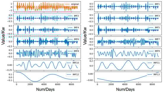
Figure 1.
Decomposition of the dataset using EMD.
2.1.3. Fluctuation analysis
Fluctuation analysis can obtain reliable long-range correlation series. In our method, fluctuation analysis is used to process the single IMF, which is decomposed by EMD. For each IMF, we can calculate the Hurst exponent through DFA, and it essentially indicates the long-range memory of a time series, which has an important role in capturing self-similar features [33]. The calculating process of the Hurst exponent is defined as follows:
For the original IMF time series , the time series is firstly split into segments . For every , calculate the mean value:
where is the value of segment , and then calculate the deviation sequence for each segment:
where is the new deviation sequence for each segment, are elements in each segment, is the mean values of each segment. Then, the widest difference is calculated for each deviation sequence:
where is the widest difference of each deviation sequence. The standard deviation was then calculated for each segment:
where is the standard deviation, which was used to calculate values:
For each segmentation method, there are different segmentation size , the values of the individual segments were averaged to obtain :
Thus, and will be obtained, and the relationship between and can reflect long-range memory of a time series. and are linearly correlated:
where is the Hurst exponent, which varies with the number of dividing windows; is defaulted to in our method. For each , we calculate the Hurst exponent in order to analyze the fluctuation trend, the is used to divide whether there is a positive correlation or inverse correlation. For given , the long-range positive correlation series and long-range inverse correlation series can be defined as follows:
where is the number of , and means is a positive correlation, means is a inverse correlation.
2.2. Long Short-Term Memory
The long short-term memory (LSTM) structure is a variant of recurrent neural networks (RNN) that integrates multiple memory units to effectively oversee and regulate information by employing a set of three gate mechanisms: the input gate, the forget gate, and the output gate [34]. After LSTM was proposed, it has been the most popularly used supervised deep learning algorithm [35]. For a given time series , the LSTM network can be expressed as follows:
where is the input, is the hidden state, , , and represent the input gate, forget gate, and output gate, respectively. is the cell state. is the candidate cell state. , , , and are the input weight matrices. , , , and are the biases of LSTM cell.
2.3. Framework
The framework of EMDHM is presented in Figure 2. It contains two main parts: the decomposition part and the forecasting part. In the first part of EMDHM, known as DEMDFA, it detrends the linear trend and periodic trend from the original load series using a linear function and a trigonometric function, which fit the curve sequentially. The other component is called long-range correlation series, and it will be decomposed into IMFs by using EMD. For every decomposed IMF, DEMDFA employs fluctuation analysis to determine whether an IMF exhibits positive or inverse correlation by extracting its fluctuation features, and then it divides IMFs into LRPCS and LRICS, which contain the primary fluctuation information from high-frequency, sub-hourly load. Our method extracts four main components (four sub-series) from the original data, which is linear series, periodic series, LRPCS, and LRICS. In the second part of EMDHM, our method introduces two LSTMs to model LRPCS and LRICS separately, and subsequently predict two long-range correlation series. Linear and trigonometric functions are utilized to forecast the linear and periodic components, respectively. Finally, all these series are ensembled to produce the final forecasting result.
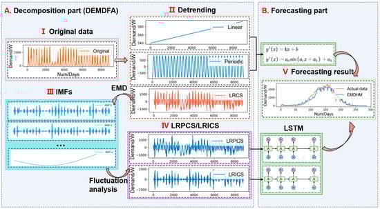
Figure 2.
The framework of EMDHM.
3. Results and Discussions
This section presents two cases designed to validate the performance of EMDHM. In the first case, we use the PV dataset as the test dataset to demonstrate the positive impact of the sub-series decomposed by the novel decomposition algorithm on predicted results, as well as the prediction improvement achieved by combining LSTM with DEMDFA in EMDHM. We also compare the performance among different decomposition methods combined with LSTM, such as EMD-LSTM using empirical mode decomposition (EMD), SSA-LSTM based on singular spectrum analysis (SSA), and STL-LSTM based on seasonal and trend decomposition using loess (STL), to show EMDHM’s ability in minute load forecasting. In the second case, we conduct an experiment to predict hourly load series with varying sequence lengths. This is done to validate whether EMDHM’s decomposition algorithm consistently outperforms other algorithms in improving forecasting, regardless of whether the prediction length is short or long. What is more, we also aim to demonstrate the capability of EMDHM (containing the decomposition part of DEMDFA and the forecasting part) in both short-sequence and long-sequence hourly load forecasting. Further, the experiment is also designed to illustrate that our method exhibits better stability in comparison to other decomposition–ensemble methods, and the Panama Load dataset is used to evaluate the model’s performance in this experiment.
3.1. Evaluation Metrics
We introduce four evaluation metrics for measuring the performance of the model in our experiments: mean absolute error (MAE), root mean square error (RMSE), mean absolute range normalized error (MARNE), and R-squared (R2).
where is the length of the data, is the real data, is the prediction value, and is the average of the data.
3.2. Dataset Description
In our experiment, the PV dataset and the Panama load dataset are used, which have been published in papers [29,30]. The PV dataset contains PV power generation data recorded every 5 min from 1 July 2021 to 31 July 2021, with a total length of 8928. The Panama load dataset contains load demand data recorded every hour from 31 January 2015 to 9 April 2019, with a total length of 36,720. The features used to train models in our cases are detailed in Table 1. The curves of PV dataset and Panama load dataset are shown in Figure 3. Both the PV dataset and Panama load dataset are sub-hourly.

Table 1.
Features of the PV dataset and Panama load dataset.
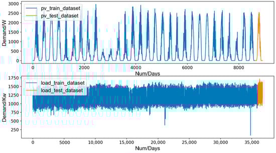
Figure 3.
The curves of PV dataset and Panama load dataset.
3.3. Case One: Model Performance in Forecasting PV Data
To validate the positive impact of sub-series decomposed by DEMDFA on predicted results and the effectiveness of the decomposition part (DEMDFA) of our method, EMDHM, when combined with the forecasting part (containing LSTM) as a decomposition–ensemble forecasting method, we designed case one. We firstly used 8640 data from the PV dataset as the training set to train models (including EMDHM, LSTM, EMD-LSTM, SSA-LSTM, and STL-LSTM), and then predicted the last 288 data; four evaluation metrics were introduced to show the performance differences. The prediction performances of each model are shown in Figure 4. For the fitting degree, the R2 value of LSTM is 0.893. Decomposition–ensemble methods like SSA-LSTM and STL-LSTM perform slightly better than a single LSTM, with R2 values of 0.899 and 0.901, respectively. However, EMD-LSTM does not fit the dataset well, with an R2 value of 0.832, significantly lower than other methods. This suggests that EMD has a negative impact on LSTM when applied to this dataset. EMDHM exhibits the highest performance in terms of goodness of fit, with a R2 value of 0.942, showing a 5.5% improvement over single LSTM and at least 0.041 higher than other decomposition–ensemble methods. This demonstrates that the sub-series decomposed by DEMDFA are effective in retaining information from original data. DEMDFA achieves greater improvement when combined with LSTM compared to other decomposition algorithms. Furthermore, the forecasting results of EMDHM exhibit significantly smaller errors when compared to actual data, with a MAE of 139.092, RMSE of 207.270, and MARNE of 0.053. Except for EMD-LSTM, which performs relatively poorly, the other two decomposition–ensemble models, SSA-LSTM and STL-LSTM, show smaller errors than the single LSTM, although the improvement is not as pronounced. SSA-LSTM only has a MAE improved by 1.7%, a RMSE improved by 2.8%, a MARNE improved by 2.9%. STL-LSTM has a MAE improved by 5.7%, a RMSE improved by 3.5%, a MARNE improved by 5.8%. The decomposition part of EMDHM, DEMDFA, extracts four main sub-series, which contain trend and long-range information. It not only detrends the original time series to achieve a reliable LRCS, but also simplifies complex LRCS by EMD and then analyzes fluctuation information to classify LRCS into LRPCS and LRICS. The four sub-series decomposed by DEMDFA contain enough information to be combined with LSTM, linear function, and trigonometric function, which results in improved forecasting performance. The MAE, RMSE, and MARNE of EMDHM are improved by 20.1%, 26.8%, and 22.1%, respectively, more than a single LSTM, which performs much better than other decomposition–ensemble methods in the experiment.
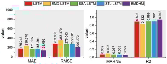
Figure 4.
Performances of each model in case one.
Analyzing the forecasting curves of each method (as shown in Figure 5), we can clearly observe that EMDHM outperforms the others in the section where value grows rapidly. In other sections, the distinctions between our method and other methods are less noticeable. However, the other four methods exhibit nearly identical curves in the growing section of power, which fail to capture the rapidly changing information in minute load series, leading to significant errors when fitting the actual data. Although other models struggle to fit the growing section effectively, EMDHM, being based on detrending, introduces a periodic sub-series to describe periodic information. In this dataset, since the PV data are strongly correlated with time, temperature, humidity, and some other features, it exhibits a very strong periodic behavior, with power peaks occurring at noon. Consequently, PV data resemble the shape of a trigonometric function. When dealing with such rapid value growth, the trigonometric-shaped periodic sub-series plays a crucial role in smoothing the forecasting curve (refer to Figure 6). Consequently, PV data resemble the shape of a trigonometric function. In our experiment, we observed that LSTM and conventional decomposition–ensemble methods struggled to capture such a rapidly growing trend due to limitations in their models. The superiority of EMDHM in such periodic load series is attributed to the presence of the periodic component.
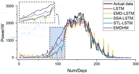
Figure 5.
Forecasting curves of each model in case one.
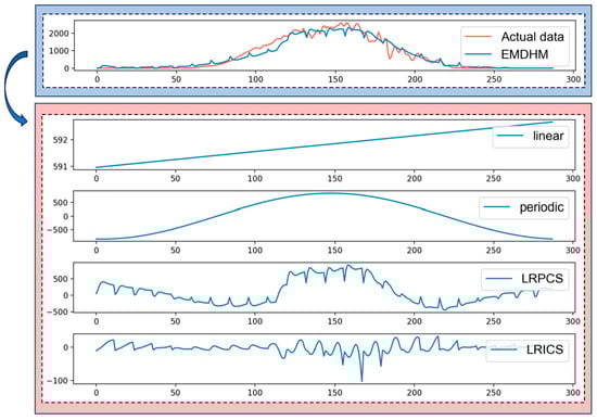
Figure 6.
Different components of the EMDHM forecasting curve.
Furthermore, upon analyzing the curve of EMD-LSTM, which performed the worst in this experiment, we identified that the reason for its high error lies in the excessively large fluctuations that hinder it from fitting the actual data curve effectively. However, our method maintains fluctuations within an appropriate range. By capturing fluctuation information through long-range correlation sub-series, our method fits high-frequency hourly load well and does not deviate too much from the original curve. Thus, when facing forecasting tasks involving load series with clear trends or high-frequency characteristics in the curve, it is reasonable to employ EMDHM for decomposition and subsequently forecast sub-hourly load curves. The experiment strongly demonstrates the positive impact of the sub-series decomposed by DEMDFA on predicted results and the effectiveness of our proposed model, EMDHM.
3.4. Case Two: Model Performance in Forecasting Panama Load Data
To demonstrate the comprehensiveness of EMDHM in forecasting sub-hourly load series and to assess its performance compared to other methods across various sequence lengths, we utilized Panama load data as test data to evaluate the forecasting performance of each model. The load data were sampled hourly. In the experiment, we analyzed the performance of each model at forecasting sequence lengths of 2 days (length 48), 4 days (length 96), 7 days (length 168), 14 days (length 336), and 30 days (length 720). This analysis aims to illustrate that our method not only outperforms other models in short-sequence prediction but also exhibits promising performance that surpasses other decomposition–ensemble methods in long-sequence prediction. The experiment presents EMDHM’s performance in long-sequence, sub-hourly load forecasting remains to be stable as the length of the sequence increases.
Table 2 and Table 3 show the MAE, RMSE, MARNE, and R2 of each model in hourly load forecasting. Upon analyzing the results for a sequence length of 48, EMDHM demonstrates its forecasting capabilities with a 20.0% decrease in MAE compared to SSA-LSTM (the best-performing model among the rest when predicting at length 48). It also achieves a 19.7% reduction in RMSE, a 16.7% decrease in MARNE, and a 0.9% increase in R2. For a prediction length of 96, it also performs well. In comparison to LSTM, the MSE is improved by 15.9%, the RMSE is improved by 19.3%, the MARNE is improved by 15% and the R2 is improved by 1.7%. These results highlight the superiority of MARNE’s framework, which combines the decomposition algorithm DEMDFA with LSTM, linear function, and trigonometric function, over a single LSTM. When the prediction length increases to 168, EMDHM continues to deliver the best fitting results, with an MAE of 32.742, RMSE of 39.220, MARNE of 0.020, and R2 of 0.960. The decomposition algorithm DEMDFA in EMDHM combines EMD for simplifying complex long-range series and DFA for signifying high-frequency series and fluctuation information, which consistently results in superior performance compared to other methods. Because of its linear component, periodic components, and long-range correlation components, it is stable though the prediction length becomes longer. Compared to the best metrics of other models, our method exhibits a remarkable performance improvement when the prediction length increases to 336. It achieves a 18.1% decrease in MAE, a 19.7% reduction in RMSE, a 15.4% decrease in MARNE, and a 2.7% increase in R2. What is more, the true superiority of EMDHM becomes fully evident when the prediction length reaches 720. Its MAE, RMSE, MARNE, and R2 are 34.3%, 30.2%, 35.3%, and 7.7% better than the corresponding best metrics of the other models. In the experiment, we find that our method remains stable in predicting hourly load series and performs well across different sequence lengths. From a sequence length of 48 to a length of 720, its fitting capability is consistently maintained at a high level. The R2 value only decreases by 4.7% compared to the initial value (whereas LSTM decreases by 13.6%, EMD-LSTM by 12.5%, SSA-LSTM by 10.7%, and STL-LSTM by 12.8%).
Table 2.
MAE and RMSE of each model in load forecasting.
Table 3.
MARNE and R2 of each model in load forecasting.
Upon analyzing the forecasting curves for prediction lengths of 48 and 96 (refer to Figure 7), we initially observe that EMDHM outperforms other methods in certain rapidly changing sections. Although all the methods exhibit good fitting when the prediction lengths are 48 and 96, EMDHM achieves lower errors due to its superior signifying capability in this fluctuation information. In short-sequence forecasting, STL-LSTM is the worst method for fitting actual data, and experiments indicate that STL has a negative effect on improving LSTM in this prediction length. The other two decomposition algorithms, EMD and SSA, have a minor positive impact on improving the fitting accuracy of LSTM. However, EMDHM clearly demonstrates the utility of its decomposition algorithm and exhibits an obviously positive effect on combining LSTM by effectively capturing high-frequency and long-range correlation information. Thus, our method excels at fitting rapid fluctuations and maintains a higher R2 level in short-sequence forecasting.
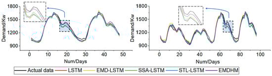
Figure 7.
Forecasting curves when prediction lengths are 48 and 96.
Similar situations are observed in the forecasting curves when the prediction lengths are 168 and 336 (refer to Figure 8). What is more, EMDHM’s curve also fits the actual data well in the domain of extrema, which is common in high-frequency, sub-hourly loads. When the load demand curves reach their extrema, the forecasting curves of EMDHM demonstrate the best fit with the actual data compared to other models. When encountering local maxima, our method’s prediction values increase by capturing extrema information. Similarly, when local minima are encountered, it can also capture them in a timely manner to adjust the prediction values. Consequently, the results additionally demonstrate our method’s excellent performance in fitting high-frequency and rapidly changing sub-hourly load curves.
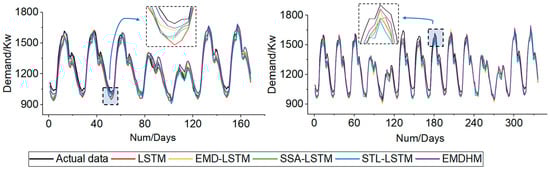
Figure 8.
Forecasting curves when prediction lengths are 168 and 336.
In long-sequence forecasting with a prediction length of 720 (refer to Figure 9), single LSTM and other decomposition-based LSTMs struggle to effectively capture high-frequency and rapidly changing hourly load series. The highest R2 achieved is only 0.869, which remains significantly lower than the performance of our method. Upon analyzing the results, we find that employing decomposition algorithms in long-sequence forecasting can enhance the fitting accuracy of machine learning model. DEMDFA exhibits the most significant improvement, with EMDHM’s MAE improving by 42.8%, RMSE improving by 37.9%, MARNE improving by 43.6%, and R2 improving by 12.1%. The significant series decomposition capability of EMDHM enables it to exhibit remarkable forecasting ability, irrespective of the prediction length, in the forecasting part. The characteristics of proposed decomposition algorithm DEMDFA can be summarized as trend, periodicity, long-range, and stability. Therefore, case two confirms the applicability of our method in both short- and long-sequence, sub-hourly load forecasting.
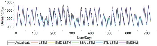
Figure 9.
Forecasting curve when prediction length is 720.
4. Conclusions
This paper proposes a decomposition algorithm, DEMDFA, used for properly decomposing sub-hourly load series with high frequencies and further introduces a decomposition–ensemble method, EMDHM, to improve the forecasting of sub-hourly load curves. To obtain a reliable long-range correlation series from high-frequency data and prevent the false detection of long-range correlation caused by strong trends in the original data, our proposed method, namely EMDHM, first detrends the linear and periodic trends from the original series, retaining the Long-Range Correlation Series (LRCS). Due to the complexity of Long-Range Correlation Series (LRCS), the effective method of load decomposition, EMD, is employed to decompose the remaining series, thereby obtaining IMFs with independent information. Next, EMDHM analyzes the fluctuations in the individual IMFs, dividing them into LRPCS and LRPIS components. Containing LSTM into its forecasting part, EMDHM shows DEMDFA’s significant improving in LSTM by designing two cases using the PV dataset and the Panama load dataset, and its enhancing effect surpasses that of other decomposition methods when combined with LSTM for sub-hourly load prediction. Based on the experiments, the conclusion can be summarized as follows:
- The sub-series decomposed by DEMDFA plays a crucial role in predicting the results. EMDHM performs exceptionally well in sub-hourly load forecasting. When predicting PV power series, it exhibits the best performance among the models, with MAE, RMSE, MARNE, and R2 values of 139.092, 207.270, 0.053, and 0.942, respectively. This represents an improvement of 20.1% in MAE, 26.8% in RMSE, 22.1% in MARNE, and 5.4% in R2 compared to single LSTM, and it significantly outperforms other decomposition–ensemble methods.
- EMDHM presents enhanced stability in both short- and long-sequence forecasting. In sub-hourly load forecasting, because of DEMDFA’s characteristics of trend, periodicity, long-range, and stability, the extracted series provide distinct information. Thus, EMDHM’s fitting capability remains consistently high regardless of changes in the prediction length. Its R2 value only decreases by 4.7% when the prediction length varies from 48 to 720, compared to the decreases of 13.6% for LSTM, 12.5% for EMD-LSTM, 10.7% for SSA-LSTM, and 12.8% for STL-LSTM. Furthermore, the performance of EMDHM remains the best in our experiment, especially when the prediction length is 720. Compared to the best metrics of the other four methods, our method’s MAE, RMSE, MARNE, and R2 are superior by 34.3%, 30.2%, 35.3%, and 7.7%, respectively. This highlights the robust decomposition stability of DEMDFA and EMDHM’s significant performance.
This paper proposes a decomposition algorithm DEMDFA to decompose sub-hourly load series and further introduce a decomposition–ensemble method EMDHM. Our experiments prove that EMDHM’s applicability of sub-hourly load forecasting. However, we observed that EMDHM also exhibits fluctuations when predicting load curves that remain stable. Therefore, it may not perform well in relatively stable sections, leading to increased errors. As a result, we will conduct further studies to investigate the reasons for these fluctuations and consider smoothing them after trying to recognize these sections to improve its performance in our future work. In addition, transfer learning, as a deep learning method, has achieved significant results in load forecasting research [36,37]. Therefore, we also consider introducing transfer learning methods in our future work.
Author Contributions
Writing and methodology, C.Y.; supervision, N.W. and F.Z.; visualization, J.W. and C.R.; software, X.L. All authors have read and agreed to the published version of the manuscript.
Funding
This research was funded by the National Key R&D Program of China (No. 2021YFB3101700), the National Natural Science Foundation of China (No. 62002078), the Project of Guangzhou Association for Science and Technology (No. 202201010609), and the Young Talent Support Project of Guangzhou Association for Science and Technology (No. QT20220101122).
Data Availability Statement
The data presented in this study are openly available in reference number [29,30].
Conflicts of Interest
The authors declare no conflicts of interest.
Abbreviations
| EMDHM | Empirical mode decomposition-based hybrid model |
| STLF | Short-term load forecasting |
| AI | Artificial intelligence |
| ARIMA | Auto regressive integrated moving average |
| ANN | Artificial neural network |
| LSTM | Long short-term memory |
| RNN | Recurrent neural network |
| MVMD | Multivariate variational mode decomposition |
| EMD | Empirical mode decomposition |
| GRU | Gate recurrent unit |
| IMF | Intrinsic mode function |
| PV | Photovoltaic |
| DFA | Detrend fluctuation analysis |
| SSA | Singular spectrum analysis |
| DEMDFA | Detrended empirical mode decomposition for fluctuation analysis |
| LRCS | Long-range correlation series |
| LRPCS | Long-range positive correlation series |
| LRICS | Long-range positive correlation series |
| MAE | Mean absolute error |
| MAPE | Mean absolute percentage error |
| MARNE | Mean Absolute Range Normalized Error |
| RMSE | Root mean square error |
| R2 | R-squared |
References
- Feinberg, E.A.; Genethliou, D. Load Forecasting. In Proceedings of the Load Forecasting, Workshop on Applied Mathematics for Deregulated Electric Power Systems, Arlington, VA, USA, 3–4 November 2003; pp. 269–285. [Google Scholar]
- Hippert, H.S.; Pedreira, C.E.; Souza, R.C. Neural networks for short-term load forecasting: A review and evaluation. IEEE Trans. Power Syst. 2001, 16, 44–55. [Google Scholar] [CrossRef]
- Bilgic, M.; Girep, C.P.; Aslanoglu, S.Y.; Aydinalp-Koksal, M. Forecasting Turkey’s short term hourly load with artificial neural networks. In Proceedings of the IEEE PES T&D 2010, New Orleans, LA, USA, 19–22 April 2010; pp. 1–7. [Google Scholar]
- Dou, Y.; Zhang, H.; Zhang, A. An Overview of Short-term Load Forecasting Based on Characteristic Enterprises. In Proceedings of the 2018 Chinese Automation Congress (CAC), Xi’an, China, 30 November–2 December 2018; pp. 3176–3180. [Google Scholar]
- Khodaei, A.; Shahidehpour, M.; Bahramirad, S. SCUC With Hourly Demand Response Considering Intertemporal Load Characteristics. IEEE Trans. Smart Grid 2011, 2, 564–571. [Google Scholar] [CrossRef]
- Kwac, J.; Flora, J.; Rajagopal, R. Household Energy Consumption Segmentation Using Hourly Data. IEEE Trans. Smart Grid 2014, 5, 420–430. [Google Scholar] [CrossRef]
- Wei, N.; Li, C.J.; Peng, X.L.; Zeng, F.H.; Lu, X.Q. Conventional models and artificial intelligence-based models for energy consumption forecasting: A review. J. Pet. Sci. Eng. 2019, 181, 106187. [Google Scholar] [CrossRef]
- Moghram, I.; Rahman, S. Analysis and evaluation of five short-term load forecasting techniques. IEEE Trans. Power Syst. 1989, 4, 1484–1491. [Google Scholar] [CrossRef]
- Papalexopoulos, A.D.; Hesterberg, T.C. A regression-based approach to short-term system load forecasting. IEEE Trans. Power Syst. 1990, 5, 1535–1547. [Google Scholar] [CrossRef]
- Contreras, J.; Espinola, R.; Nogales, F.J.; Conejo, A.J. ARIMA models to predict next-day electricity prices. IEEE Trans. Power Syst. 2003, 18, 1014–1020. [Google Scholar] [CrossRef]
- Park, D.C.; El-Sharkawi, M.A.; Marks, R.J.; Atlas, L.E.; Damborg, M.J. Electric load forecasting using an artificial neural network. IEEE Trans. Power Syst. 1991, 6, 442–449. [Google Scholar] [CrossRef]
- Liu, C.; Jin, Z.J.; Gu, J.; Qiu, C.M. Short-Term Load Forecasting using A Long Short-Term Memory Network. In Proceedings of the IEEE PES Innovative Smart Grid Technologies Conference Europe (ISGT-Europe), Torino, Italy, 26–29 September 2017. [Google Scholar]
- Zheng, H.; Yuan, J.; Chen, L. Short-Term Load Forecasting Using EMD-LSTM Neural Networks with a Xgboost Algorithm for Feature Importance Evaluation. Energies 2017, 10, 1168. [Google Scholar] [CrossRef]
- Reis, A.J.R.; da Silva, A.P.A. Feature extraction via multiresolution analysis for short-term load forecasting. IEEE Trans. Power Syst. 2005, 20, 189–198. [Google Scholar]
- Huang, H.; Chen, J.; Sun, R.; Wang, S. Short-term traffic prediction based on time series decomposition. Phys. A Stat. Mech. Its Appl. 2022, 585, 126441. [Google Scholar] [CrossRef]
- Wang, Z.; Chen, L.; Chen, H.; Rehman, N.u. Monthly ship price forecasting based on multivariate variational mode decomposition. Eng. Appl. Artif. Intell. 2023, 125, 106698. [Google Scholar] [CrossRef]
- Wei, Y.; Chen, Z.; Zhao, C.; Tu, Y.; Chen, X.; Yang, R. A BiLSTM hybrid model for ship roll multi-step forecasting based on decomposition and hyperparameter optimization. Ocean. Eng. 2021, 242, 110138. [Google Scholar] [CrossRef]
- Qiu, X.H.; Ren, Y.; Suganthan, P.N.; Amaratunga, G.A.J. Empirical Mode Decomposition based ensemble deep learning for load demand time series forecasting. Appl. Soft Comput. 2017, 54, 246–255. [Google Scholar] [CrossRef]
- Li, G.; Zhong, X. Parking demand forecasting based on improved complete ensemble empirical mode decomposition and GRU model. Eng. Appl. Artif. Intell. 2023, 119, 105717. [Google Scholar] [CrossRef]
- Zhu, B.; Han, D.; Wang, P.; Wu, Z.; Zhang, T.; Wei, Y.-M. Forecasting carbon price using empirical mode decomposition and evolutionary least squares support vector regression. Appl. Energy 2017, 191, 521–530. [Google Scholar] [CrossRef]
- Wang, J.J.; Zhang, W.Y.; Li, Y.N.; Wang, J.Z.; Dang, Z.L. Forecasting wind speed using empirical mode decomposition and Elman neural network. Appl. Soft Comput. 2014, 23, 452–459. [Google Scholar] [CrossRef]
- Fan, C.; Ding, C.; Zheng, J.; Xiao, L.; Ai, Z. Empirical Mode Decomposition based Multi-objective Deep Belief Network for short-term power load forecasting. Neurocomputing 2020, 388, 110–123. [Google Scholar] [CrossRef]
- Gonzalez-Romera, E.; Jaramillo-Moran, M.A.; Carmona-Fernandez, D. Monthly Electric Energy Demand Forecasting Based on Trend Extraction. IEEE Trans. Power Syst. 2006, 21, 1946–1953. [Google Scholar] [CrossRef]
- Kantelhardt, J.W.; Koscielny-Bunde, E.; Rego, H.H.A.; Havlin, S.; Bunde, A. Detecting long-range correlations with detrended fluctuation analysis. Phys. A Stat. Mech. Its Appl. 2001, 295, 441–454. [Google Scholar] [CrossRef]
- Auno, S.; Lauronen, L.; Wilenius, J.; Peltola, M.; Vanhatalo, S.; Palva, J.M. Detrended fluctuation analysis in the presurgical evaluation of parietal lobe epilepsy patients. Clin. Neurophysiol. 2021, 132, 1515–1525. [Google Scholar] [CrossRef] [PubMed]
- Zhu, J.; Li, M.; Luo, L.; Zhang, B.; Cui, M.; Yu, L. Short-term PV power forecast methodology based on multi-scale fluctuation characteristics extraction. Renew. Energy 2023, 208, 141–151. [Google Scholar] [CrossRef]
- Wei, N.; Yin, L.H.; Li, C.; Wang, W.; Qiao, W.B.; Li, C.J.; Zeng, F.H.; Fu, L.D. Short-term load forecasting using detrend singular spectrum fluctuation analysis. Energy 2022, 256, 124722. [Google Scholar] [CrossRef]
- Wei, N.; Li, C.; Peng, X.; Li, Y.; Zeng, F. Daily natural gas consumption forecasting via the application of a novel hybrid model. Appl. Energy 2019, 250, 358–368. [Google Scholar] [CrossRef]
- Al-Ja’afreh, M.A.A.; Mokryani, G.; Amjad, B. An enhanced CNN-LSTM based multi-stage framework for PV and load short-term forecasting: DSO scenarios. Energy Rep. 2023, 10, 1387–1408. [Google Scholar] [CrossRef]
- Aguilar Madrid, E. Short-term electricity load forecasting (Panama case study). Mendeley Data 2021, V1. [Google Scholar] [CrossRef]
- Huang, N.; Shen, Z.; Long, S.; Wu, M.L.C.; Shih, H.; Zheng, Q.; Yen, N.-C.; Tung, C.-C.; Liu, H. The empirical mode decomposition and the Hilbert spectrum for nonlinear and non-stationary time series analysis. Proc. R. Soc. Lond. Ser. A Math. Phys. Eng. Sci. 1998, 454, 903–995. [Google Scholar] [CrossRef]
- Huang, N.E.; Shen, Z.; Long, S.R. A New View of Nonlinear Water Waves: The Hilbert Spectrum. Annu. Rev. Fluid Mech. 1999, 31, 417–457. [Google Scholar] [CrossRef]
- Hurst, H.E. Long-Term Storage Capacity of Reservoirs. Trans. Am. Soc. Civ. Eng. 1951, 116, 770–799. [Google Scholar] [CrossRef]
- Kong, W.; Dong, Z.Y.; Jia, Y.; Hill, D.J.; Xu, Y.; Zhang, Y. Short-Term Residential Load Forecasting Based on LSTM Recurrent Neural Network. IEEE Trans. Smart Grid 2019, 10, 841–851. [Google Scholar] [CrossRef]
- Malhotra, A.; Jindal, R. Deep learning techniques for suicide and depression detection from online social media: A scoping review. Appl. Soft Comput. 2022, 130, 109713. [Google Scholar] [CrossRef]
- Wei, N.; Yin, C.; Yin, L.; Tan, J.; Liu, J.; Wang, S.; Qiao, W.; Zeng, F. Short-term load forecasting based on WM algorithm and transfer learning model. Appl. Energy 2024, 353, 122087. [Google Scholar] [CrossRef]
- Wei, N.; Yin, L.; Yin, C.; Liu, J.; Wang, S.; Qiao, W.; Zeng, F. Pseudo-correlation problem and its solution for the transfer forecasting of short-term natural gas loads. Gas Sci. Eng. 2023, 119, 205133. [Google Scholar] [CrossRef]
Disclaimer/Publisher’s Note: The statements, opinions and data contained in all publications are solely those of the individual author(s) and contributor(s) and not of MDPI and/or the editor(s). MDPI and/or the editor(s) disclaim responsibility for any injury to people or property resulting from any ideas, methods, instructions or products referred to in the content. |
© 2024 by the authors. Licensee MDPI, Basel, Switzerland. This article is an open access article distributed under the terms and conditions of the Creative Commons Attribution (CC BY) license (https://creativecommons.org/licenses/by/4.0/).