Article

Does Green Finance Improve Industrial Energy Efficiency? Empirical Evidence from China

1
College of Energy Engineering, Xi’an University of Science and Technology, Xi’an 710054, China
2
School of Economics and Management, Yan’an University, Yan’an 716000, China
3
Soft Science Research Base for Green and Low-Carbon Development of Energy Industry in Shaanxi Province, Yan’an University, Yan’an 716000, China
*
Author to whom correspondence should be addressed.
Energies 2024, 17(19), 4818; https://doi.org/10.3390/en17194818
Submission received: 16 August 2024 / Revised: 10 September 2024 / Accepted: 23 September 2024 / Published: 26 September 2024

Abstract

:
Improving industrial energy efficiency (IEE) is crucial for reducing CO2 emissions. Green finance (GF) provides an essential economic instrument for investment in IEE improvement. However, previous studies have not reached a consensus on whether GF can promote energy efficiency. In addition, more research is needed in the industrial sector. Therefore, this study focused on the industrial level to investigate GF’s impact on IEE and its heterogeneity using a two-way fixed effects model. The moderating effect, threshold effect, and spatial lag models were used to test the various effects of GF on IEE. In addition, the spatial clustering characteristics of IEE were analyzed. The results indicate the following: GF can significantly promote IEE, positively improves IEE in the central and eastern areas, and has a negative impact in the western area; the marketization level (ML) is an important channel through which GF can further improve IEE; GF’s impact on IEE exhibits a single threshold effect of the level of economic development (EDL) and green credit (GCL); GF promotes local IEE improvement but prevents neighboring IEE improvement; and IEE shows four types of clusters, but only in about one-third of the provinces. Based on these results, several recommendations are provided.

Graphical Abstract

1. Introduction

With economic growth and urbanization, energy issues are becoming particularly important. In China, energy carbon emissions account for 80% of total carbon emissions [1], seriously hindering the achievement of the ‘double carbon’ goals. Previous studies have shown that the reduction in China’s carbon emissions will be dominated by energy efficiency improvements before carbon peaks in 2030, contributing over 60% of the reduction [2]. Yu et al. [3] calculated that the energy efficiency in advanced and emerging economies is low, averaging 0.44. Energy efficiency refers to the ratio of energy output to energy input [4]. Improving energy efficiency means obtaining more energy output with as little energy input as possible, which will reduce fossil fuel consumption and contribute to the realization of the “double carbon” goals [5]. Industry is a high-energy-consuming, polluting, and high-emission sector in China. At the end of 2021, industrial energy consumption still accounted for 66.75% of China’s total energy consumption [6]. The IEE in China represents about CNY 95 million/10,000 tons of standard coal, and there is still capacity for further improvement [6]. Therefore, it is urgent to reduce energy consumption in all areas of industry, thereby reducing industrial CO2 emissions. However, improving IEE requires a significant amount of capital investment [7]. In addition to government investment, it is necessary to fully utilize market-oriented instruments such as GF to solve the funding shortage problem.
GF can balance economic growth, environmental protection, and sustainable development [8]. GF provides a financial service for investment, financing, operations, risk management, and others for environmental protection, energy conservation, and clean energy projects [9] to realize environmentally sustainable economic development [10]. Green financial products principally comprise green credit, bonds, insurance, investment, and carbon finance [11]. The essence of GF is to use those instruments to promote the transfer of funds to energy conservation and environmental protection, thereby reducing the dependence of economic activities on fossil fuels [12]. For the Chinese industry, GF currently principally provides green capital investment for clean production projects such as green upgrading and the renovation of industrial parks [13], green low-carbon and high-efficiency equipment manufacturing projects, clean energy industry projects such as the clean and efficient utilization of traditional energy, and the efficient operation of energy systems, thereby promoting industrial low-carbon transition. However, due to the limitations in data and information availability, there is currently no publicly available evidence to confirm whether and to what extent GF has actually played a role in these green projects. Azhgaliyeva et al. [14] believes that the Association of South-East Asian Nations’ green bond policy might not necessarily be effective in promoting energy efficiency projects, as its green bonds can be used to refinance past loans. The promoting role of GF in the industrial low-carbon transition process has not been fulfilled.
Under the above circumstances, much academic research has been conducted on GF, energy efficiency, and the relationship between the two. Among the studies, in terms of GF measurement, some scholars have used a single indicator or a fusion degree of two indicators to measure GF [10,15]; however, these cannot comprehensively and effectively measure the level of GF. Scholars have gradually recognized the necessity for a GF indicator system to measure the level of GF [8,11,16]. In terms of energy efficiency measurement, scholars have usually strived to use a one-dimensional indicator for measurement purposes, including, for example, energy macro-efficiency (the inverse of energy intensity) [17], energy thermodynamic efficiency (energy’s thermal efficiency) [18], energy physical efficiency (energy consumption per unit of product or process) [19], and energy value efficiency (energy input and output measured by value quantity) [5]. Some scholars have also used total factor energy efficiency [20] or energy return on investment (EROI) to measure energy utilization efficiency [21]. When calculating the overall energy efficiency level of a country, region, or industry, scholars have often used macro energy efficiency, which is the reciprocal of energy intensity [17].
In terms of the relationship between the two, scholars have not currently reached a consensus on whether GF can promote energy efficiency. Some experts have found that GF can promote improvements in IEE. For example, Guo et al. [20] used the spatial Durbin model (SDM) to study the GF’s impact on total factor energy efficiency. They found that GF positively affects energy efficiency, and Internet development and ER can help GF to further improve energy efficiency. Lee and Lee adopted a two-way fixed effects model to study GF’s impact on green total factor productivity (GTFP). They also concluded that GF significantly improves green productivity [22]. Lee and Wang [23] used the fixed effects model to study GF’s impact on energy efficiency, and found that GF significantly contributes to energy efficiency. Xu et al. [24] used the same model as Lee and Wang [23] to study GF’s impact on GTFP. They found that GF positively promotes GTFP. Tan et al. [25] adopted a difference-in-differences model to study the green credit policy on energy efficiency of 36 sectors in China, and found that it could improve energy efficiency. Liu et al. [26] found that GF was a highly supportive financing tool for energy efficiency of E7 economies. However, some experts believe that GF cannot promote energy efficiency. For instance, Wang et al. [27] used the Tobit model to study GF’s impact on China’s regional energy efficiency. They concluded that GF cannot promote energy efficiency nationally and has a regional heterogeneity. Yu et al. [3] used the same model as Xu et al. [24] to study GF’s impact on the energy efficiency of developing and developed economies. They found that GF negatively affects energy efficiency. Hou et al. [28] used the panel autoregressive distributed lag model to study the nexus between GF, Fintech, and energy efficiency of 10 Asian economies. They found that Fintech negatively affects energy efficiency, and increasing GF leads to a decline in energy efficiency in the long run. In addition, Meng et al. [29] used the generalized method of moments (GMMs) system to study GF’s impact on energy efficiency. They agreed that GF and energy efficiency had a positive U-shaped relationship. In addition, only a few scholars have included some moderating variables in their research on direct effects to study how these variables moderate GF’s effect on energy efficiency [20]. In summary, scholars have focused on GF’s impact on energy efficiency at the macro level, but little research exists on the relationship between the two in the industrial field. Moreover, there are more studies on China and fewer comparative studies on other countries and regions. Also, econometric methods are commonly used for empirical testing. Regarding the research viewpoint, scholars have yet to reach a consensus on the relationship between the two.
Therefore, the question arises as to whether GF promotes energy efficiency improvement in the industrial sector? If this is correct, then how strong is that effect? Moreover, further research is still required, such as that on the impact of heterogeneity, moderating effects, nonlinear effects, and spatial spillover effects of GF on IEE. In light of this, to further test the relationships between GF and IEE, we selected the panel data from the period 2005–2020 from 30 of China’s provinces to investigate GF’s direct impact, heterogeneity, and other various effects on IEE and the spatial clustering characteristics of IEE. In this study, we aim to clarify the mechanisms of GF that affect IEE to help accelerate China’s industrial green low-carbon transition process and provide a reference for optimizing relevant policy design and experience for other countries or regions to use GF to promote IEE improvement.
This study has made several contributions. First, based on an industrial level, the effects of GF on IEE are clarified, which has complemented the theoretical study of GF’s effects on energy efficiency. Second, the regional heterogeneity, moderating, nonlinear, and spatial spillover effects of GF on IEE are verified through empirical tests, which have enriched the existing studies [20,27,30], and provide empirical evidence for GF’s improving effects on IEE. Third, the spatial clustering characteristics of IEE on the map are also taken into account using ArcGIS 10.8 software. Such results will help us to develop more effective policy measures to improve IEE.
The study is organized as follows. The next section presents the theoretical hypotheses. Section 3 describes the methodology, which mainly includes the main models, variables, processing explanations, and data sources. Figure 1 shows the methodological framework of this paper. Section 4 summarizes and analyzes the main research findings while conducting robust tests. Section 5 discusses the policy recommendations. In Section 6, the conclusions are provided.

2. Theoretical Hypotheses

2.1. Mechanism of the Direct Impact of GF on IEE

Some researchers have confirmed that GF can improve energy efficiency [20,31] and helps to control energy consumption, and it is argued that GF achieves this through lowering energy consumption and minimizing reliance on fossil fuels [12]. Moreover, GF improves energy efficiency by controlling the credit direction and scale [20], and enables the incorporation of sustainable environmental development and low-carbon economic principles into financial investment. In turn, this can provide funding support for green and efficient energy projects of industrial enterprises while forcing energy-intensive and polluting industries to accelerate the green and low-carbon transition and upgrading, thereby affecting the IEE. Hence, Hypothesis 1 is formulated.
Hypothesis 1.
GF positively improves IEE.

2.2. Mechanism of the Marketization Level (ML) on the Impact of GF on IEE

The ML can help GF further improve IEE. Guo et al. [20] found that GF could improve energy efficiency. Xu et al. [24] also found that GF could promote GTFP. When the ML is high, the degree of direct government intervention is relatively low [32], and it becomes easier to break the market access threshold [33]. The circulation speed of resources and elements is faster. Market competition is more intense, the green financial system is more mature [34], and industrial enterprises can quickly obtain green financing and loans to improve efficiency further. Accordingly, Hypothesis 2 is formulated.
Hypothesis 2.
ML moderates GF’s impact on IEE.

2.3. Mechanism of the Nonlinear Effect of GF on IEE

According to the level of economic development (EDL), GF’s impact on environmental quality has been shown as presenting an inverted U-shaped relationship [8]. Lee and Lee concluded that the positive effect of GF on GTFP is more significant in regions with higher economic and social development levels [22]. Zhang et al. [17] agreed that GF is more effective in reducing haze pollution by improving energy efficiency in areas that already have a high GF level. Yin et al. [35] found that the higher the level of GF is in an area, the greater the promotional effect of ER is on green technological innovation. Wang et al. [27] concluded that GF improved energy efficiency in the eastern area, inhibited the central area’s energy efficiency, and had no relationship in the western area. This may be because of the different economic and GF development stages and levels. For the same region, it can be inferred that, when its EDL and GF levels are at different stages of development, GF’s impact on energy efficiency may be different, and a nonlinear relationship may occur. Lan et al. [36] concluded that GF and industrial pollutant emissions had an inverted N-shaped relationship, and Meng et al. [29] identified that GF and energy efficiency had a positive U-shaped relationship. That is, when the level of GF is low, it inhibits energy efficiency improvement; however, as the level of GF increases, it significantly promotes energy efficiency improvement. Moreover, GF is mainly financed through loans to industrial enterprises [37]; therefore, the level of green credit (GCL) is chosen as a proxy variable for GF in each province to test the nonlinear relationship between GF and IEE. Hence, Hypothesis 3 is proposed.
Hypothesis 3.
GF’s impact on IEE exhibits a nonlinear relationship due to EDL and GCL.

2.4. Spatial Spillover Effects of GF on IEE

In China, the interprovincial population size, resource endowment, and other significant differences [38] often lead to siphon or diffusion effects. The GF levels in different regions of China are different and show substantial spatial differences, agglomeration characteristics [16], and spatial spillover effects [39]. Energy efficiency in China also has a significant spatial positive autocorrelation, exhibiting high–high and low–low clusters [40]. Moreover, Wang et al. [39] discovered that, when GF’s level is high in a region, highly polluting and energy-consuming industries will choose to relocate to neighboring areas with a low green development level to avoid the additional costs of environmental pollution control [39]. However, this behavior also leads to a subsequent decline in the eco-efficiency of the neighboring provinces [41]. Guo et al. [20] identified that GF could improve the energy efficiency of both local and neighboring regions. When the local area effectively improves energy efficiency through GF and achieves sound energy-efficiency improvement effects, this will have a demonstrative effect, leading neighboring areas to imitate its practices. In addition, industry is a major energy consuming sector in China. Whether GF can also promote IEE in local and surrounding areas needs further verification. Thus, Hypothesis 4 is proposed.
Hypothesis 4.
GF has a spatial spillover effect on IEE.

3. Methods, Variables, and Data

3.1. Economic Models

3.1.1. Benchmark Regression Model

To empirically test GF’s impact on IEE and verify Hypothesis 1, we followed the method of Wu et al. [42] and constructed a benchmark regression model, as shown in Equation (1).
I E E i t = γ + β 1 G F i t + β C o n t r o l i t + μ i + δ t + ε i t
where I E E i t represents the IEE of the ith province in the t-th year; G F i t denotes the level of GF; C o n t r o l i t is a series of control variables; γ is a constant term; β and β 1 are coefficients to be estimated; μ i and δ t are the individual fixed and time fixed effects; and ε i t is a random disturbance term.
Furthermore, given that there may be endogeneity problems, with reference to Du et al. [9], we introduced a dynamic panel model and used the technique of the GMMs to evaluate the robustness of benchmark regression result, as shown in Equation (2).
I E E i t = γ + β 1 I E E i t 1 + β 2 G F i t + β C o n t r o l i t + μ i + δ t + ε i t

3.1.2. Moderating Effect Model

The change in ML may weaken or strengthen the impact of GF on IEE. Therefore, we drew on the approach of Baron and Kenny [43] and established a moderating effect model to verify the validity of Hypothesis 2, as shown in Equations (3) and (4).
IEE it = d + e G F i t + h M L i t + β C o n t r o l i t + μ i + δ t + ε i t
I E E i t = d + e G F i t + h M L i t + k G F i t M L i t + β C o n t r o l i t + μ i + δ t + ε i t
where Equation (3) is the main effect model; ML denotes the marketization level; Equation (4) is the moderating effect model; e and e are the coefficients of GF; h and h are the coefficients of ML; k is the moderating effect; and d and d are constant terms.

3.1.3. Threshold Effect Model

When EDL and GCL are at different stages in a region, this may lead to nonlinear relationships in GF’s impact on IEE. In this study, we relied on the work of Wang et al. [44] and constructed a threshold fixed effects model, with GCL and EDL as the threshold variables to verify the validity of Hypothesis 3, as detailed in Equation (5).
I E E i t = σ 0 + σ 1 G F i t I i t M i t θ 1 + σ 2 G F i t I i t M i t θ 2 + σ c X i t + ε i t
where M i t is the threshold variable, i.e., EDL or GCL; θ is the threshold value; and I   · is the indicator function, and its value is either 0 or 1.

3.1.4. Spatial Effect Model

To analyze the spatial clustering characteristics of IEE in each province of China at a more microscopic scale, we built the model using the approach of Yu et al. [45]. Equation (6) provides the calculation formulas of the Anselin Local Moran’s I.
I i = x i x ¯ j = 1 n w i j x j x ¯ s 2
where x i and x j represent the IEE of province i and j , respectively; x ¯ is the average IEE of all provinces; w i j is the partial weight matrix; n is the province number; and s = i = 1 n j = 1 n w i j [45].
The Moran’s I can only reflect the spatial clustering characteristics of IEE. To investigate whether there is a spatial spillover effect of GF on IEE and verify the validity of Hypothesis 4, we used methods such as the Lagrange multiplier (LM), Hausman, and likelihood ratio (LR) tests to determine which model would be used [20,39]. Equations (7)–(10) provide the formulas for the spatial lag model (SLM), spatial error model (SEM), and SDM.
I E E i t = ρ w i j I E E j t + β G F i t + φ C o n t r o l i t + μ i + δ t + ε i t
I E E i t = β G F i t + φ C o n t r o l i t + μ i + δ t + ε i t
ε i t = λ w i j ε j t + v i t
I E E i t = ρ w i j I E E j t + β G F i t + δ W i j G F j t + φ C o n t r o l i t + μ i + δ t + ε i t
where w i j is the spatial weight matrix; ρ ,   δ ,   λ are the spatial correction coefficients; and β and φ are the coefficients to be estimated.

3.2. Variable Descriptions and Processing

3.2.1. Explained Variable

The explained variable is IEE. As stated in the Introduction section, the reciprocal of industrial energy intensity can be used to measure the energy efficiency of a country, region, or industry. Therefore, with reference to Liu et al. [46], we calculated the IEE by dividing the total industrial output value by the industrial energy consumption from 2005 to 2020, as shown in Equation (11).
I E E i t = Y i t E i t
where Y i t denotes the total industrial output value and E i t denotes the industrial energy consumption.

3.2.2. Main Explanatory Variables

The primary explanatory variable is GF. With reference to Lee and Lee [22], we established a comprehensive index for GF (see Table 1). The entropy method is frequently used when calculating the GF index. We then followed the approach of Hao et al. [47] to calculate the provincial GF. Equations (12)–(16) show the entropy method’s calculation formula, reinforcing the reliability of our research approach.
First, we performed a standardization of the raw data (see Equation (12)).
Y i j = X i j m i n X i j m a x X i j m i n X i j   m a x X i j X i j m a x X i j m i n X i j  
where X i j represents the original indicator value, which may be either a positive or negative indicator; Y i j represents the standardized indicator value; and m a x X i j and m i n X i j are the maximum and minimum values [47].
Second, the weights were determined (see Equations (13)–(15)).
P i j = Y i j / i = 1 n Y i j
E j = ln n 1 i = 1 n P i j ln P i j
W j = 1 E j j = 1 m 1 E j
where P i j is the proportion of the standardized indicators in this sample; E j is the information entropy of each indicator, with E j > 0 ;   1 E j is the coefficient of variation, which is normalized to obtain W j ; and W j is the weight coefficient of the indicators.
Third, the comprehensive score was calculated for each indicator (see Equation (16)).
S j = j = 1 m W j × Y i j
where S j is the comprehensive score for each indicator.

3.2.3. Moderating Variables

The moderating variable is the marketization level (ML). A higher ML is conducive to efficient resource allocation, which may affect the positive or negative aspects and the strength or weakness of the relationship between GF and IEE. Therefore, we set ML as a moderating variable and used the Fan Gang Marketization Index to measure it [9].

3.2.4. Threshold Variables

The threshold variables are EDL and GCL. EDL and GCL in a region at different stages of development may lead to nonlinear impacts of GF on IEE. Therefore, we set EDL and GCL as the threshold variables. EDL is measured by the logarithm of GDP per capita [11]. GCL is measured using the ratio of high-energy-consuming industrial interest to industrial interest [22].

3.2.5. Control Variables

In order to establish the control variables, we used the following measurements. For the urbanization rate, following the approach of Li and Lin [48], we used the ratio of the urban population to the total population [49]. The degree of opening up to the outside world (FDI) was measured according to Yu et al. [50], using the ratio of foreign direct investment to GDP (FDI) [50]. For the measurement of economic growth, we used each province’s logarithm of deflated GDP [17], and the education level (EL) was measured by the average number of years received in education, following the detailed calculations provided by Yu et al. [50]. To measure the degree of government intervention (GID), we referred to Wu et al. [51], who used the proportion of fiscal expenditure to GDP over the years for the measurement. Referencing Wu et al. [42], the logarithm of invention patent authorizations in various provinces was used to measure technological innovation (TI). The energy consumption structure (ECS) was measured by dividing coal consumption by primary energy consumption [52]. Finally, to measure ER, we referred to Song et al. [53], who divided the completed investment in industrial pollution control by the industrial value added.

3.3. Data Sources

We used data from the China Statistical Yearbook, the China Energy Statistical Yearbook, the Seventh National Population Census, the Wind database, and statistical yearbooks of various provinces and other governmental notices. The data of the Tibet Autonomous Region are incomplete. Therefore, the panel data for the other 30 provinces of China were used except for Tibet, Hong Kong, Macao, and Taiwan from 2005 to 2020. All monetary data were revised based on the 2005 constant prices. Table 2 shows the results of the regional division.

4. Results

Table 3 shows the descriptive statistical analysis for the identified variables.

4.1. Results of Variable Calculations

4.1.1. GF Calculation Results

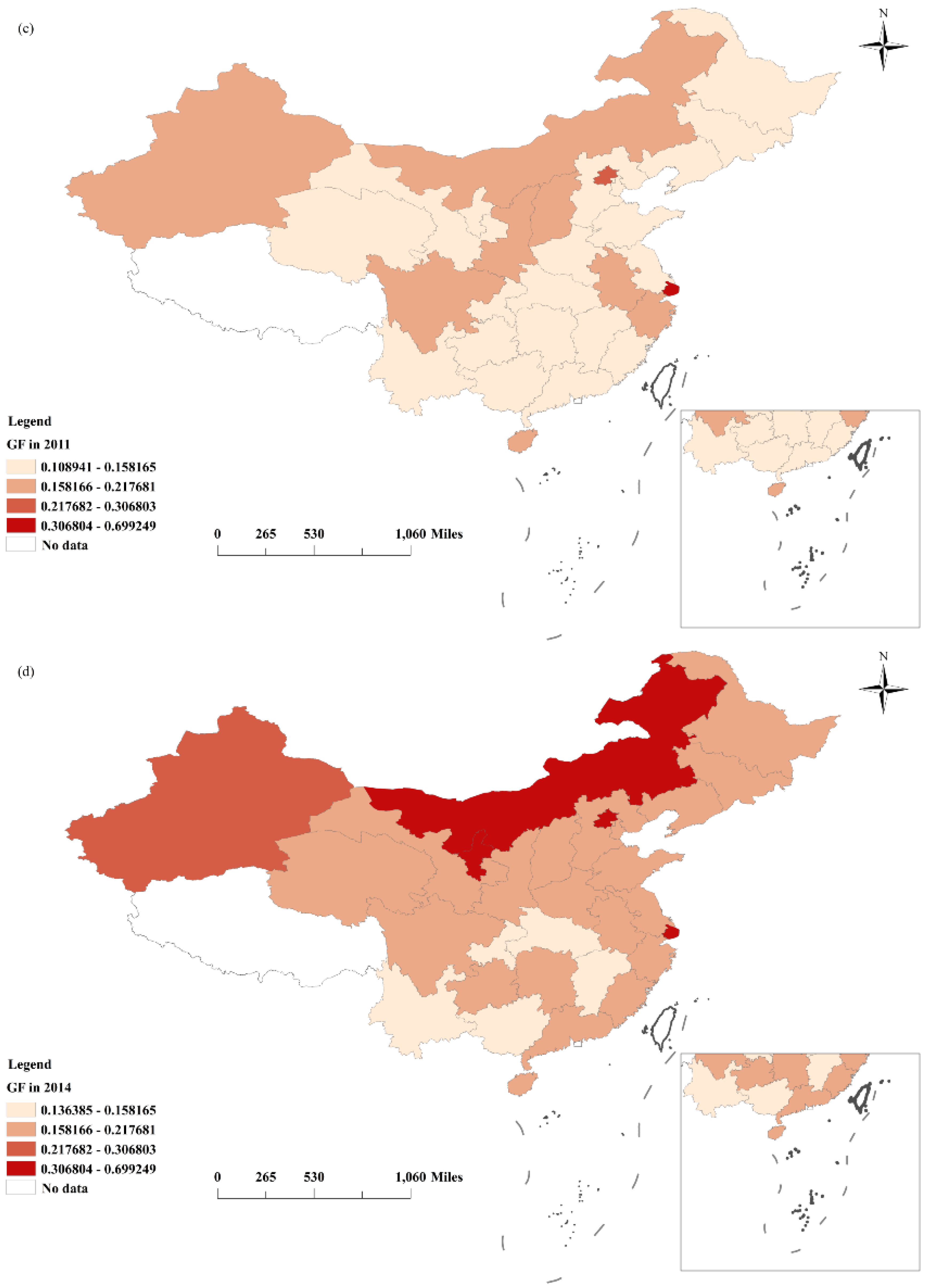
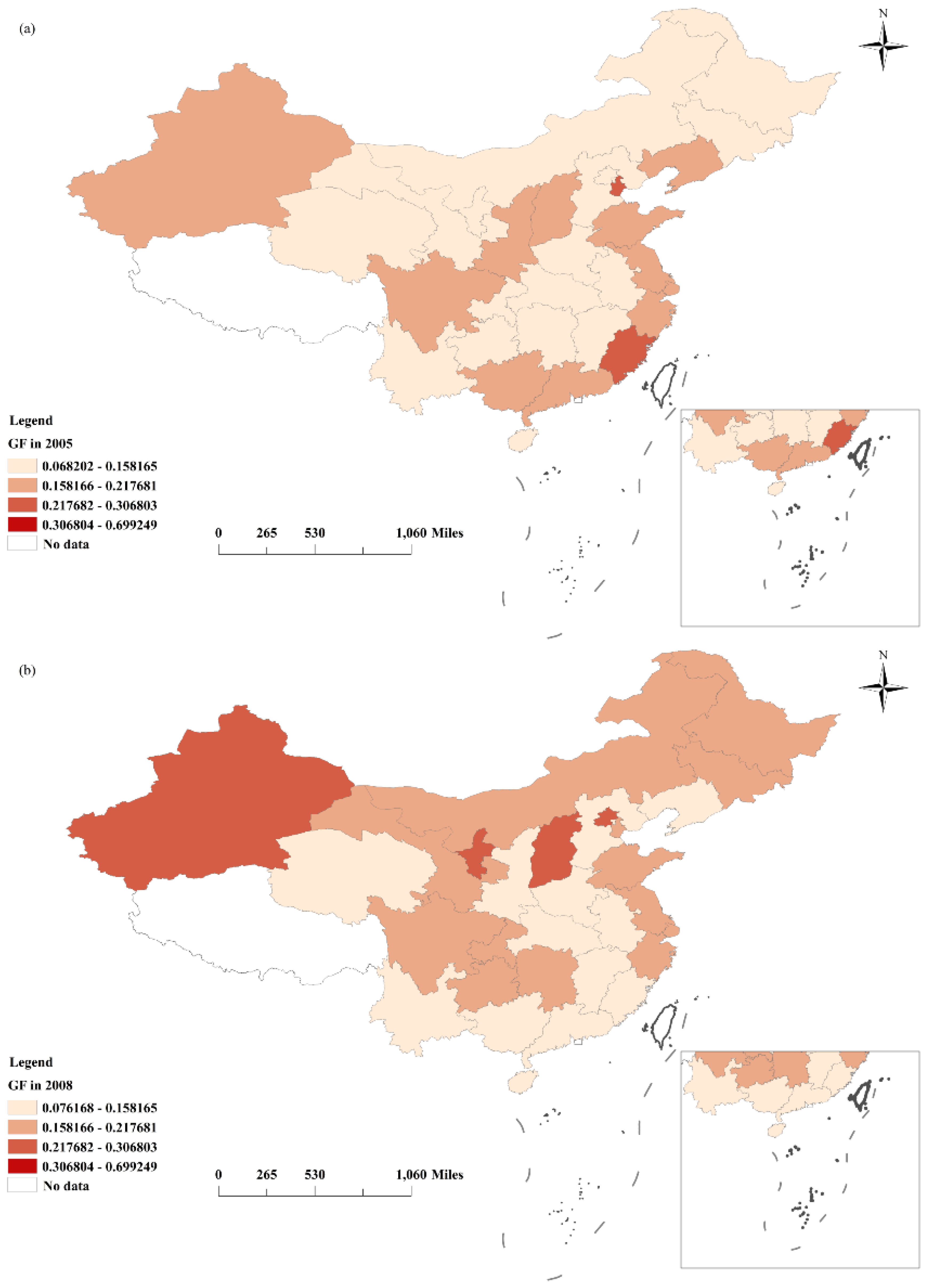
According to Equations (12)–(16), the weights of the secondary indicators for measuring GF in Table 1 were 0.564, 0.288, 0.080, 0.037, and 0.031. The results of the GF calculations are shown in Figure 2. During the study period, GF showed an overall improvement trend. However, the values of GF are almost below 0.699; therefore, significant improvement is still needed.

4.1.2. IEE Calculation Results

Figure 3 illustrates the regional average values of IEE. Compared with the IEE in the western region, the IEE in the eastern region is greater than in the central region, and the southwestern region is greater than in the northwestern region. This may be due to the differences in resource endowments, and economic and social development levels in different regions.

4.2. Empirical Results

4.2.1. Benchmark Regression Results

The average variance inflation factor (VIF) was 4.05, i.e., less than 5 (see Table 4). Hence, there was no significant multi-collinearity among the selected variables.
To estimate GF’s impact on IEE, we referred to Lee and Wang [23] and used the ordinary least square (OLS) method to test Equation (1). Table 5 shows the results. Column (2) illustrates the results without control variables under year fixed and provincial fixed effects. Columns (3)–(6) present the results of GF on IEE after gradually incorporating the control variables under the two-way fixed effects. The results are more robust after incorporating the year fixed and provincial fixed effects, and the control variables, which are interpreted in Column (6). The coefficient value in Column (6) is 7.338 at a significance level of 1%, which suggests that GF positively affects IEE. Thus, Hypothesis 1 is verified. Our results are consistent with those of Guo et al. [20], but the reverse of those of Wang et al. [27], who concluded that GF could not improve energy efficiency nationally [27]. The possible reasons are the differences between the research subjects, control variable selections, and variable processing methods.
Column (6) also shows that FDI, GDP, EL, and TI significantly contribute to the improvement of IEE. However, UR, ECS, and ER significantly negatively affect IEE. This can be explained by the large amount of redundant infrastructure construction in China’s urbanization process, which leads to a significant waste of resources. In addition, the high proportion of coal consumption in primary energy consumption and overly strict environmental regulations are also not conducive to enhancing IEE.

4.2.2. Robustness Tests

For the robustness tests, we lagged the GF for one period, replaced the explanatory variable, and replaced the model with a fixed effect (FE) [51] and dynamic panel model (see Table 6) [54]. These results are consistent with the benchmark regression. Hence, the results are robust.

4.2.3. Moderating Effect Regression Results

We estimated Equations (3) and (4) to test the moderating effects of the marketization level (ML), and Table 7 displays the outcomes. Column (2) and Column (3) show the calculation results of the main effect and moderation effect models, respectively. Column (2) indicates that GF significantly promotes IEE improvement. As shown in Column (3), the interaction term coefficient is 1.426 at the 1% significance level, indicating that ML favorably modifies the improving effect of GF on IEE. Column (4) shows the test results after decentralization, and illustrates that the interaction term coefficient is also positive, thus indicating that ML strengthens GF’s impact on IEE again. As a result, Hypothesis 2 is confirmed.

4.2.4. Threshold Effect Regression Results

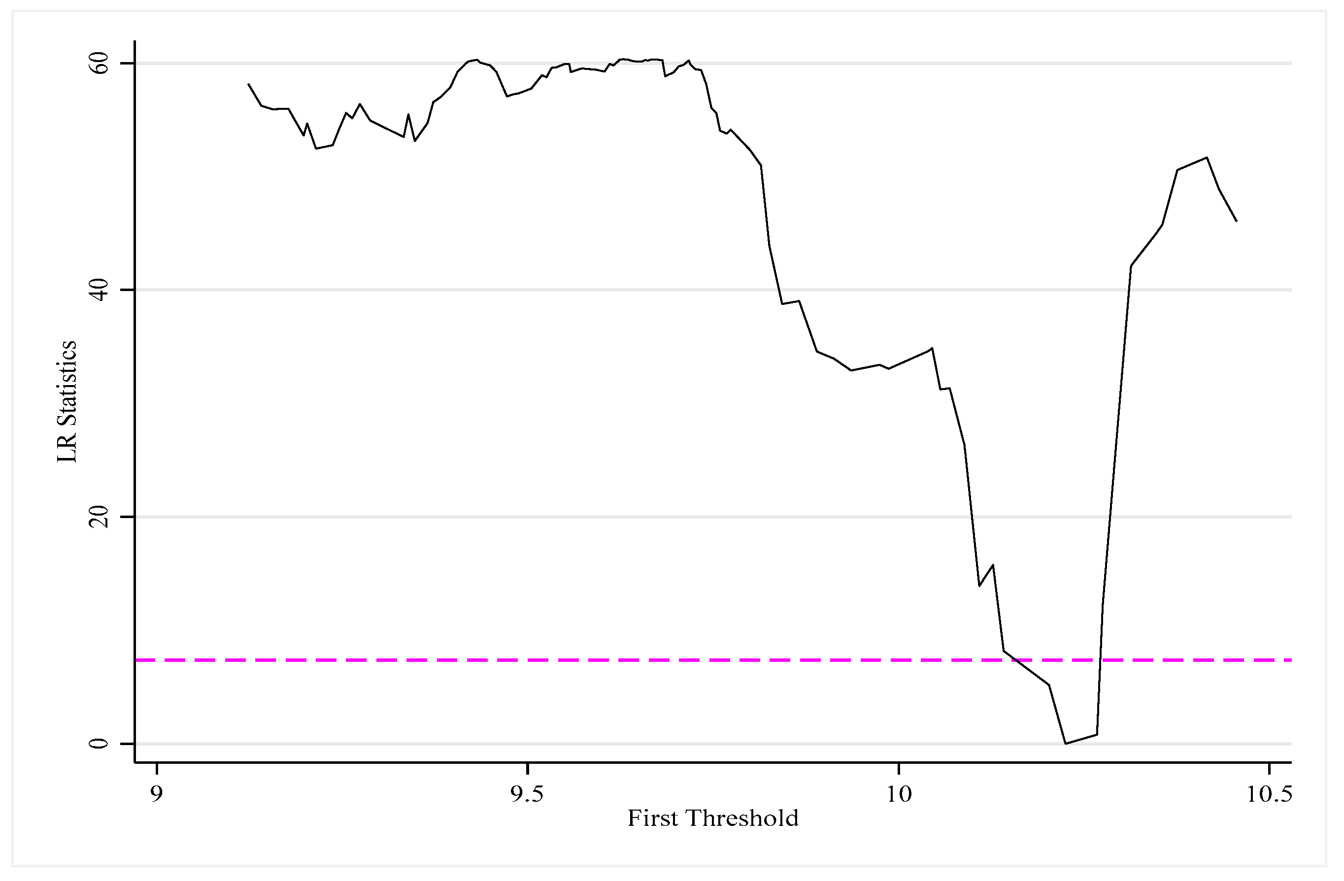
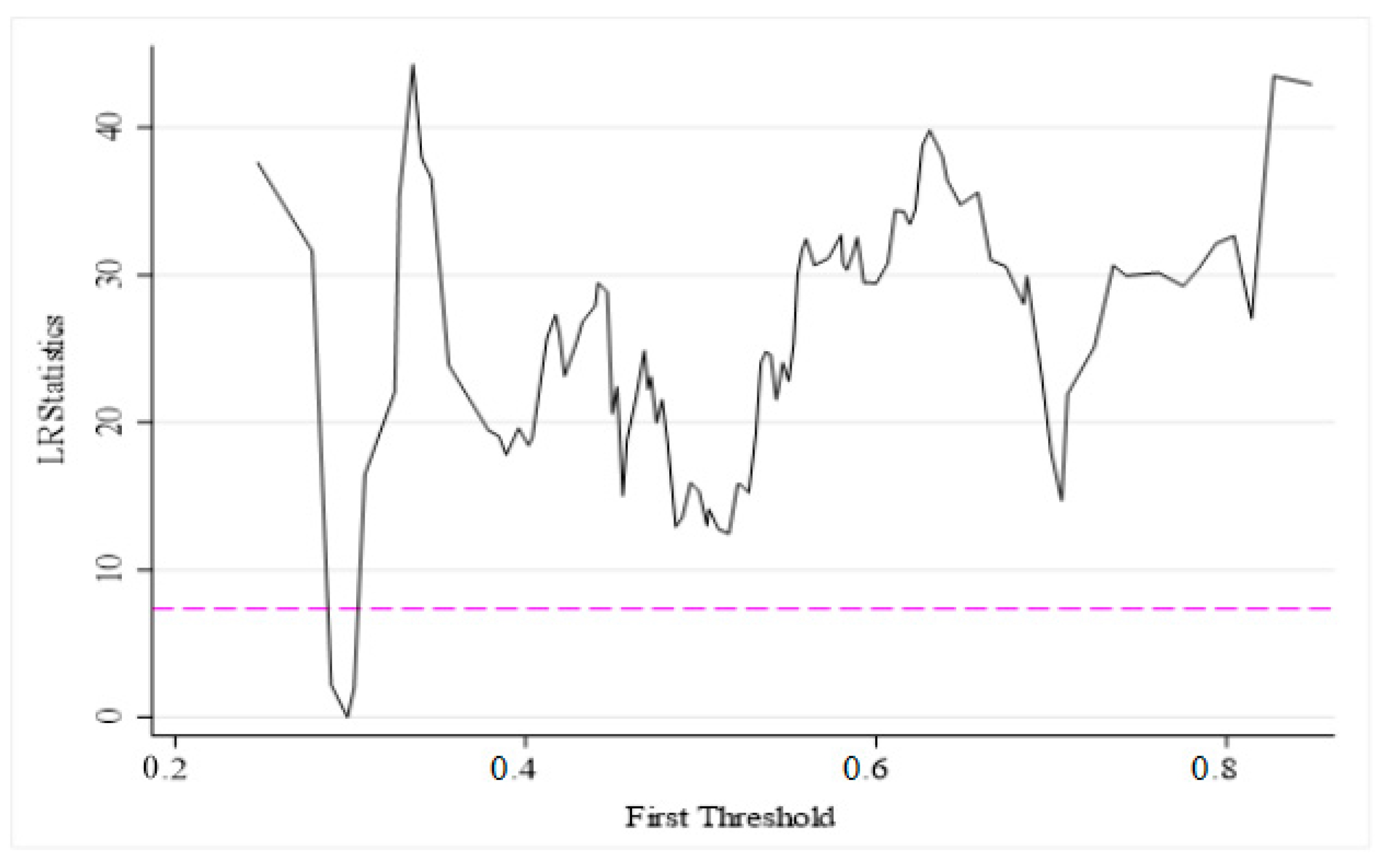
Stata17.0 software was used and sampling was repeated 500 times, using the self-service method based on Equation (5), to verify the nonlinear impact of GF on IEE. When EDL and GCL were used as threshold variables, it can be observed that neither passed the double and triple threshold tests; they belong to single threshold effects. Table 8 and Figure 4 show the results when economic development (EDL) is the threshold variable with a truncated tail of 0.05. When EDL is ≤10.225, for every 1% increase in GF, the IEE increases by 1.783%. When the EDL is >10.225, for every 1% increase in GF, the IEE increases by 16.319%. When the EDL exceeds the threshold, GF’s impact on IEE gradually increases. A main reason for this is that, in the regions with higher EDL, the funds used for industrial green development are sufficient, which is more conducive to improving IEE. Table 9 and Figure 5 report the results when green credit (GCL) is used as a threshold variable. When GCL is ≤0.298, for every 1% increase in GF on average, IEE increases by 12.649%. When GCL is >0.298, for every 1% increase in GF on average, IEE increases by 5.378%. That is, when GCL exceeds the threshold, although the impact of GF on IEE is somewhat weakened, it still shows a promoting effect. In areas where GCL is relatively weak, the GF is more sensitive to the growth of green investment and technological innovation and has a more substantial promoting effect on IEE. However, with increases in GCL, the differences in industrial structure and technical levels between regions will decrease, and the promoting effect of GF on IEE will weaken. In summary, Hypothesis 3 holds.

4.2.5. Heterogeneity Test

As shown in Table 10, GF significantly improves IEE in the central and eastern areas and has a negative effect in the western area. These results can be explained by the fact that industry in the eastern area has shifted to the central region, a significant shift that should be supported and allowed to play more of a spillover effect. The results of the western region are similar to those of Wang and Wang [27]. One possible reason is that the response of some industrial enterprises to government emission requirements in the western area is only to effect reductions in production efficiency as much as possible, due to a lack of funding support. Table 10 also reports that the GF in the northwestern and southwestern areas negatively affects IEE but is insignificant.

4.3. Results of Spatial Effect Model

4.3.1. Results of the Spatial Clustering Characteristics of IEE

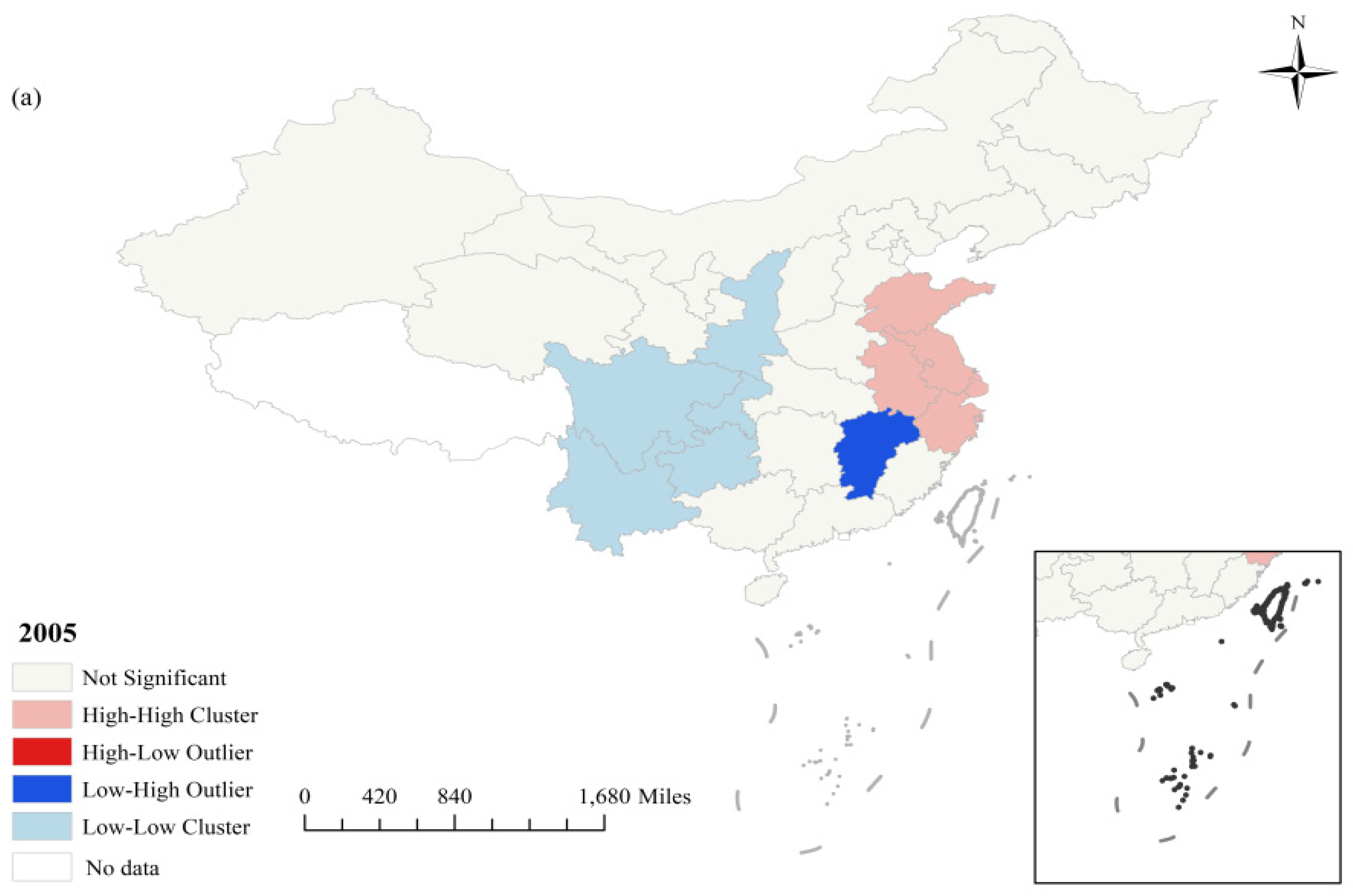
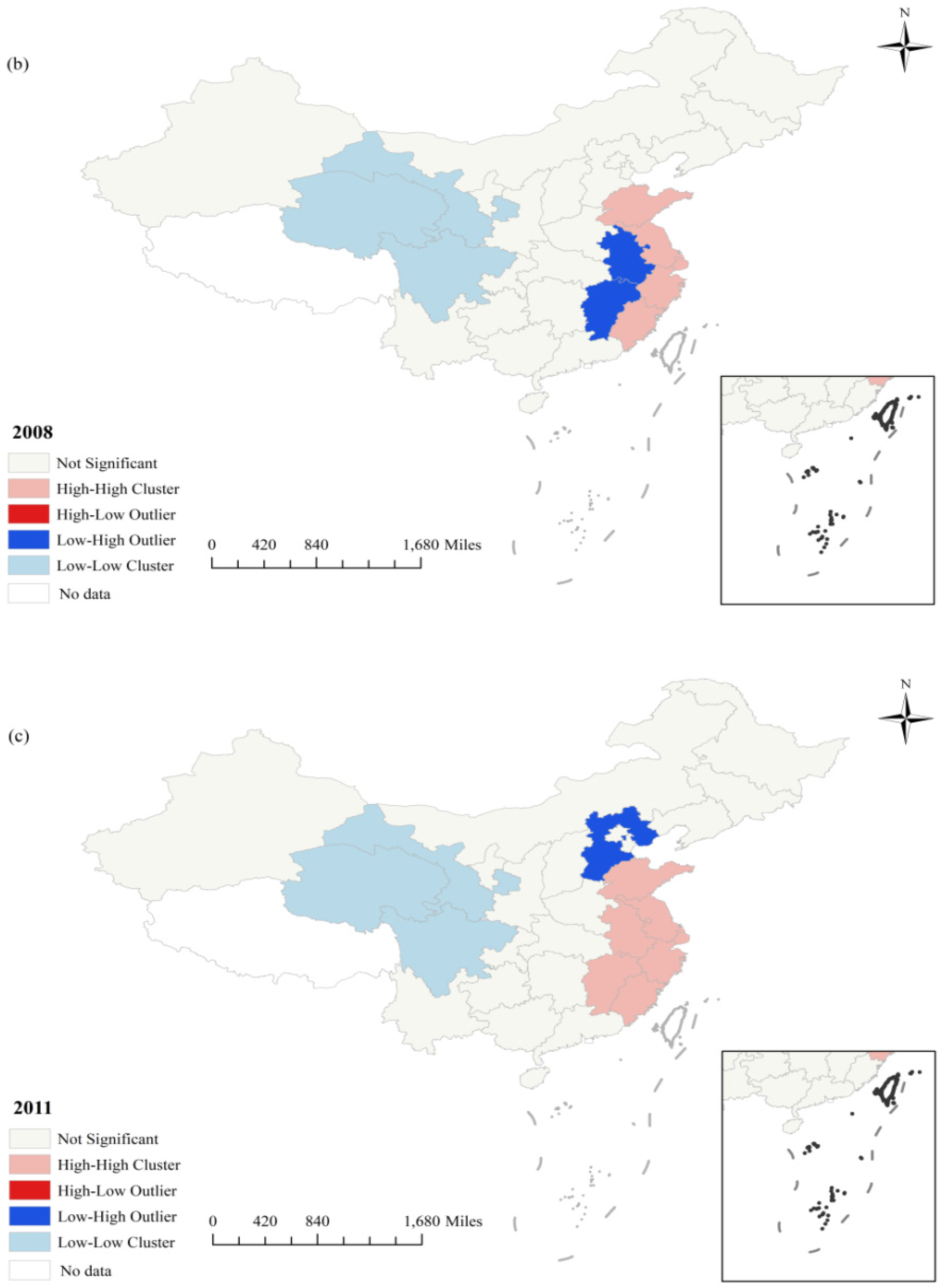
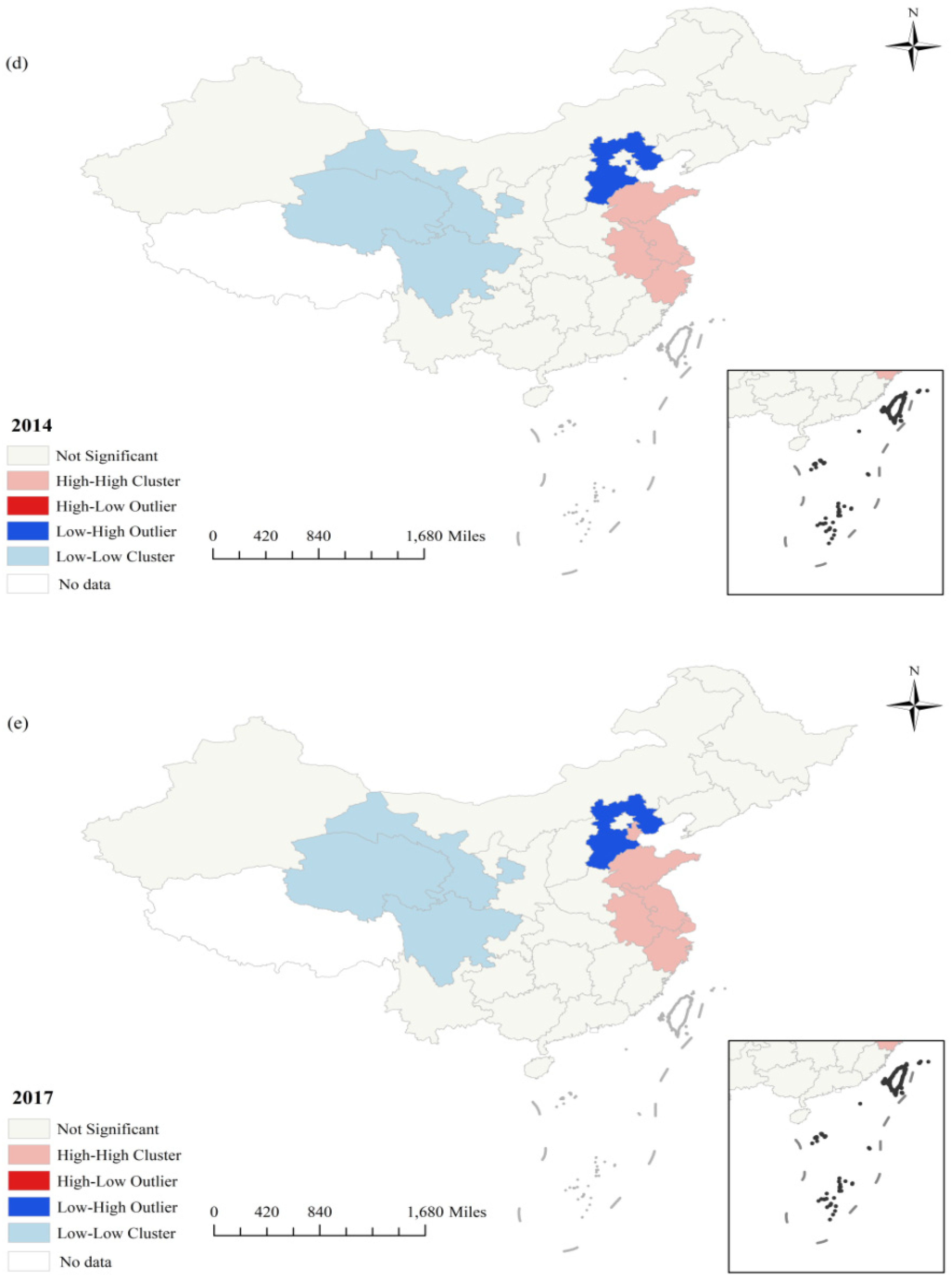
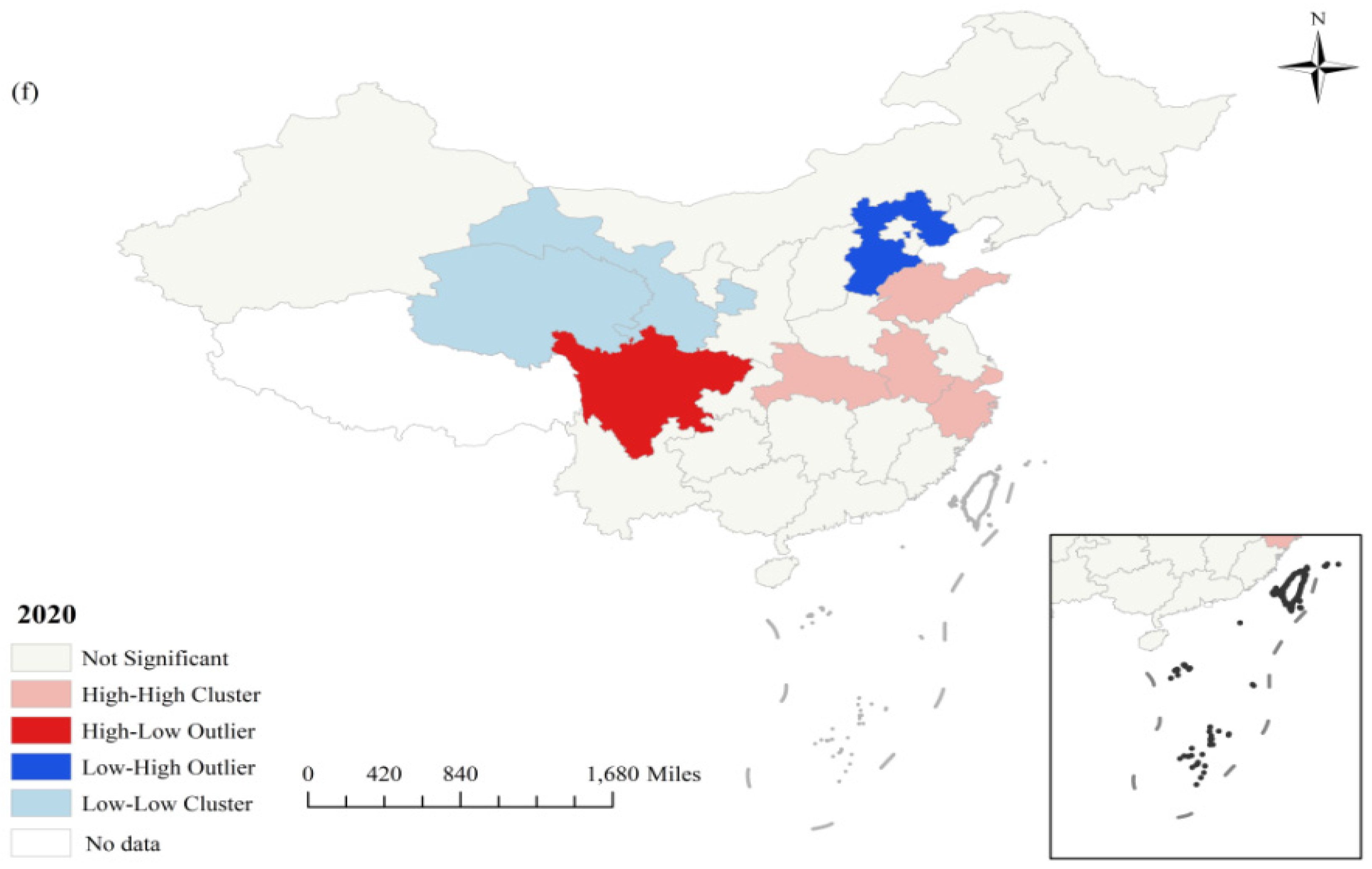
We divided the study period into six periods to dynamically display the spatial autocorrelation features of IEE that change over time every three years. We used ArcGIS 10.8 software to display the divisions of IEE in the provinces at the end of each period on the map according to Equation (6). Figure 6 shows that the Anselin Local Moran’s I shows four types of clusters, and Yu et al. [45] provided a detailed explanation of those clusters. The IEE in most provinces can be observed as showing similar spatial clustering characteristics. The high–high clustering provinces are located in the eastern and central areas, and the levels of IEE of these provinces and their surrounding areas are high [40]. The low–high provinces are also located in central and east areas, and the IEE levels of these provinces are low; meanwhile, their surrounding provinces show high levels. This is because most provinces in the eastern and central regions have advanced technology, equipment, and high-quality skills in the working population. The low–low and high–low clustering provinces are located in the western area. The possible reason is that these provinces have low levels of technological development, inconvenient transportation routes, and traditional resource-based industrial structures. Moreover, only about one-third of the provinces show the significant spatial clustering characteristics of IEE, which indicates that the radiation effects of the high IEE provinces have a less significant beneficial influence on adjacent provinces [45].

4.3.2. Analysis of Spatial Spillover Effects

We employed the LM test to investigate the types of spatial correlation influencing how GF affects IEE. The p -value for the SEM’s LM is 0.15 and greater than 0.1, which is not significant. The LM’s p -value for the SLM is 0.084 and less than 0.1, which is significant. Therefore, an SLM, i.e., Equation (7), needs to be used for the subsequent analysis. Meanwhile, the Hausman test determines whether the SLM adopts either fixed or random effects. Because the Hausman test’s c h i 2 9 = b B V b V B 1 b B = 39.24 > 0 ,   P r o b > c h i 2 = 0.0000 < 0.1 is significant, a fixed effect model was used. Moreover, the fixed effects can be further categorized into time fixed, individual fixed, and two-way fixed effects. Therefore, the likelihood ratio (LR) test needs to be used to determine which fixed effect is more suitable for the model constructed. When the null hypothesis, H0, is compared between the two-way fixed and individual fixed effects, L R   c h i 2 11 = 49.46 ,   P r o b > c h i 2 = 0.0000 are obtained. When comparing the time fixed and two-way fixed effects under the null hypothesis, H0, L R   c h i 2 11 = 408.77 ,   P r o b > c h i 2 = 0.0000 are obtained. Therefore, we adopted the two-way fixed effects of SLM.
For a more specific analysis of the impact of GF on IEE, with reference to LeSage and Pace [55], the various effects of GF on IEE are captured through regressing the two-way fixed effects of SLM, as shown in Table 11. Column (2) reveals that GF can provide a positive spatial spillover effect to IEE in the local area, which is similar to Guo et al. [20]. This is because GF provides sufficient funding for green projects in local industrial enterprises while forcing traditional industrial enterprises to accelerate transition and upgrading, then promoting the improvement of IEE in the local area. Column (3) demonstrates that the indirect effect of GF on IEE is −1.476 at the 5% significance level; therefore, GF has a negative spatial spillover effect on IEE in neighboring areas. It can be explained with the phenomenon of the siphonic effect [27]. Therefore, Hypothesis 4 is verified. Column (4) shows that the total effect of GF on IEE is 6.004.

5. Discussion

In this section, we discuss several policy recommendations and illustrate how our results will affect further research.
First, more policies should be instituted so that GF can effectively improve IEE. The previous research has revealed that the most significant obstacle to energy efficiency improvement is insufficient investment; therefore, the limitations of green financing and renewable energy policies must be addressed [8]. The GF system of China is still in its initial stages; consequently, more policy support should be provided [9]. Specifically, the policymakers should introduce policies that encourage banking institutions to innovate and develop diversified and flexible GF portfolio products. For example, measures such as relaxing loan conditions, lowering interest rates, and providing longer loan terms and flexible repayment methods should be put in place to guarantee that industrial green and low-carbon transition projects have sufficient funding support [13]. Moreover, the local government must deliver policy documents to encourage industrial enterprises to increase their annual R&D expenditure. For instance, cooperation between government, industry, and the academic community should be strengthened [5] to solve those bottleneck problems that industrial enterprises face through the performance of significant scientific research projects. In addition, policymakers should formulate and revise differentiated GF and energy-efficiency improvement policies based on the actual industrial situation, and the corresponding supporting mechanisms should be provided to maximize policy implementation effectiveness.
Second, it is crucial to increase the marketization level. Our results suggest that ML significantly positively regulates the promotional effect of GF on IEE. Therefore, the government should accelerate the market-oriented reform based on the regional marketization process. For example, government interventions in resource allocation should gradually be reduced. Additionally, the institutional barriers should be eliminated, and competition mechanisms should be introduced, creating a favorable market environment for the development of various industries. In addition, market-oriented mechanisms should be fully employed to stimulate green innovation in state-owned and private enterprises and to improve their overall competitiveness. For example, economic incentive policies should be prepared to encourage industrial enterprises to develop green and highly efficient equipment and processes [7], helping to obtain GF support to improve IEE.
Third, it is critical to improve the level of GF. Our results indicate that GF’s impact on IEE exhibits a single threshold effect of EDL and GCL. China‘s economic growth rate has declined. Zhou et al. [8] found that GF can significantly improve economic development; therefore, improving the level of GF is crucial. However, GF is still in its early stages and so the GF levels in various provinces must be accelerated for improvement. A key responsibility of the provincial governments is to define clearly the scope of GF’s project support and payment standards, thereby helping to ensure that GF is used effectively. Moreover, the provincial statistical departments should strive to perform excellent annual statistical monitoring related to GF, such as identifying which projects in the industrial sector receive GF investment every year and accurately calculating the total investment amount. In addition, a tracking mechanism should be established to conduct the post-evaluation of the invested projects, the timely disclosure of the effectiveness of GF-supported projects, and the further optimization and adjustment of GF’s relevant policy design. Moreover, the government should accelerate the establishment of provincial and regional integrated GF service platforms, strengthen deep cooperation among banks, insurance companies, professional institutions, and leading enterprises in the green industry, and improve GF levels in various provinces.
Last, it is critical to encourage cooperation and exchanges between industrial enterprises. Specifically, the industrial enterprises in the western area could accelerate the transition and perform upgrades through learning from the advanced experiences of the eastern and central areas. The central area should play a bridging role, and the eastern region could obtain rewards by providing guidance services for industrial enterprises in the western and central regions, achieving win–win development. Moreover, strengthening the cooperation of industrial enterprises within the same region [56] would promote the overall regional improvements in IEE. In addition, the local government should eliminate regional barriers, further accelerate the free flow of elements, and optimize the resource allocation between regions [40].
The results of this study will influence future research through the following aspects:
(1) Our study has strengthened the determination of the Chinese government and enterprises to enhance IEE by leveraging GF. Researchers should increase their research on the optimization design of policy systems for GF and energy efficiency improvement, and conduct simulation of policy effects to help the government revise general and differentiated policy documents. (2) Scholars should strengthen the exploration of achieving market-oriented operation mechanisms in the industrial sector and help GF improve its role in improving IEE. (3) Scholars need to increase research on improving or reconstructing traditional economic growth models and find long-term stable economic growth conditions and paths in the digital economy era. At the same time, they should increase research on the theoretical models of how GF can effectively support industrial green and low-carbon transformation. (4) The government should enhance research on communication and cooperation mechanisms among industrial enterprises in different regions of China and achieve win–win development for industrial enterprises.

6. Conclusions

In this study, GF’s impact on IEE was analyzed. Accordingly, GF and IEE were measured using the entropy method and the reciprocal of industrial energy intensity based on the 2005–2020 panel data of 30 of China’s provinces. On this basis, we adopted a two-way fixed effects model to study GF’s impact and regional heterogeneity on IEE. The various effects of GF on IEE were examined. The spatial autocorrelation of IEE was also analyzed. The main conclusions are set out below.
(1)
In China, improving IEE through GF is feasible. GF can significantly and positively promote IEE but exhibits significant regional heterogeneity. After incorporating the year fixed and provincial fixed effects and the control variables, the benchmark regression results indicate that every 1% increase in GF leads to a 7.338% increase in IEE at a significance level of 1%. The finding is consistent even after extensive testing for robustness. GF significantly positively improved the IEE in the central and eastern areas and negatively affected IEE in the western area.
(2)
Increasing the marketization level will help GF further improve IEE. After decentralization, the interaction term coefficient is 1.426 at a significance level of 1%, indicating that ML significantly positively regulates the promotional effect of GF on IEE.
(3)
Enhancing the level of GF is important. GF’s impact on IEE exhibits single threshold effects of EDL and GCL. When EDL exceeds the threshold, the GF’s impact on IEE gradually increases. When GCL exceeds the threshold, although the impact of GF on IEE is somewhat weakened, it still shows a promoting effect.
(4)
Strengthening exchanges and cooperation between different industrial enterprises is essential. The IEE shows four types of clusters, such as high–high, high–low, low–high, and low–low clusters, but only about one-third of the provinces show the significant spatial clustering characteristics of IEE. The direct and indirect effects of GF on IEE are 7.479 and −1.476 at the 1% and 5% significance levels, indicating that GF can promote local IEE improvement but prevent neighboring IEE improvement.
(5)
Strengthening policy support is necessary. For example, introduce policies encouraging banking institutions to innovate and develop diversified and flexible GF portfolio products, encourage industrial enterprises to increase annual R&D expenditure, and formulate and revise differentiated GF and energy-efficiency improvement policies.
This study investigates the various impacts of GF on China’s IEE. Further research and comparative analyses should be conducted on the relationship between GF and IEE in different countries or regions. In addition, when formulating the hypothesis, we did not propose the research proposition by constructing a mathematical model but instead proposed it through textual explanation. Later, we need to establish a mathematical model of GF influencing IEE to derive the research proposition and empirically test the research hypothesis. In fact, GF mainly promotes IEE improvement by funding support for green projects, thereby helping achieve industrial green and low-carbon transformation and development. However, there is no statistical disclosure in China regarding which green projects GF has invested in within the industrial sector and how much it has invested in these projects. Therefore, this study did not obtain this information. Although we empirically tested the various effects of GF on IEE at the industrial level based on existing statistical data, supplementing previous research that focused on analyzing the impact of GF on energy efficiency at a macro level, further research is still needed. Specifically, more micro-level research on industrial enterprises is required. By conducting on-site research on multiple banking institutions, one can obtain first-hand information on which projects GF has mainly invested in and how much it has invested in these projects, and then empirically test GF’s impact on energy efficiency in industrial enterprises. Moreover, mediation effect analysis at the industrial enterprises level can also be included.

Author Contributions

Proposal of the original idea, conception, and review of the paper, J.Z.; writing and editing of the paper, L.C. All authors have read and agreed to the published version of the manuscript.

Funding

This study was funded by the National Natural Science Foundation of China (71273206).

Data Availability Statement

Data will be made available on request.

Conflicts of Interest

The authors declare no conflict of interest.

References

  1. Wang, B. Low-Carbon Transformation Planning of China’s Power Energy System under the Goal of Carbon Neutrality. Environ. Sci. Pollut. Res. 2023, 30, 44367–44377. [Google Scholar] [CrossRef] [PubMed]
  2. Zhang, X.; Huang, X.; Zhang, D.; Geng, Y.; Tian, L.; Fan, Y.; Chen, W. Research on the Pathway and Policies for China’s Energy and Economy Transformation toward Carbon Neutrality. J. Manag. World 2022, 38, 35–66. [Google Scholar] [CrossRef]
  3. Yu, M.; Zhou, Q.; Cheok, M.Y.; Kubiczek, J.; Iqbal, N. Does Green Finance Improve Energy Efficiency? New Evidence from Developing and Developed Economies. Econ. Chang. Restruct. 2022, 55, 485–509. [Google Scholar] [CrossRef]
  4. Pérez-Lombard, L.; Ortiz, J.; Velázquez, D. Revisiting Energy Efficiency Fundamentals. Energy Effic. 2013, 6, 239–254. [Google Scholar] [CrossRef]
  5. Cai, L.; Song, X.; Zhang, J.; Xing, Y. Post-Evaluation Analysis on Urban Coal, Oil and Gas Resources Comprehensive Utilization Governance Project: A Case Study in Fuxian, China. Heliyon 2023, 9, e16732. [Google Scholar] [CrossRef] [PubMed]
  6. National Bureau of Statistics of the People’s Republic of China. China Statistical Yearbook 2023; National Bureau of Statistics of the People’s Republic of China: Beijing, China, 2023.
  7. Song, X.; Geng, Y.; Li, K.; Zhang, X.; Wu, F.; Pan, H.; Zhang, Y. Does Environmental Infrastructure Investment Contribute to Emissions Reduction? A Case of China. Front. Energy 2020, 14, 57–70. [Google Scholar] [CrossRef]
  8. Zhou, X.; Tang, X.; Zhang, R. Impact of Green Finance on Economic Development and Environmental Quality: A Study Based on Provincial Panel Data from China. Environ. Sci. Pollut. Res. 2020, 27, 19915–19932. [Google Scholar] [CrossRef]
  9. Du, J.; Shen, Z.; Song, M.; Vardanyan, M. The Role of Green Financing in Facilitating Renewable Energy Transition in China: Perspectives from Energy Governance, Environmental Regulation, and Market Reforms. Energy Econ. 2023, 120, 106595. [Google Scholar] [CrossRef]
  10. Wang, X.; Wang, Q. Research on the Impact of Green Finance on the Upgrading of China’s Regional Industrial Structure from the Perspective of Sustainable Development. Resour. Policy 2021, 74, 102436. [Google Scholar] [CrossRef]
  11. Yang, Y.; Su, X.; Yao, S. Nexus between Green Finance, Fintech, and High-Quality Economic Development: Empirical Evidence from China. Resour. Policy 2021, 74, 102445. [Google Scholar] [CrossRef]
  12. Chen, J.; Abbas, J.; Najam, H.; Liu, J.; Abbas, J. Green Technological Innovation, Green Finance, and Financial Development and Their Role in Green Total Factor Productivity: Empirical Insights from China. J. Clean. Prod. 2023, 382, 135131. [Google Scholar] [CrossRef]
  13. Song, X.; Geng, Y.; Dong, H.; Chen, W. Social Network Analysis on Industrial Symbiosis: A Case of Gujiao Eco-Industrial Park. J. Clean. Prod. J. 2018, 193, 414–423. [Google Scholar] [CrossRef]
  14. Azhgaliyeva, D.; Kapoor, A.; Liu, Y. Green Bonds for Financing Renewable Energy and Energy Efficiency in South-East Asia: A Review of Policies. J. Sustain. Financ. Investig. 2020, 10, 113–140. [Google Scholar] [CrossRef]
  15. Xiong, Y.; Dai, L. Does Green Finance Investment Impact on Sustainable Development: Role of Technological Innovation and Renewable Energy. Renew. Energy 2023, 214, 342–349. [Google Scholar] [CrossRef]
  16. Wan, Y.; Sheng, N.; Wei, X.; Su, H. Study on the Spatial Spillover Effect and Path Mechanism of Green Finance Development on China’s Energy Structure Transformation. J. Clean. Prod. 2023, 415, 137820. [Google Scholar] [CrossRef]
  17. Zhang, H.; Duan, Y.; Yang, J.; Han, Z.; Wang, H. Can Green Finance Improve China’s Haze Pollution Reduction? The Role of Energy Efficiency. Environ. Dev. 2023, 45, 100833. [Google Scholar] [CrossRef]
  18. Kong, Z.; Lu, X.; Dong, X.; Jiang, Q.; Elbot, N. Re-Evaluation of Energy Return on Investment (EROI) for China’s Natural Gas Imports Using an Integrative Approach. Energy Strategy Rev. 2018, 22, 179–187. [Google Scholar] [CrossRef]
  19. Wei, Y.; Liao, H. Seven Types of Energy Efficiency Measurement Indicators and Their Measurement Methods. China Soft Sci. 2010, 1, 128–137. [Google Scholar]
  20. Guo, Q.T.; Dong, Y.; Feng, B.; Zhang, H. Can Green Finance Development Promote Total-Factor Energy Efficiency? Empirical Evidence from China Based on a Spatial Durbin Model. Energy Policy 2023, 177, 113523. [Google Scholar] [CrossRef]
  21. Hu, Y.; Hall, C.A.S.; Wang, J.; Feng, L.; Poisson, A. Energy Return on Investment (EROI) of China’s Conventional Fossil Fuels: Historical and Future Trends. Energy 2013, 54, 352–364. [Google Scholar] [CrossRef]
  22. Lee, C.; Lee, C. How Does Green Finance Affect Green Total Factor Productivity? Evidence from China. Energy Econ. 2022, 107, 105863. [Google Scholar] [CrossRef]
  23. Lee, C.C.; Wang, C.S.; He, Z.; Xing, W.W.; Wang, K. How Does Green Finance Affect Energy Efficiency? The Role of Green Technology Innovation and Energy Structure. Renew. Energy 2023, 219, 119417. [Google Scholar] [CrossRef]
  24. Xu, K.; Zhao, P. Does Green Finance Promote Green Total Factor Productivity? Empirical Evidence from China. Sustainability 2023, 15, 11204. [Google Scholar] [CrossRef]
  25. Tan, X.; Xiao, Z.; Liu, Y.; Taghizadeh-Hesary, F.; Wang, B.; Dong, H. The Effect of Green Credit Policy on Energy Efficiency: Evidence from China. Technol. Forecast. Soc. Chang. 2022, 183, 121924. [Google Scholar] [CrossRef]
  26. Liu, H.; Yao, P.; Latif, S.; Aslam, S.; Iqbal, N. Impact of Green Financing, FinTech, and Financial Inclusion on Energy Efficiency. Environ. Sci. Pollut. Res. 2022, 29, 18955–18966. [Google Scholar] [CrossRef]
  27. Wang, Z.; Wang, X. Research on the Impact of Green Finance on Energy Efficiency in Different Regions of China Based on the DEA-Tobit Model. Resour. Policy 2022, 77, 102695. [Google Scholar] [CrossRef]
  28. Hou, Y.; Li, X.; Wang, H.; Yunusova, R. Focusing on Energy Efficiency: The Convergence of Green Financing, FinTech, Financial Inclusion, and Natural Resource Rents for a Greener Asia. Resour. Policy 2024, 93, 105052. [Google Scholar] [CrossRef]
  29. Meng, Y.; Liu, L.; Ran, Q. Does Green Finance Improve Energy Efficiency?—Based on a Chinese Government R&D Subsidy Perspective. Ecol. Econ. 2018, 39, 45–53. [Google Scholar]
  30. Ge, T.; Cai, X.; Song, X. How Does Renewable Energy Technology Innovation Affect the Upgrading of Industrial Structure? The Moderating Effect of Green Finance. Renew. Energy 2022, 197, 1106–1114. [Google Scholar] [CrossRef]
  31. Huo, D.; Zhang, X.; Meng, S.; Wu, G.; Li, J.; Di, R. Green Finance and Energy Efficiency: Dynamic Study of the Spatial Externality of Institutional Support in a Digital Economy by Using Hidden Markov Chain. Energy Econ. 2022, 116, 106431. [Google Scholar] [CrossRef]
  32. Song, X.; Mu, X. The Safety Regulation of Small-Scale Coal Mines in China: Analysing the Interests and Influences of Stakeholders. Energy Policy 2013, 52, 472–481. [Google Scholar] [CrossRef]
  33. Zhang, M.; Di, Q.; Feng, T. Heterogeneous R&D and “Productivity Dilemma”: The Moderating Effect of Government Support and Marketization. Soft Sci. 2023, 38, 61–69. 1–14. [Google Scholar]
  34. Ma, Q.; Liu, X.; Wang, W.G.; Xue, J. Natural Resources Extraction and COP26 Target: Evaluating the Role of Green Finance. Resour. Policy 2023, 82, 103432. [Google Scholar] [CrossRef]
  35. Yin, X.; Chen, D.; Ji, J. How Does Environmental Regulation Influence Green Technological Innovation? Moderating Effect of Green Finance. J. Environ. Manag. 2023, 342, 118112. [Google Scholar] [CrossRef]
  36. Lan, J.; Wei, Y.; Guo, J.; Li, Q.; Liu, Z. The Effect of Green Finance on Industrial Pollution Emissions: Evidence from China. Resour. Policy 2023, 80, 103156. [Google Scholar] [CrossRef]
  37. Xu, J.; Li, J.; Nie, D.; Shen, X. To Green or to Work: The Labor Demand Reduction Effect of Green Finance. Environ. Sci. Pollut. Res. 2023, 30, 63899–63914. [Google Scholar] [CrossRef]
  38. Li, R.; Liu, Q.; Cai, W.; Liu, Y.; Yu, Y.; Zhang, Y. Echelon Peaking Path of China’s Provincial Building Carbon Emissions: Considering Peak and Time Constraints. Energy 2023, 271, 127003. [Google Scholar] [CrossRef]
  39. Wang, F.; Wang, R.; He, Z. The Impact of Environmental Pollution and Green Finance on the High-Quality Development of Energy Based on Spatial Dubin Model. Resour. Policy 2021, 74, 102451. [Google Scholar] [CrossRef]
  40. Wang, Z.; Sun, Y.; Yuan, Z.; Wang, B. Does Energy Efficiency Have a Spatial Spill-over Effect in China? Evidence from Provincial-Level Data. J. Clean. Prod. 2020, 241, 118258. [Google Scholar] [CrossRef]
  41. Zhou, X.; Tang, X. Spatiotemporal Consistency Effect of Green Finance on Pollution Emissions and Its Geographic Attenuation Process. J. Environ. Manag. 2022, 318, 115537. [Google Scholar] [CrossRef]
  42. Wu, K.; You, K.; Ren, H.; Gan, L. The Impact of Industrial Agglomeration on Ecological Efficiency: An Empirical Analysis Based on 244 Chinese Cities. Environ. Impact Assess. Rev. 2022, 96, 106841. [Google Scholar] [CrossRef]
  43. Baron, R.M.; Kenny, D.A. The Moderator-Mediator Variable Distinction in Social Psychological Research: Conceptual, Strategic, and Statistical Considerations. J. Pers. Soc. Psychol. 1986, 51, 1173–1182. [Google Scholar] [CrossRef] [PubMed]
  44. Wang, N.; Zhu, Y.; Yang, T. The Impact of Transportation Infrastructure and Industrial Agglomeration on Energy Efficiency: Evidence from China’s Industrial Sectors. J. Clean. Prod. 2020, 244, 118708. [Google Scholar] [CrossRef]
  45. Yu, Z.; Guo, T.; Song, X.; Zhang, L.; Cai, L.; Zhang, X.; Zhao, A. Green Transition Assessment, Spatial Correlation, and Obstacles. Land 2024, 13, 341. [Google Scholar] [CrossRef]
  46. Liu, R.; Wang, D.; Zhang, L.; Zhang, L. Can Green Financial Development Promote Regional Ecological Efficiency? A Case Study of China. Nat. Hazards 2019, 95, 325–341. [Google Scholar] [CrossRef]
  47. Hao, Y.; Wang, C.; Yan, G.; Irfan, M.; Chang, C.P. Identifying the Nexus among Environmental Performance, Digital Finance, and Green Innovation: New Evidence from Prefecture-Level Cities in China. J. Environ. Manag. 2023, 335, 117554. [Google Scholar] [CrossRef]
  48. Li, K.; Lin, B. Economic Growth Model, Structural Transformation, and Green Productivity in China. Appl. Energy 2017, 187, 489–500. [Google Scholar] [CrossRef]
  49. Wang, G.; Yang, J.; Ou, D.; Xiong, Y.; Deng, O.; Li, Q. Temporal-Spatial Variations and Regional Disparities in Land-Use Efficiency, and the Response to Demographic Transition. Sustainability 2019, 11, 4756. [Google Scholar] [CrossRef]
  50. Yu, C.; Tan, Y.; Zhou, Y.; Zang, C.; Tu, C. Can Functional Urban Specialization Improve Industrial Energy Efficiency? Empirical Evidence from China. Energy 2022, 261, 125167. [Google Scholar] [CrossRef]
  51. Wu, F.; Yang, X.; Chen, Y. Research on Innovative Mechanisms of Financial Agglomeration Enabling Green Coordinated Development in the Yangtze River Delta of China. Heliyon 2023, 9, e14172. [Google Scholar] [CrossRef]
  52. Sun, H.; Chen, F. The Impact of Green Finance on China’s Regional Energy Consumption Structure Based on System GMM. Resour. Policy 2022, 76, 102588. [Google Scholar] [CrossRef]
  53. Song, M.; Xie, Q.; Shen, Z. Impact of Green Credit on High-Efficiency Utilization of Energy in China Considering Environmental Constraints. Energy Policy 2021, 153, 112267. [Google Scholar] [CrossRef]
  54. Chai, J.; Wu, H.; Hao, Y. Planned Economic Growth and Controlled Energy Demand: How Do Regional Growth Targets Affect Energy Consumption in China? Technol. Forecast. Soc. Chang. 2022, 185, 122068. [Google Scholar] [CrossRef]
  55. LeSage, J.; Pace, R.K. Introduction to Spatial Econometrics; Chapman and Hall/CRC: Boca Raton, FL, USA, 2009. [Google Scholar]
  56. Song, X.; Ali, M.; Zhang, X.; Sun, H.; Wei, F. Stakeholder Coordination Analysis in Hazardous Waste Management: A Case Study in China. J. Mater. Cycles Waste Manag. 2021, 23, 1873–1892. [Google Scholar] [CrossRef]
Figure 1. The methodological framework of this paper. Notes: the red dashed line represents some actions or explanations.
Energies 17 04818 g001
Figure 2. The spatial distribution level of GF in (a) 2005, (b) 2008, (c) 2011, (d) 2014, (e) 2017, and (f) 2020.
Energies 17 04818 g002aEnergies 17 04818 g002bEnergies 17 04818 g002c
Figure 3. The regional average values of IEE.
Energies 17 04818 g003
Figure 4. The single threshold effect of EDL. Notes: the dashed line represents the critical value at a 95% confidence level.
Energies 17 04818 g004
Figure 5. The single threshold effect of GCL. Notes: the dashed line represents the critical value at a 95% confidence level.
Energies 17 04818 g005
Figure 6. The Anselin Local Moran’s I of IEE of provinces in (a) 2005, (b) 2008, (c) 2011, (d) 2014, (e) 2017, and (f) 2020.
Energies 17 04818 g006aEnergies 17 04818 g006bEnergies 17 04818 g006cEnergies 17 04818 g006d
Table 1. The GF indicator system.
Primary IndicatorsSecondary IndicatorsIndicator MeaningIndicator Property
GFGreen creditInterest on energy-intensive industrial industries/industrial industries-
Green securitiesValue of the six most energy-intensive A-shares/total A-share market capitalization-
Green insuranceAgricultural insurance income/total agricultural output value+
Green investmentPollution control investment/GDP+
Carbon financeCO2 emissions/GDP-
Table 2. Detailed information of the regional divisions.
RegionsNumbersProvinces
The eastern region11Beijing, Tianjin, Shanghai, Hebei, Jiangsu, Zhejiang, Shandong, Guangdong, Hainan, Fujian and Liaoning
The central region8Henan, Hunan, Hubei, Anhui, Jiangxi, Shanxi, Heilongjiang, and Jilin
The northwestern region6Xinjiang, Qinghai, Ningxia, Inner Mongolia, Shaanxi, and Gansu
The southwestern region5Sichuan, Chongqing, Guizhou, Yunnan, and Guangxi
Table 3. The descriptive statistical analysis of variables.
VariablesObs.MeanStd. Dev.MinMax
IEE4803.6203.1240.59522.288
GF4800.1840.0740.0650.699
IA4800.9130.2530.3681.678
TP4800.0700.1020.0280.985
EST4800.2140.1560.0100.673
UR4800.5520.1400.2690.896
FDI4800.0220.01800.082
GDP4808.7050.8586.29810.321
EL4808.8801.0426.37812.782
GID4800.2260.0990.0800.643
TI4807.4851.6693.13511.166
ECS4800.6810.2950.0131.827
ER4800.0040.00400.031
ML4806.6731.9782.33012.000
EDL4809.7610.4978.52811.183
GCL4800.5410.1450.1920.906
Table 4. The test results assessing the multi-collinearity.
VariablesVIF1/VIF
GF2.170.461
UR5.880.170
FDI1.880.532
GDP7.250.138
EL5.710.175
GID3.620.276
TI6.590.152
ECS1.400.713
ER1.900.525
Mean VIF4.05
Table 5. The benchmark regression results.
VariablesIEEIEEIEEIEEIEE
GF8.877 ***5.603 **4.531 **4.732 **7.338 ***
(2.8512)(1.9840)(2.0630)(2.2366)(2.6245)
UR −14.701 ***−25.615 ***−22.980 ***−21.213 ***
(−3.1846)(−5.2493)(−4.9222)(−4.3742)
FDI 16.635 ***17.720 ***15.975 ***
(2.7382)(3.0905)(2.7366)
GDP 2.194 **2.183 **2.366 ***
(2.3985)(2.5791)(2.8384)
EL 1.267 ***0.949 **0.806 **
(3.0755)(2.5078)(2.1404)
GID −11.326 ***−8.307 ***−8.151 ***
(−5.6730)(−4.6001)(−4.3790)
TI 1.251 ***1.084 ***1.188 ***
(6.0125)(5.2700)(5.8206)
ECS −3.784 ***−3.494 ***
(−6.8959)(−6.4924)
ER −87.677 **
(−2.5858)
_cons2.114 *14.913 ***−16.815 *−13.657 *−16.571 **
(1.8546)(3.8518)(−1.9310)(−1.6876)(−2.0396)
R20.8090.8160.8550.8670.870
F75.34059.53475.57689.90687.982
Notes: t statistics in parentheses: * p < 0.1, ** p < 0.05, *** p < 0.01.
Table 6. The results of the robustness tests.
VariablesIEEIEEIEEIEE
Lagging GF for One PeriodReplacing Explanatory VariableFEDynamic Panel Model
Green credit 4.533 ***
(4.2453)
L.GF4.642 **
(2.0830)
GF 9.883 ***2.665 **
(1.2961)(2.4325)
L.IEE 0.869 ***
(6.2556)
Control variablesYesYesYesYes
_cons−14.068 *−16.233 **−14.512 ***0.825
(−1.7047)(−2.0640)(5.0403)(0.3073)
Sample size450480480450
R20.8750.8700.579
F95.01977.54377.400
AR(1) 0.095
AR(2) 0.197
Hansen 1.000
Notes: (1) standard errors in parentheses: * p < 0.1, ** p < 0.05, *** p < 0.01; (2) green credit is converted into a positive indicator using the 1—green credit measurement value.
Table 7. The results of the moderating effect of ML.
VariablesIEEIEEIEE
GF7.715 ***−2.9136.600 ***
(2.8049)(−0.7159)(3.3133)
ML0.549 ***0.2570.520 ***
(5.8986)(1.5357)(5.3718)
GFML 1.426 ***
(2.2071)
GFML_c 1.426 ***
(2.2071)
_cons−19.875 **−19.969 ***−21.723 ***
(−2.5548)(−2.6445)(−2.8232)
R20.8770.8790.879
Notes: standard errors in parentheses: ** p < 0.05, *** p < 0.01.
Table 8. The test results of the threshold effect of EDL.
IEECoefficientStd. Err.tp > t95% Conf.Interval
UR−5.0905.620−0.9100.373−16.5846.404
FDI18.46510.7041.7300.095−3.42740.358
GDP1.2570.7371.7100.099−0.2492.764
EL0.1490.3120.4800.637−0.4890.786
GID−4.8411.845−2.6200.014−8.614−1.068
TI1.1310.2564.4200.0000.6071.655
ECS−3.3990.987−3.4400.002−5.417−1.381
ER−17.99534.903−0.5200.610−89.37953.389
_cat#c.GF
GF (EDL ≤ 10.225)1.7833.4780.5100.612−5.3318.896
GF (EDL > 10.225)16.3196.6352.4600.0202.74829.890
_cons−12.1966.084−2.0000.054−24.6390.248
sigma_u2.242
sigma_e1.086
rho0.810(fraction of variance due to u_i)
Table 9. The test results of the threshold effect of GCL.
IEECoefficientStd. Err.tp > t95% Conf.Interval
UR−11.3266.900−1.6400.112−25.4382.786
FDI8.4249.7740.8600.396−11.56628.413
GDP1.0440.8061.3000.205−0.6042.693
EL0.3110.3470.9000.378−0.3981.019
GID−6.7901.601−4.2400.000−10.063−3.516
TI1.4900.2975.0200.0000.8832.097
ECS−3.6891.031−3.5800.001−5.796−1.581
ER−43.98439.351−1.1200.273−124.46536.497
_cat#c.GF
GF (GCL ≤ 0.298)12.6493.3233.8100.0015.85219.446
GF (GCL > 0.298)5.3783.9631.3600.185−2.72713.482
_cons−10.1666.435−1.5800.125−23.3272.995
sigma_u2.343
sigma_e1.101
rho0.819(fraction of variance due to u_i)
Table 10. Regional heterogeneity test results.
VariablesEasternCentralWesternSouthwesternNorthwestern
IEEIEEIEEIEEIEE
GF12.350 ***15.039 ***−3.811 **−7.877−0.041
(2.9727)(2.7489)(−2.4938)(−1.3032)(−0.0636)
_cons−49.518 ***3.991−0.24013.255−10.776 **
(−3.2268)(0.2100)(−0.0435)(1.3841)(−2.3586)
Sample size1761281768096
R20.8620.9010.8880.9210.909
Notes: t statistics in parentheses: ** p < 0.05, *** p < 0.01.
Table 11. The results of the two-way fixed effects of SLM.
VariablesDirect EffectIndirect EffectTotal Effect
GF7.479 ***−1.476 **6.004 ***
(5.0481)(−2.6898)(4.9235)
N480480480
Notes: (1) the value of z is enclosed in parentheses; (2) *** and ** denote the significance at the 1% and 5% levels.
Disclaimer/Publisher’s Note: The statements, opinions and data contained in all publications are solely those of the individual author(s) and contributor(s) and not of MDPI and/or the editor(s). MDPI and/or the editor(s) disclaim responsibility for any injury to people or property resulting from any ideas, methods, instructions or products referred to in the content.