Robustness Indicators for the Impact of Occupant Behavior Uncertainty on Building Energy Consumption

Abstract

Due to the significant impact of occupant behavior uncertainty on building performance, robustness indicators are crucial for assessing and predicting building energy consumption. This study evaluates the robustness of building performance under occupant behavior uncertainty using various robustness indicators such as Maximax, Maximin, Hurwicz, and Laplace. Benchmark values (0.635) and coefficients of variation (0.544) from statistics were introduced to quantify the relative performance of each indicator and the relative dispersion of the data, allowing for fair comparisons across different magnitudes of indicators. “Variance”, “Starr’s Domain”, “Kurtosis”, and “Maximin” were identified as key indicators for assessing the robustness of energy consumption and load data. Based on these indicators and statistical principles, assuming the data follows a normal distribution, energy consumption and loads were predicted, showing that the optimized outcomes demonstrate good robustness.

1. Introduction

Building energy consumption estimation has always been a key topic in the field of building energy efficiency research. With the construction industry moving towards low-carbon and sustainable development, accurately predicting building energy consumption has become particularly important. However, traditional energy consumption estimation methods often focus on static parameters such as building type, area, and usage function, which results in limitations in the accuracy of existing energy consumption models [1,2].

In the field of building energy performance research, the impact of occupant behavior is increasingly recognized as a significant and unavoidable factor. Simulation studies and analyses have provided sufficient evidence that occupant behavior significantly affects building energy efficiency [3,4].

Broday et al. conducted a review of the existing literature to explore the application of Internet of Things (IoT) technology in building control (primarily for energy-saving purposes) and indoor environmental quality (IEQ) monitoring. Their research not only emphasizes the ability of IoT technology to provide healthy and comfortable environments but also highlights the value of machine learning methods in understanding occupant behavior within buildings, especially behaviors related to thermal comfort [5].

Asadi’s research further confirmed the direct impact of occupant behavior on building energy consumption, indicating that simulation software and methods can predict the influence of occupant behavior and indoor environmental quality factors on energy consumption [6]. Similarly, Mahdavi emphasized in his study that occupant behavior is not only a supplementary dimension for measuring building energy performance but also a core and critical factor. His research shows that the role of occupant behavior should be fully considered when evaluating building energy efficiency [7].

In the building lifecycle, the probability of occurrence of influencing factors such as occupant behavior is largely unknown, making it difficult for designers to quantify their specific impacts. Scenario analysis can be used to explore the impact of these influential factors’ uncertainties [8]. Scenario analysis helps identify design schemes that exhibit good robustness in assumed future scenarios by setting alternative futures for key influencing factors [9]. Therefore, integrating scenario analysis into performance robustness evaluation makes in-depth investigation of uncertainties possible [10]. Scenario-based non-probabilistic robustness evaluation methods have been used to identify design schemes with high robustness [11].

The Maximin method and the Minimax Regret method are two widely used approaches for conducting robustness evaluations using scenario analysis [12]. These methods help designers assess the performance of different design schemes in the face of future uncertainties by considering performance across various scenarios. Particularly, the Minimax Regret method provides a powerful tool for identifying designs that maintain good performance under uncertainty by quantifying potential losses in the worst-case scenario. Robustness evaluation methods exhibit unique advantages in addressing future uncertainties, especially in optimizing building energy efficiency. Non-probabilistic methods offer effective solutions in the absence of precise probability information by considering a range of possible scenarios rather than relying on probability distributions.

The Maximin method helps designers select schemes that maintain the lowest acceptable standard under the most adverse conditions by evaluating the worst performance of each design across all possible scenarios. This method emphasizes the importance of minimum performance guarantees, ensuring that buildings meet basic needs even in the worst-case scenarios. Ben-Tal and Nemirovski’s research demonstrates the effectiveness of this method in optimization problems, particularly in handling uncertainty and risk management [13]. The Minimax Regret method helps designers select schemes with the least potential regret in the worst-case scenario by quantifying the maximum regret of each design. This method emphasizes minimizing regret in the worst-case scenario, thereby providing a more robust decision-making framework. Ryohei Yokoyama et al. described a robust optimization design problem using the Minimax Regret method, proposing a way to compare two energy supply systems under uncertain energy demand. This comparison was made between a Combined Heat and Power (CHP) system utilizing a gas turbine and a conventional energy supply system [14].

Robustness evaluation methods have been widely applied in optimizing building energy efficiency. D’Agostino D. et al. provided an innovative workflow to enhance the reliability of the building design process, which includes the robustness assessment of different design alternatives against uncertain scenarios. The robustness of the energy performance of various building-HVAC system configurations was used as a key performance indicator, leading to energy-efficient solutions for the building envelope [15]. Additionally, Walker Linus et al. reviewed robustness metrics for decisions under deep uncertainty and presented a simulation approach that includes current and future operational energy, emissions, and costs. The seven identified metrics were applied to retrofit decisions of a multifamily house located in Zurich, where various scenarios concerning future climate, occupancy, decarbonization, and cost development were included [16].

Multi-objective optimization methods consider multiple goals, such as energy efficiency, cost, comfort, and environmental impact, selecting the best overall performing design scheme. Kadrić Džana et al. utilized a method combining Full Factorial Design (FFD) with the state-of-the-art NSGA-III framework to evaluate Energy Efficiency (EE) retrofit strategies for residential buildings in B&H, which can simultaneously minimize annual energy consumption, CO₂ emissions, and retrofit costs [17]. Meng Wang et al. proposed an integrated multi-objective optimization and robustness analysis framework for the optimal design of building-integrated energy systems. The proposed framework consists of two parts. In the optimization part, a two-stage multi-objective stochastic mixed-integer nonlinear programming approach was conducted based on scenario generation that captures the uncertainties of renewable energy sources and energy demand, optimizing the economic and environmental objectives of the system. Two decision-making approaches were introduced to identify the final optimal solution from the obtained Pareto front. In the robustness analysis part, a method combining Monte Carlo simulation with optimization was implemented to verify the robustness of the optimal solutions. Both parts of the framework were consolidated to study the case of a hotel in Beijing, China [18].

The above scholars demonstrated the feasibility of robustness analysis by combining it with various scenarios. However, for a single class of robustness indicators, there are limitations in capturing complex human activity patterns and their impact on energy consumption. How to accurately assess the impact of individual behavior on overall energy efficiency remains an unresolved challenge. Generally speaking, studies that comprehensively consider and apply multiple robustness indicators are still rare, possibly due to differences in magnitude and units between robustness indicators, making them difficult to compare. Therefore, this study introduces a benchmark value from statistics as an ideal performance level for comparison. By using the coefficient of variation, the relative dispersion of data is assessed, leading to normalization so that different indicators can be compared. Additionally, this study adjusts the width of confidence intervals to account for kurtosis, significantly narrowing the prediction range and improving accuracy. Specifically, Starr’s Domain indicator is adopted, considering deviations from normal distribution, further refining load predictions.

This study aims to validate the necessity of robustness analysis in the assessment of office building energy consumption and to determine suitable robustness indicators for evaluating the impact of occupant behavior uncertainty on building energy consumption. Based on statistical principles, this research will predict and analyze energy consumption.

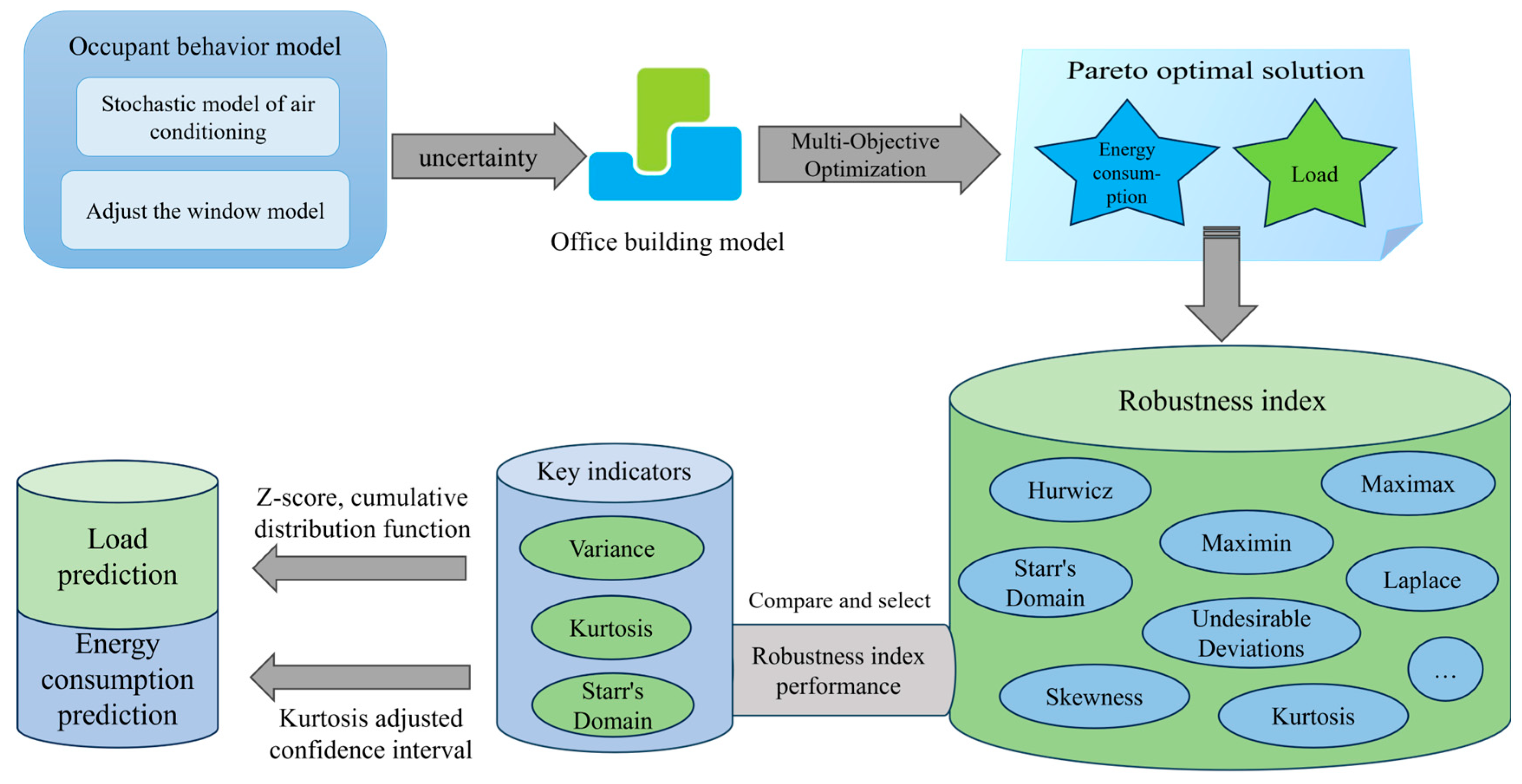
Through this study, we aim to provide practical tools for building designers to better understand and predict the impact of occupant behavior on building energy consumption. Additionally, this research will provide scientific support for developing more effective building energy efficiency policies and promote the development of building energy management strategies, thereby improving energy utilization efficiency. The technology roadmap of this study is shown in Figure 1.

2. Methodology

2.1. Robustness Indicators

Robustness indicators are a set of metrics used to assess the performance of decisions or plans under uncertainty or variability. They aim to measure the resilience of a plan when faced with various possible scenarios. These indicators include trade-offs between optimal and worst-case situations, conservative choices, equal probability evaluations, and the applicability of the plan in multiple situations. Additionally, statistical metrics such as mean, variance, kurtosis, and skewness can be used to evaluate the robustness of a plan. The comprehensive use of these indicators helps decision-makers to better understand the performance of a plan in uncertain environments and make more reliable decisions.

2.1.1. Hurwicz Criterion

The Hurwicz criterion is a decision-making method used in decision theory to handle uncertain situations. Proposed by economist Leonid Hurwicz, this criterion combines both pessimistic and optimistic approaches to decision-making [19]. The calculation process is as follows:

• Determine the Optimism Coefficient (α): This coefficient ranges from 0 to 1, where α represents the decision-maker’s degree of optimism regarding the outcomes. When α = 0, it corresponds to complete pessimism, similar to the Minimax criterion; when α = 1, it represents complete optimism, similar to the Maximax criterion. The optimism coefficient reflects the decision-maker’s attitude towards uncertainty.
• Evaluate the Best and Worst Outcomes for Each Decision: for each feasible decision alternative, identify its best outcome (highest profit or utility) and worst outcome (lowest profit or utility) across all possible states of the environment.
• Apply the Hurwicz Criterion Formula to Compute the Hurwicz Value for Each Decision: for each decision alternative, the Hurwicz value is calculated using the formula:

  Hurwicz = α × Best Outcome + (1 − α) × Worst Outcome

  (1)

  where α is the optimism coefficient, and the best and worst outcomes are the highest and lowest results, respectively, for that decision under all possible scenarios.
• Select the Decision with the Highest Hurwicz Value: compare the Hurwicz values of all decision alternatives and choose the one with the highest value as the final decision.

The key aspect of this method is the selection of the optimism coefficient α, which reflects the decision-maker’s attitude and expectations about future developments. This is a subjective judgment. The actual calculation process is relatively straightforward and simple. By using this approach, the Hurwicz criterion provides decision-makers with a balanced decision-making method that considers both the worst and best possible scenarios. In this paper, we set the optimism coefficient α to 0.5, indicating that the decision-maker has made a balanced judgment between optimism and pessimism.

2.1.2. Maximin Criterion

The Maximin criterion is a decision-making principle used primarily for decision analysis under uncertainty, particularly when considering decisions in the worst-case scenario. This criterion assumes a pessimistic attitude from the decision-maker, who believes that regardless of the chosen decision alternative, the state of nature will always be the most adverse. Therefore, it focuses on minimizing losses or maximizing returns in the worst-case scenario [20]. The calculation process for the Maximin criterion is as follows:

• Determine the Worst Outcome for Each Decision: For each decision option, identify the worst possible outcome among all potential results. This usually involves finding the maximum value within each decision row (if dealing with energy consumption or load) or the maximum loss.
• Select the Maximum of the Worst Outcomes: Among all decision options, choose the one with the largest worst outcome (i.e., the maximum value found in the previous step). This means that, in the worst-case scenario, this decision provides the highest return or the smallest loss.

The Maximin criterion is suitable for extremely conservative decision-makers or in situations where information is so insufficient that predicting various states of nature is difficult. This method ensures that the best possible result is achieved under the most adverse conditions, thereby minimizing risk and loss. In this paper, we will set a threshold for energy consumption and load, with situations below the threshold considered the best case, and the maximum value being the largest value below the threshold.

2.1.3. Maximax Criterion

The Maximax criterion is another decision rule used in decision analysis under uncertainty, assuming that the decision-maker adopts an optimistic attitude. In contrast to the Maximin criterion, it focuses on maximizing the best-case scenario returns, i.e., finding the decision with the highest return in the most favorable situation [21]. The calculation process for the Maximax criterion is as follows:

• Determine the Best Outcome for Each Decision: For each decision option, identify the best possible outcome among all potential results. This usually involves finding the maximum value within each decision row.
• Select the Maximum of the Best Outcomes: Among all decision options, choose the one with the largest, best outcome (i.e., the maximum value found in the previous step). This means that in the best-case scenario, this decision provides the highest return.

The Maximax criterion is suitable for optimistic decision-makers, or when evaluating multiple options, decision-makers tend to consider the highest likely return for each option. This method ensures the highest potential benefit under optimal conditions, thereby maximizing potential gains. However, it may also lead to high risk, as it does not take into account the consequences in poorer scenarios. In this paper, this criterion means the smallest value below the threshold, which is the smallest of all decisions.

2.1.4. Laplace Criterion

The Laplace criterion is a method used in decision theory to handle decision-making under uncertainty. It is based on the assumption that if the decision-maker has no knowledge of the likelihood of various possible future states, then all states are considered equally probable. Therefore, the Laplace criterion recommends selecting the decision with the highest average expected value [22]. The calculation process for this criterion can be broken down into the following steps:

• Calculate the Average Outcome for Each Decision: For each decision option, compute the average of all possible outcomes. This assumes that the probability of each state occurring is equal, so each outcome has the same weight.
• Select the Best Decision: compare the average outcomes of all decision options and choose the one with the highest average value.

The key advantage of the Laplace criterion is its simplicity, as it does not require any prior knowledge of the probabilities of different states. This method is particularly suitable for situations where there is almost complete uncertainty about future states, as it provides a decision-making approach based on a uniform probability distribution. However, this can also be a drawback, as real-world scenarios may involve different probabilities for different outcomes, which the Laplace criterion does not account for. In this paper, we consider the minimum value of the averages for two decisions (energy consumption, load, and thermal comfort).

2.1.5. Starr’s Domain Criterion

Starr’s Domain Criterion, also known as the Domain Criterion, is a method used for decision-making under uncertainty. Proposed by Morris Starr, this criterion aims to address uncertainty in decision-making, especially when the decision-maker has limited knowledge of the probabilities of future events. Starr’s Domain Criterion emphasizes considering the potential outcomes of decisions and their impact on the decision-maker’s objectives, rather than relying solely on probability estimates or expected values.

Unlike the Maximin, Maximax, or Laplace criteria, Starr’s Domain Criterion is less common in decision theory literature and does not have a fixed formula or specific calculation process. Instead, it functions more as a decision framework rather than a precise algorithm with defined steps. Its core idea is to evaluate each decision option across different possible environments and select the most suitable decision based on the decision-maker’s preferences and goals.

The general steps of Starr’s Domain Criterion include:

• Define the Decision Domain: clarify the uncertainty scenarios faced by the decision, including all possible future states or outcomes.
• Evaluate Each Decision Option: for each possible decision option, assess its potential outcomes in various future scenarios.
• Consider the Decision-Maker’s Preferences: analyze the decision-maker’s preferences regarding different outcomes, including value judgments and risk preferences.
• Determine the Optimal Number of Decisions: based on the analysis of possible future environments and the decision-maker’s preferences, identify the decision options that perform best in most scenarios or in the most critical situations.

Therefore, Starr’s Domain Criterion relies more on the subjective judgment of the decision-maker regarding the importance of different decision outcomes and a comprehensive evaluation of each option’s performance across various potential future scenarios. This method is particularly suited for situations where it is difficult to accurately estimate future state probabilities or where the impacts of decisions are complex and variable. In this paper, a threshold will be set, with decisions below this threshold being considered optimal.

2.1.6. Undesirable Deviations Criterion

In the field of building energy conservation, evaluating “undesirable deviations” primarily involves monitoring and analyzing the building’s energy performance to identify instances where energy consumption exceeds expectations or standards. This analysis helps identify potential issues in the design, construction, or operational phases, allowing for measures to be taken to improve the building’s energy efficiency. The calculation of Undesirable Deviations in building energy conservation typically includes the following steps:

• Establish Baseline Energy Consumption

Historical Data Comparison: if the building has been in use for some time, historical energy consumption data can be collected as a baseline. Comparison with Similar Buildings: for new buildings, the baseline can be established by comparing energy consumption with similar buildings in the same region. Standards or Codes: reference national or regional building energy efficiency standards or codes to set the baseline energy consumption.

2.

Energy Consumption Calculation: collect the actual energy consumption data of the building, which typically includes but is not limited to heating, cooling, lighting, and electricity usage.

3.

Calculate the Amount of Undesirable Deviations in Energy Consumption: compare the actual energy consumption with the baseline energy consumption to calculate the amount by which it exceeds the baseline.

2.1.7. Other Statistical Indicators

The Mean Value describes the central point or average level of a set of data. In building energy consumption analysis, calculating the average energy consumption can help us understand the building’s energy or load performance over a certain period, thereby evaluating its energy efficiency and identifying potential energy-saving opportunities.

Variance is a statistical measure that indicates the degree of dispersion in a set of data, representing the average of the squared differences between each data point and the mean of the data set. A larger variance indicates higher volatility in the data; a smaller variance indicates lower volatility. In building energy consumption analysis, calculating the variance can help us understand the fluctuation in energy consumption data, thereby assessing the stability of the building’s energy consumption.

Skewness is a statistical measure that describes the direction and degree of asymmetry in data distribution. Data distribution can be skewed to the left (negative skewness, with the bulk of the distribution concentrated on the right, mean less than the median), skewed to the right (positive skewness, with the bulk of the distribution concentrated on the left, mean greater than the median), or approximately symmetrical (skewness close to 0) [23].

The formula for skewness can be expressed as:

$$g=E{({\displaystyle \frac{\mathrm{x}-\mathsf{\mu }}{\partial }})}^3$$

(2)

where E is the expectation operator, x is each data point in the sample, μ is the sample mean, and $\partial$ is the sample standard deviation.

Kurtosis is a statistical measure that describes the shape characteristics of data distribution, used to assess the peakedness or height of the peak and the thickness of the tails of the distribution. The value of kurtosis reflects the shape characteristics of the data distribution compared to a normal distribution (which has a kurtosis value of 3 in the classical definition). Kurtosis can be positive (kurtosis value greater than 3, indicating a sharper peak and heavier tails than a normal distribution), negative, or zero (relative to the normal distribution) [24].

The formula for sample kurtosis can be expressed as:

$$G=E{({\displaystyle \frac{\mathrm{x}-\mathsf{\mu }}{\partial }})}^4$$

(3)

where E is the expectation operator, x is each data point in the sample, μ is the sample mean, and $\partial$ is the sample standard deviation.

2.2. Comparison of Robustness Indicators

2.2.1. Principles of Comparison

Due to the numerous robustness indicators available and their varying evaluations of data, disagreements can arise. Therefore, it is essential to select the most suitable indicators for evaluating the robustness of data. This study selects two sets of data: annual energy consumption values and annual load values.

To compare the robustness of different indicators, especially when these indicators represent different magnitudes, an effective method is to introduce benchmark values (or ideal values) from statistics as a standard for comparison. These benchmark values represent the ideal or expected performance levels for each indicator. By comparing the actual indicator values with their corresponding benchmark values, we can quantify the relative performance of each indicator. Next, we use the most appropriate value (non-robustness indicator) to calculate the relative dispersion of these data sets and normalize the results reasonably for comparison with robustness indicators. We chose the coefficient of variation to measure the relative dispersion of these data sets. The coefficient of variation provides a method to measure the relative dispersion of data because it is based on the ratio of the standard deviation (a measure of dispersion) to the mean (the average level of the data). The robustness is assessed by comparing the normalized results of the indicators with the coefficient of variation. Specifically, we summarize the following formulas as a measure of robustness, dividing into three cases based on the actual values of the benchmark and indicator values:

If A, B > 0 and A < B:

$$R={\displaystyle \frac{A}{B}}$$

(4)

If B = 0:

$$R={\displaystyle \frac{{10}^x}{{10}^x+A}}$$

(5)

If A, B > 0 and A > B:

$$R={\displaystyle \frac{1}{1+\left|\frac{B-A}{A}\right|}}$$

(6)

where R is the robustness of the indicator, A is the actual value of the indicator, B is the benchmark value of the indicator, and x is the exponent plus 1 of A.

To calculate the proximity of two numbers A and B, where A is the benchmark value, and the maximum proximity is 1, we can define a relative proximity measure that reaches a maximum value of 1 when A and B are exactly equal and decreases as the difference between A and B increases. Considering that A can be greater or smaller than B, we need a symmetric and non-negative measure. A simple and intuitive method is to use the reciprocal of the absolute difference normalized, but this requires handling the case where the denominator may be zero. The above method is an improved approach, considering A can be any value. In this formula, the benchmark value is carefully selected based on the statistical significance and application context of each indicator, reflecting the expected value of the indicator under ideal conditions or target conditions. The actual indicator value is the observed value in the specific context.

A ratio close to 1 indicates that the actual indicator value is very close to the benchmark value, showing that under given conditions, the indicator demonstrates high robustness and can consistently achieve or approach the expected performance level.

A ratio far from 1 indicates that the actual indicator value is significantly different from the benchmark value, suggesting that the indicator may not be stable or has low robustness under current conditions.

By this method, we can not only perform fair comparisons across indicators of different magnitudes but also select the indicator that most closely aligns with the coefficient of variation. This approach helps us identify the most suitable indicator for this study, thereby selecting the most appropriate one.

2.2.2. Benchmark Value

Using the mean as the benchmark value for the Hurwicz criterion, the mean can replace the value of the Laplace criterion, which considers all situations equally likely and selects the best decision by calculating the average. Comparing with the mean can reveal whether the decision rule, after considering the best and worst cases, tends to result in outcomes better or worse than the average situation. If the results obtained by the Hurwicz criterion are close to those obtained by the mean or Laplace criterion, it may indicate that even when considering the impact of the worst case, the energy consumption can still provide robust expected performance.

The benchmark value for variance is the IQR (Interquartile Range). Variance should take the arithmetic square root as the standard deviation because both IQR and standard deviation are indicators of data dispersion, but they have different sensitivities to outliers. IQR focuses on the middle 50% of the data range and is less sensitive to outliers or extreme values, while standard deviation considers the deviations of all data points from the mean, being more sensitive to outliers. If the IQR and standard deviation are similar, it indicates that the data distribution is relatively uniform and that outliers do not significantly affect the overall dispersion of the data. If the standard deviation is significantly larger than the IQR, it may indicate the presence of outliers or extreme values, which increase the overall dispersion of the data.

The benchmark value for Starr’s Domain is 100%. When we set the benchmark for Starr’s Domain Criterion to 100%, it essentially means that we expect the decision options to meet the preset standard or target in all possible scenarios. The closer the score is to the benchmark value, the higher the robustness of the indicator.

The benchmark value for Undesirable Deviations is 0. In statistics, using confidence intervals to assess “Undesirable Deviations” is a feasible method. This approach relies on determining a threshold beyond which observed values are considered outliers or undesirable. By calculating the percentiles of the data (e.g., the 5th percentile and the 95th percentile), the distribution characteristics of the data and the possible range of extreme values can be directly assessed. This method does not rely on estimating the central tendency but directly starts from the distribution characteristics of the data. This means that values beyond this range can be regarded as Undesirable Deviations.

The benchmark value for skewness is 0, and the formula used should be: $R={\displaystyle \frac{1}{1+\left|A\right|}}$. Skewness measures the asymmetry of the data distribution. The ideal skewness value is 0, indicating a perfectly symmetrical distribution. The smaller the skewness, the higher the robustness of the indicator.

The benchmark value for kurtosis is 0, and here we use excess kurtosis: excess kurtosis = |kurtosis − 3|. The purpose of excess kurtosis is to simplify analysis and interpretation, making the kurtosis of a normal distribution 0 instead of 3. This approach makes the normal distribution a neutral benchmark point, facilitating the comparison of kurtosis among different distributions. The value of excess kurtosis indicates the degree of deviation of the data distribution shape from a normal distribution: excess kurtosis greater than 0 (positive excess kurtosis) indicates that the tails of the data distribution are thicker than those of a normal distribution, and the peak of the distribution is sharper. This type of distribution is called “leptokurtic”; excess kurtosis less than 0 (negative excess kurtosis) indicates that the tails of the data distribution are thinner than those of a normal distribution, and the peak of the distribution is flatter. This type of distribution is called “platykurtic”; an excess kurtosis of 0 means that the tail thickness and peak sharpness of the data distribution are similar to those of a normal distribution. Thus, the closer the indicator value is to 0, the higher the robustness.

The benchmark value for Maximin is the minimum value. Maximin represents the best result in the worst-case scenario. Here, we refer to the threshold of Starr’s Domain Criterion mentioned earlier; values greater than this threshold are considered the worst cases, and the minimum value in these worst-case scenarios is the best result.

The benchmark value for Maximax is the minimum value. It represents the best result in the best-case scenario. Here, the best case also refers to the threshold of Starr’s Domain Criterion mentioned earlier; values less than this threshold are considered the best cases, and the minimum value of these is used as the benchmark.

The benchmark value for the mean and Laplace is the minimum value. For these two indicators, the smaller the value, the higher the robustness, but it cannot be 0. Therefore, we refer to the minimum value of the data as the benchmark.

2.3. Energy Consumption and Load Forecasting

2.3.1. Confidence Interval

A confidence interval (CI) is a statistical method used to estimate the possible range of a parameter (such as the mean) and indicate the probability that this range contains the parameter. First, select a confidence level, commonly 90%, 95%, or 99%. The higher the confidence level, the wider the confidence interval, reflecting higher confidence [25]. Next, determine the sample statistics and calculate the sample mean and standard deviation. For large samples (n > 30), use the sample standard deviation; for small samples (n ≤ 30), use the sample standard error (standard deviation divided by $\sqrt{n}$). Then, choose the appropriate distribution. Use the standard normal distribution (Z distribution) for the known population standard deviation and large sample size, and the t distribution for the unknown population standard deviation or small sample size.

The calculation method for confidence intervals is the following: for the Z distribution (applicable to large samples and known population standard deviation), the formula is $\overline{x} \pm$ Z$\partial$, where Z is the critical value of the standard normal distribution corresponding to the selected confidence level (e.g., Z ≈ 1.96 for a 95% confidence level, Z ≈ 1 for a 68% confidence level) [26]; for the t distribution (applicable to small samples or unknown population standard deviation), the formula is $\overline{x} \pm$ ts, where t is the critical value of the t distribution corresponding to the selected confidence level and degrees of freedom (n − 1), and s is the sample standard deviation [27]. Adjust the confidence interval calculation formula according to kurtosis as $\overline{x} \pm$ (Z + Kurtusis)$\partial$.

2.3.2. Z-Score

Unlike simply assuming that the overall load distribution is normal, we also consider Starr’s Domain, which provides a way to investigate the distribution characteristics below a specific threshold, particularly when this threshold is different from the mean, where the value of this approach becomes more pronounced.

Using the concept of Z-scores is a key step in this methodology. The Z-score is a standardized score that describes the relative position of a data point in a standard normal distribution, allowing us to quantitatively compare the threshold with the mean of the overall load distribution. The calculation formula is:

$$Z={\displaystyle \frac{X-\mu }{\partial }}$$

(7)

where X is the value of the data point, μ is the mean of the dataset, and $\partial$ is the standard deviation of the dataset [28]. This study uses the Z-score to estimate the theoretical proportion of the load distribution that does not exceed the threshold, based on the cumulative distribution function (CDF) of the normal distribution.

2.4. Building Model

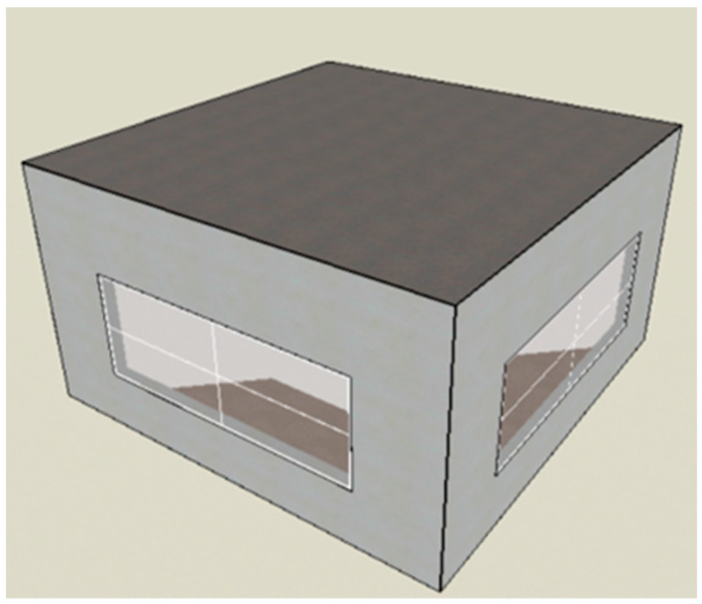
This study focuses on a typical office building, which consists of five rooms. Four of these rooms have windows facing the four cardinal directions: east, west, south, and north. The building is located in Ningbo, a city characterized by hot summers and cold winters. The total floor area is 26.3 square meters. Despite its small size, this model is representative and can be used to study and analyze energy consumption and comfort issues in small office spaces. This small office building model helps in understanding and predicting the energy consumption and comfort characteristics that might occur in larger office buildings through an “extrapolation from small to large” approach. By conducting an in-depth study of this small model, it is possible to quickly and effectively perform energy consumption simulations and evaluations, extracting relevant data and patterns, thereby providing valuable references for energy-saving assessments of large or high-rise office buildings. Figure 2 and Figure 3 below show examples of the model in DesignBuilder (version 7.0.2.004) used in this study.

The building envelope employs typical energy-efficient materials designed to meet the energy efficiency design standards for residential buildings in regions with hot summers and cold winters. The U-values for the exterior walls and roof are set between 0.3–1.2 W/m²K and 0.2–0.8 W/m²K, respectively.

Table 1. Building performance parameters.

Category	Description	Performance Parameters
Exterior Walls	100 mm brick structure + 80 mm XPS + 100 mm concrete block + 10 mm gypsum plaster	U = 0.9 W/m2·K
Exterior Windows	5.7 mm clear glass + 13 mm air gap + 5.7 mm clear glass	U = 3.4 W/m2·K SHGC = 0.6
Roof	10 mm asphalt + 145 mm glass wool + 13 mm gypsum board	U = 0.47 W/m2·K
Ventilation	No mechanical ventilation, natural ventilation at 2.0 h−1
Air Conditioning System	Air conditioning for heating and cooling, design temperatures: heating at 18 °C; cooling at 26 °C	Heating efficiency COP = 1.9 Cooling efficiency EER = 3.4

presents detailed information about the building envelope of this office.

The air conditioning cooling temperature is set to 26 °C, and the heating temperature is set to 18 °C. The energy efficiency ratio (EER) for cooling is 3.4, and the coefficient of performance (COP) for heating is 1.5. The system operates year-round to meet the indoor temperature settings. The ventilation rate is 2.0 air changes per hour. The total power density for other loads (including lighting systems and human activities) is 4.3 W/m². These settings comply with the energy-saving standards for the building.

With these detailed settings, the office building can achieve energy savings while maintaining comfort. The selection of U-values for the building envelope, the EER and COP settings for the air conditioning system, as well as the determination of ventilation rates and power density for other loads, are all based on enhancing overall building energy efficiency and meeting energy-saving standards. This design not only helps reduce energy consumption but also provides a healthy and comfortable working environment for the office. These measures reflect the need to consider various factors comprehensively when designing energy-efficient buildings to achieve the best balance between energy efficiency and comfort.

2.5. Occupant Behavior Model

This study includes a random air conditioning model and a window adjustment model. These models determine the most comfortable settings based on actual occupant behaviors, such as arrival and departure times and the choice to open windows or use air conditioning. This not only provides a realistic simulation of occupant behavior but also achieves energy savings to a certain extent. We use Python scripts to call EnergyPlus (version 23-1-0) API functions and ensure they meet the requirements of the logistic regression model. The core of the logistic regression model is to calculate the p-value based on the average temperature of a specific area, which represents the probability of adjusting the cooling set point. When this probability exceeds a uniformly distributed random value, the cooling set point will be adjusted accordingly. The basic formula of the model is:

$$P(X=x)={\displaystyle \frac{e^{{(\beta }_0+{\beta }_1{x}_1+{\beta }_2{x}_2+\dots {\beta }_n{x}_n)}}{1+e^{{(\beta }_0+{\beta }_1{x}_1+{\beta }_2{x}_2+\dots {\beta }_n{x}_n)}}}$$

(8)

where P (Y = 1|X = x) represents the probability of the event occurring given X. β represents the model parameters that need to be estimated through the maximum likelihood estimation method. X represents the independent variables. The main feature is that it can estimate the probability of an event occurring.

(1)

Stochastic Air Conditioning Model

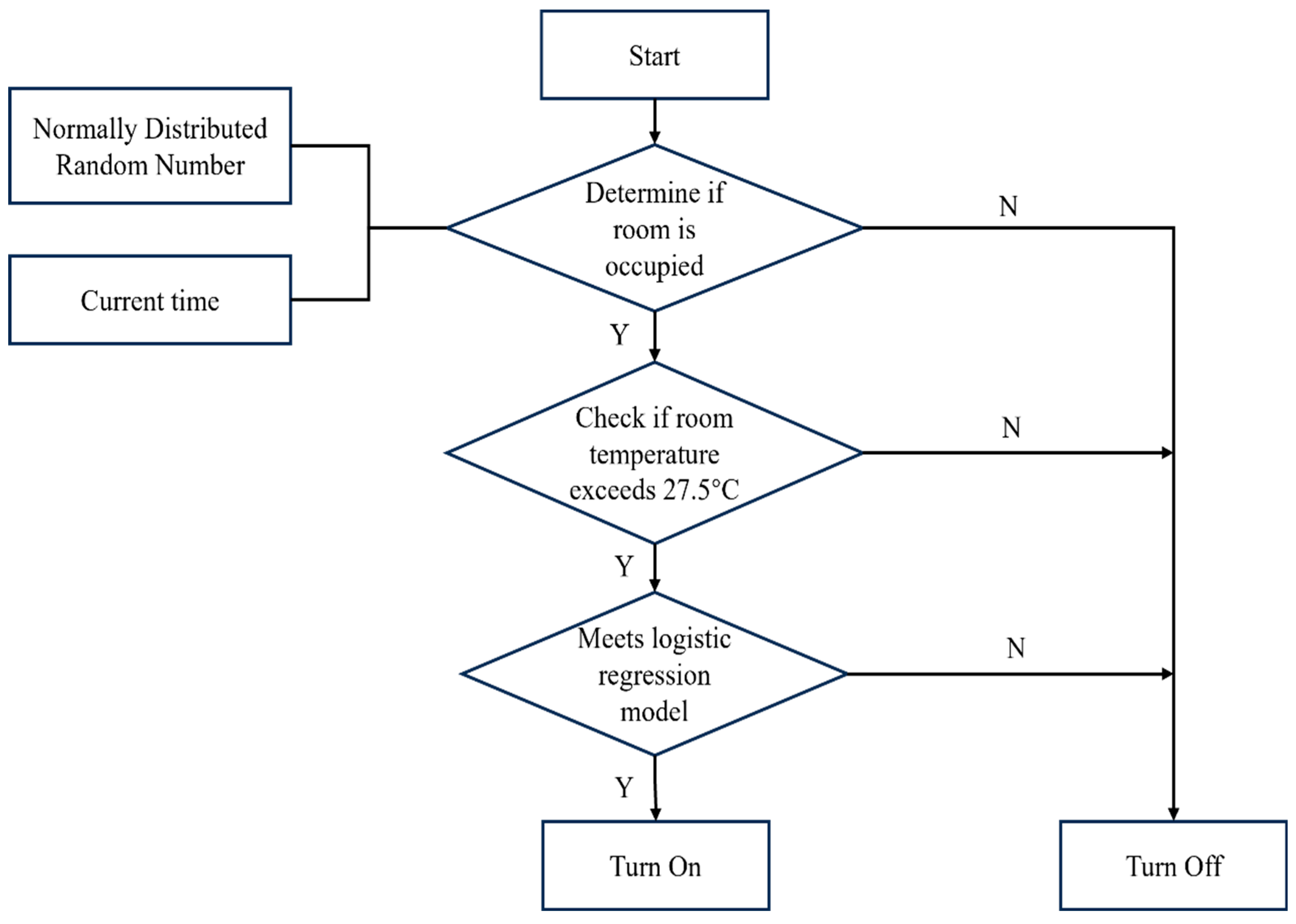
According to research by Wang Chuang [29], the cooling demand of a building is controlled by adjusting the cooling set point. Figure 4 below is a schematic diagram of the air conditioning model.

When the average air temperature in a certain area rises to 27.5 °C, the cooling set point of the air conditioning will be adjusted based on the current time, a normally distributed random number, and the logistic regression model. The air conditioning will turn on if the following conditions are met: first, the current simulation time must be within the range determined by the normally distributed random number; second, the average temperature in the room must exceed 27.5 °C; and, finally, it must meet the requirements of the logistic regression model. It is worth noting that since the seed of the normally distributed random number is determined by the current simulation time in seconds, the simulation time range varies each time, providing a realistic basis for simulating the uncertainty of daily occupant behaviors (such as arrival and departure times).

(2)

Window Adjustment Model

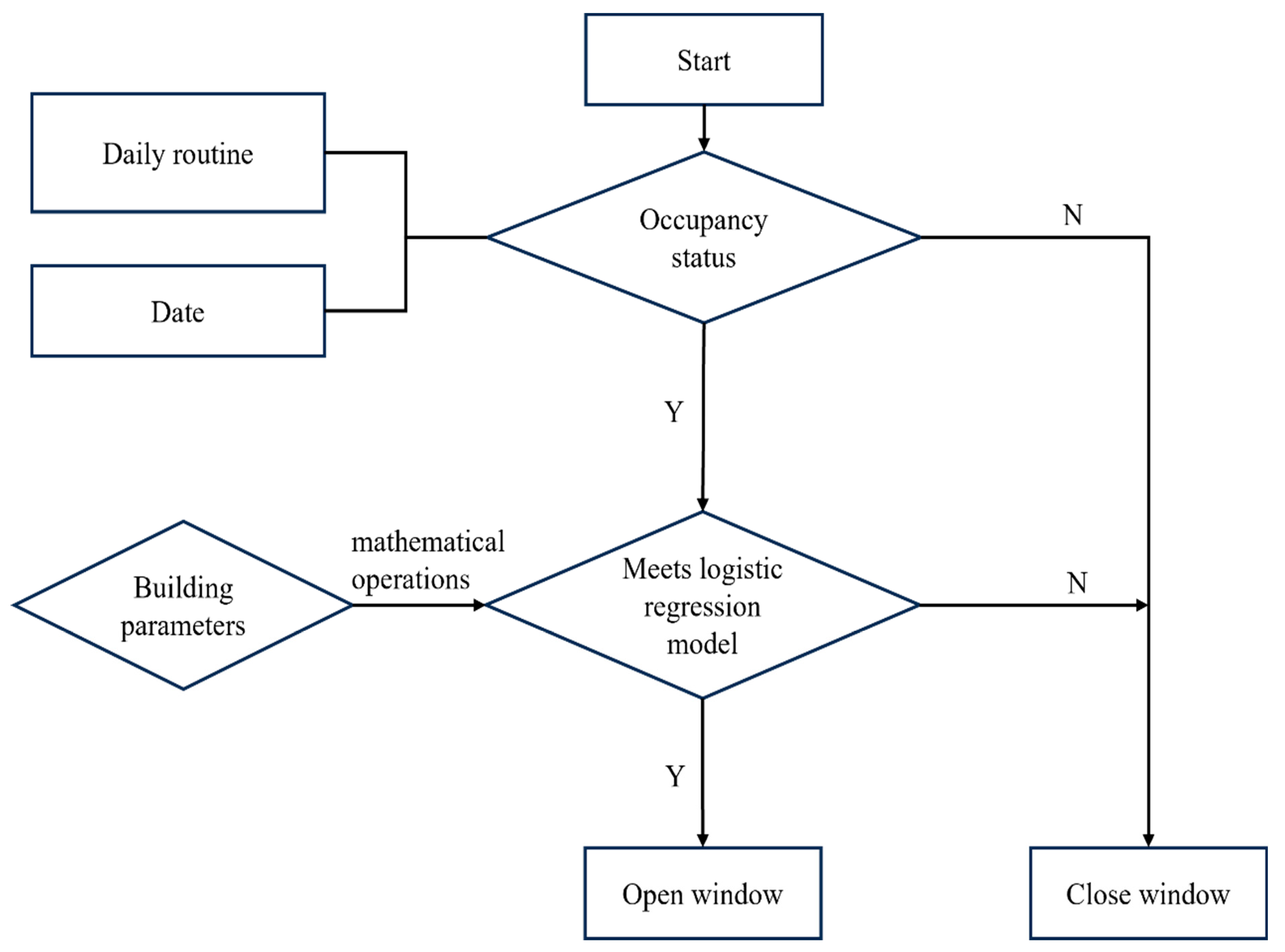
This model takes multiple influencing factors into account. By adjusting the ventilation design flow rate of the zone, we can control the window opening requirements of the building. First, the occupancy of the room is determined based on the days of the week and people’s daily routines. Combining the current time, normally distributed random numbers, and the logistic regression model, the opening and closing state of the windows is adjusted. Figure 5 shows the window adjustment model diagram.

The opening and closing of windows are influenced by multiple conditions:

• Whether the current simulation time meets the normally distributed random number definition.
• Whether it is a Saturday or Sunday.
• Whether the current date is a public holiday.
• Whether it meets the logistic regression model standards.

The generation of random numbers is the same as previously described, used to determine whether there are people in the room. If it is the weekend (Saturday or Sunday), it is assumed that the room is unoccupied. For public holidays, the judgment criteria differ from those of the logistic regression model because the probability of people being in the office is significantly lower during holidays. Additionally, people’s window opening and closing behaviors vary by season. For example, in winter, if the room is too cold, people may choose to close the windows to keep warm; in summer, if it is too hot indoors, people may choose to close the windows and turn on the air conditioning. However, this model considers various factors that might influence the opening and closing of windows, each with different weights. Ultimately, the model uses logistic regression to predict the likelihood of opening the window and decides whether to open the window based on this prediction.

By considering multiple factors influencing window-opening behavior, we can make building energy management more refined and personalized. This behavior-based model approach not only helps save energy but also improves the comfort of the office and work environment.

These occupant behavior models are included as influencing factors in the multi-objective optimization evaluation using NSGA-II.

2.6. Multi-Objective Optimization

2.6.1. Selection of Optimization Objectives

The optimization objectives are chosen to be energy consumption, load, and uncomfortable hours, aiming to find a reasonable balance between energy savings and thermal comfort.

Energy consumption refers to the total energy consumed during building operation for services such as heating, cooling, and lighting; load typically refers to the rate at which equipment, systems, or buildings consume energy or the amount of electricity that power systems need to supply.

Energy consumption can be chosen as an optimization objective because energy consumption is directly related to the operational costs and environmental impact of buildings. Reducing energy consumption not only lowers economic costs but is also crucial for improving building sustainability. Load optimization helps adjust energy supply and demand, optimize energy distribution, and achieve efficient and economical energy use.

Uncomfortable hours are an indicator measuring indoor thermal comfort in buildings, reflecting the total time when indoor temperature conditions deviate from comfort standards. Including uncomfortable hours in the optimization objectives aims to balance improvements in energy efficiency with indoor environmental comfort.

2.6.2. Optimization Variables

Zhang et al. used the Latin Hypercube Sampling (LHS) method, focusing on the impact of nine major building parameter categories on building energy consumption: wall insulation thickness, roof insulation performance, window-to-wall ratio, window glass type, airtightness, solar heat gain coefficients of roofs and walls, occupant density, lighting density, and equipment usage density. Additionally, considering the orientation factor, each room was independently sampled and divided into 33 subcategories. Ultimately, through Sobol sensitivity analysis, 18 variables with higher sensitivity to the results were identified [30]. This study selects these 18 variables for optimization. The variable value ranges, i.e., the constraints, refer to the Zhejiang Province Public Building Energy Efficiency Design Standard DB33/1036-2021 [31]. The specific values are shown in

Table 2. Optimization variables and constraints.

Optimization Variables	Value Range
WindowWallRatio_West	0.1–0.9
WindowWallRatio_North
WindowWallRatio_East
WindowWallRatio_South
PopulationDensity_South	4–16 m2/people
PopulationDensity_North
AirTightness_East	0.1–1
AirTightness_Middle
AirTightness_North
AirTightness_West
AirTightness_South
InsulationThickness_South	0.022–0.158 m
InsulationThickness_North
InsulationThickness_West
GlassSolarAbsorption_South	0.25–0.75
GlassSolarAbsorption_North
GlassSolarAbsorption_East
GlassSolarAbsorption_West

below.

2.6.3. Optimization Method

This study employs the NSGA-II (Non-dominated Sorting Genetic Algorithm II) as the genetic algorithm.

Due to the large computational load and slow execution speed of the original NSGA, Deb et al. introduced NSGA-II in 2002, making improvements in the following three areas:

• NSGA-II uses a fast non-dominated sorting method that reduces the algorithm’s computational complexity from O(mN³) to O(mN²), significantly decreasing computation time.
• In NSGA-II, parent and offspring populations are combined before performing non-dominated sorting. This strategy expands the search space. When selecting parents for the next generation, individuals are chosen based on priority order, and their crowding distance is used to select among individuals at the same level, ensuring a higher retention probability for better individuals.
• The crowding distance method replaces the fitness sharing strategy, which requires specifying a sharing radius. It serves as a criterion for selecting better individuals within the same rank, ensuring diversity within the population. This approach facilitates selection, crossover, and mutation across the entire spectrum of the population.

The NSGA-II parameter configuration used in this study is shown in

Table 3. Parameter configuration for NSGA-II.

Parameters	Value
Population size	35
Maximum number of generations	60
Crossover rate	0.9
Mutation rate	0.1

.

To ensure convergence and a rich set of solutions during the optimization process, the population size was set to 35, which is approximately twice the number of decision variables used in the optimization. The crossover rate and mutation rate were traditionally set to 0.9 and 0.1, respectively. Convergence conditions were based on the researcher’s judgment, and the optimization process was terminated after reaching a maximum of 60 generations.

In addition, to mitigate the impact of uncertainty due to human behavior, this study conducts 100 independent runs for each individual and evaluates the fitness of the individual based on the mean of these samples’ objectives. This method aims to smooth out random fluctuations caused by human factors through repeated experiments, thereby capturing the essence of the optimization problem more accurately and ensuring the stability and accuracy of the obtained solutions.

3. Results

3.1. Occupant Behavior and Pareto-Optimal Solutions

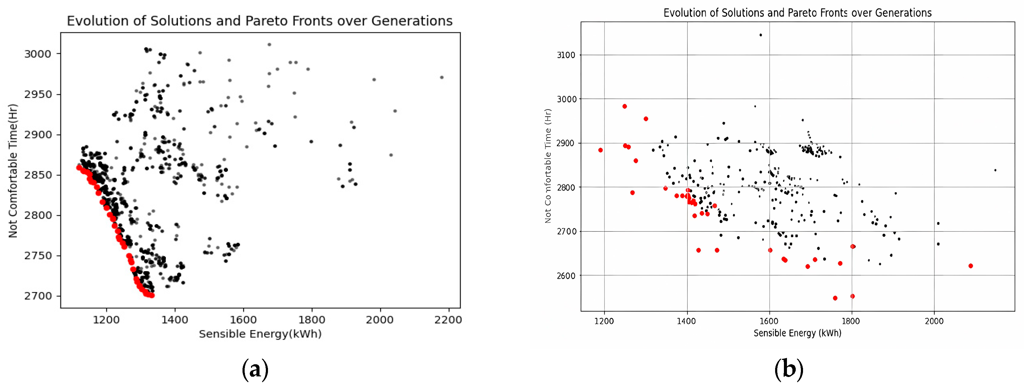
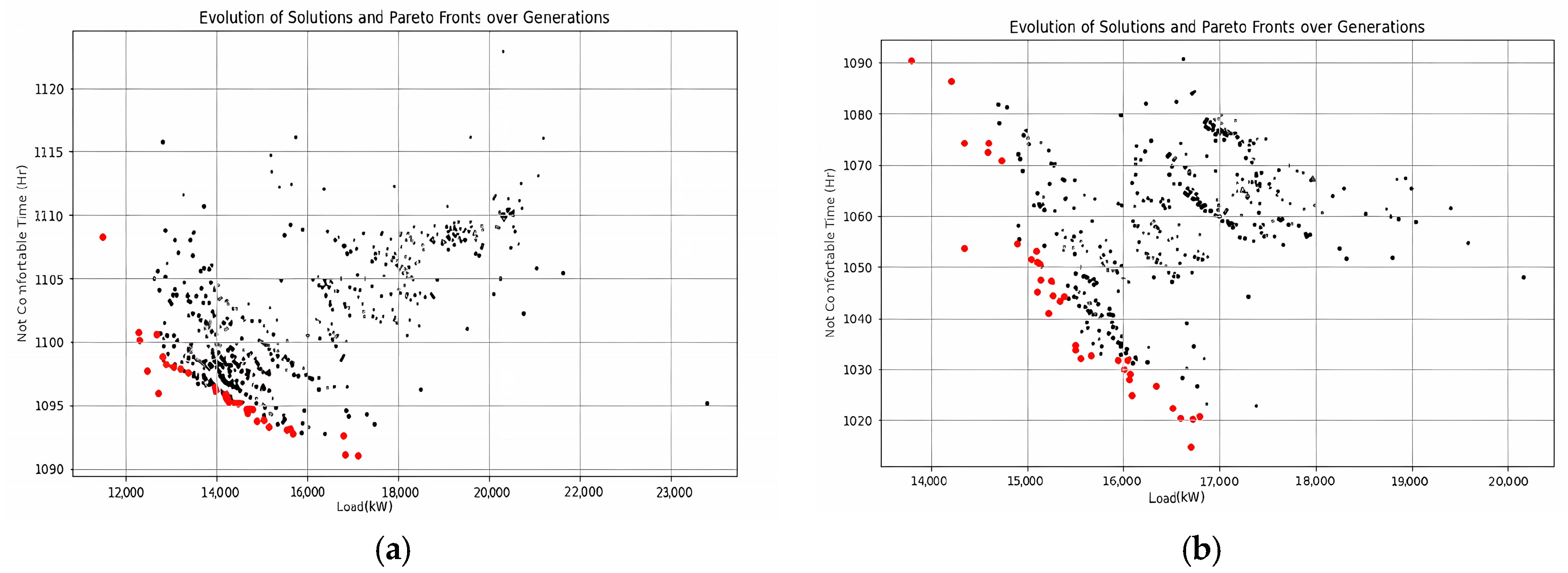
For each individual, the EnergyPlus(version 23-1-0) energy consumption simulation period was from July 1 to September 1, and the climate file for Hangzhou, a region with hot summers, was selected. After 2100 simulations with a population size of 35 and 60 generations of evolution, the assessment strategy produced a distribution of Pareto-optimal solutions. As shown in the figure below, there are a total of 35 Pareto-optimal solutions. Since the behavior of individuals using air conditioning is a crucial random factor, it is essential to evaluate the impact of occupant behavior on building performance. We set up an experimental group and a control group; the former does not consider occupant behavior, with the air conditioning schedule being fixed, while the latter incorporates a stochastic model of occupant behavior.

Figure 6 shows the energy consumption Pareto front without considering occupant behavior versus with consideration of occupant behavior, and Figure 7 shows the load Pareto front under the same conditions. These results are then compared and analyzed.

After the screening process using NSGA-II, the final generation was identified as containing the Pareto-optimal solutions, resulting in a total of 35 optimal solutions. Calculations show that in the model without considering occupant behavior, the average energy consumption of the building was 1245.61 kWh, and the average load was 1232.2 kW. In the model considering occupant behavior, the average energy consumption of the building was 1371.21 kWh, and the average load was 1453.5 kW. From these data, it can be seen that when occupant behavior is considered, the average energy consumption of the building increases by 10.2% and the load increases by 18%.

These data indicate that the uncertainty of occupant behavior increased energy consumption and load. This may be because occupants adjust the air conditioning settings and temperatures according to their own feelings, leading to frequent starts and stops. Each time the air conditioner starts, there is an energy peak, which increases energy consumption. Frequent adjustments may also cause the air conditioner to operate at non-optimal efficiency points, further increasing energy consumption. Occupants may be overly sensitive to indoor and outdoor temperature changes, leading to more frequent and arbitrary use of air conditioning. This not only increases energy consumption but also makes it more unstable. Therefore, we need robust indicators to measure and predict the instability caused by occupant behavior.

3.2. Comparison and Selection of Indicators

3.2.1. Preliminary Calculation

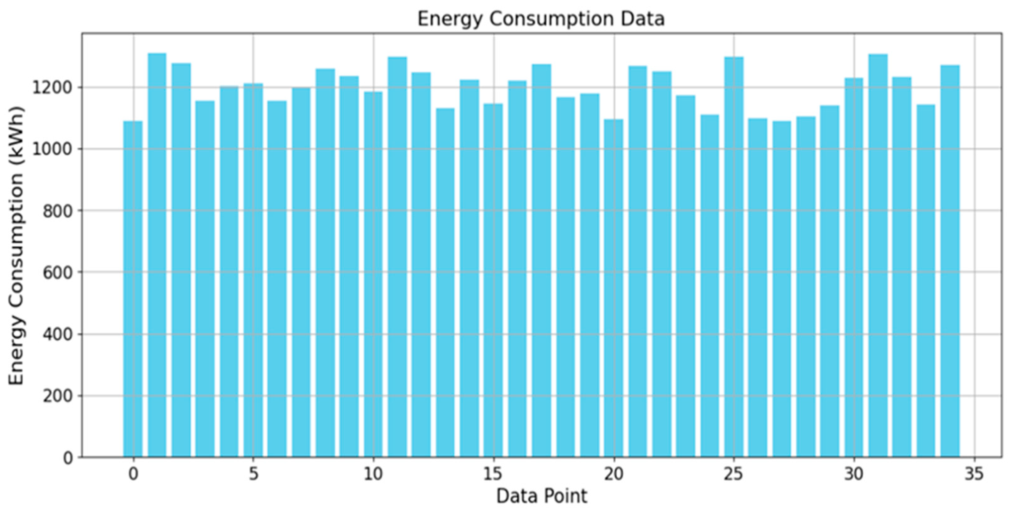
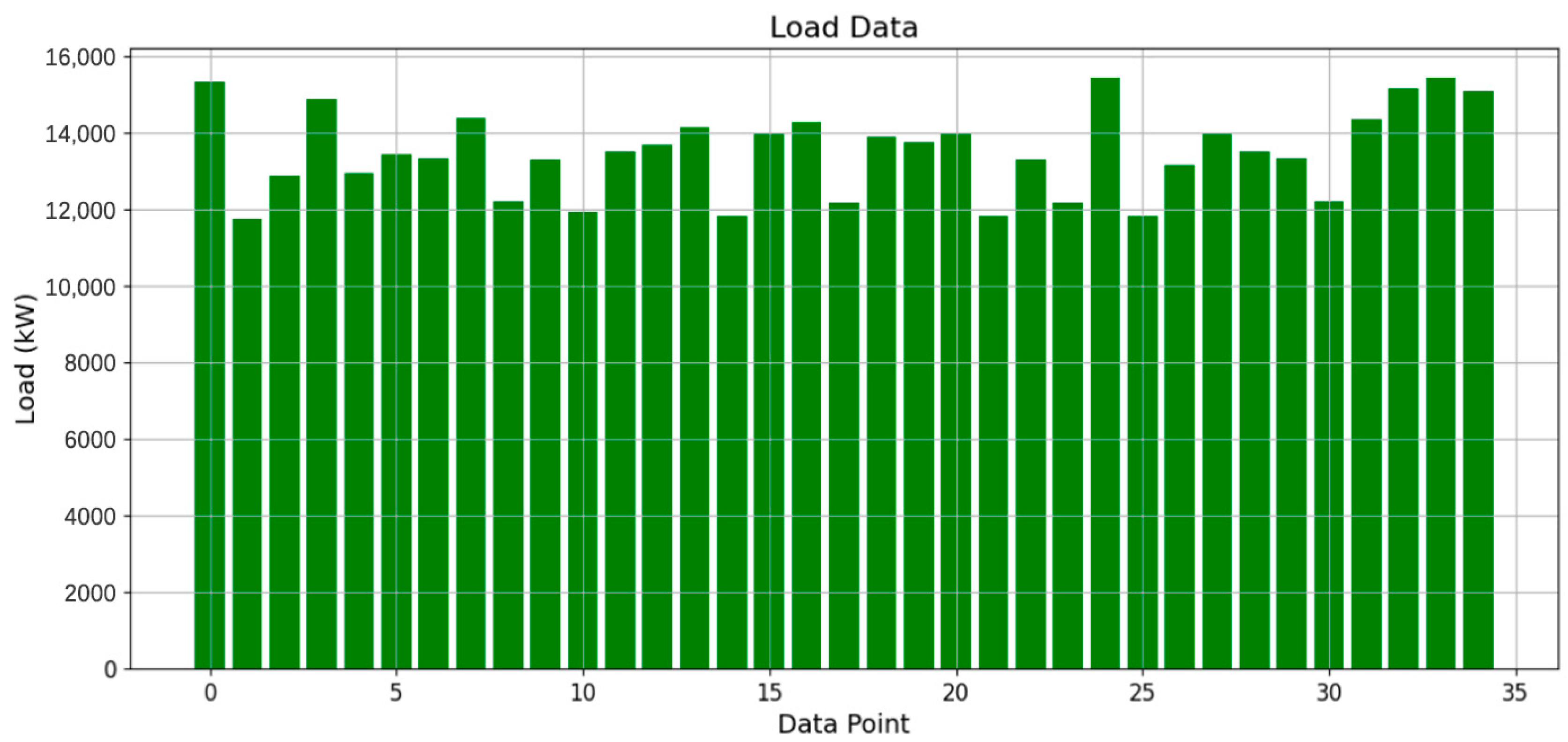
Figure 8 and Figure 9 present the energy consumption values and load values for all Pareto-optimal solutions.

The above consists of 35 energy consumption values and 35 load values, serving as the data source for analysis. For the Hurwicz criterion, the best outcome is represented by the minimum values of both energy consumption and load, while the worst outcome is represented by their respective maximum values. According to the definition of robustness indicators, the calculated values for all indicators are presented in

Table 4. Robustness indicator values.

Robustness Indicators	Energy Consumption	Load
Maximax	1309.39 kWh	11,757.12 kW
Maximin	1087.78 kWh	14,144.61 kW
Hurwicz	1198.58 kWh	13,597.50 kW
Laplace	1198.78 kWh	13,496.59 kW
Mean Value	1198.78 kWh	13,496.59 kW
Variance	4.61 × 105	1.274 × 107
Starr’s Domain	25	25
Undesirable Deviations	2	2
Skewness	−0.08	0.04
Kurtosis	−1.19	−0.95

. These indicator values form the basis for further research, interpretation, and discussion.

From the table above, it can be seen that the Hurwicz, Laplace, and Mean Value indicators are very similar in value because their calculation methods are roughly the same. Starr’s Domain and Undesirable Deviations represent the expected region and Undesirable Deviations, respectively, and they are both measured in units of quantity. The positive and negative signs of skewness represent the distribution of the mean around the peak; for example, the mean of energy consumption data is on the left of the peak, and the mean of load data is on the right of the peak. The positive and negative values of kurtosis represent the concentration or dispersion of the data distribution. The kurtosis of a normal distribution is 3, while the kurtosis of both sets of data is less than three, indicating that the kurtosis is more dispersed than the normal distribution.

3.2.2. Benchmark Values and Calculations

Considering the best and worst cases, for energy consumption, the Hurwicz value is 1198.58 kWh, and the average value is 1198.78 kWh. For load, the Hurwicz value is 13,597.50 kW, and the average value is 13,597.50 kW. The benchmark value for Starr’s Domain is 35. For energy consumption, the threshold is set at the third quartile (Q3) of 1250 kWh, with 25 values below this threshold. For load, the threshold is set at 14,000 kW, with 25 values below this threshold.

To facilitate the assessment of Undesirable Deviations, we count the number of values beyond the deviation. Here, the energy consumption threshold is set at the 95th percentile (1300 kWh), with two values exceeding this threshold. The load threshold is 15,370.83 kW, with two values exceeding this threshold.

For the Maximin, the energy consumption threshold is 1250 kWh, with the minimum value above this threshold being 1251.16 kWh and the overall minimum value being 1087.78 kWh. For load, the threshold is 14,000 kW, with the minimum value above this threshold being 14,144.61 kW and the overall minimum value being 11,757.12 kW.

Regarding variance, the energy consumption variance is 4.61 × 10⁵, the first quartile (Q1) is 1143.44 kWh, and the third quartile (Q3) is 1254.42 kWh, resulting in an interquartile range (IQR) of 109 kWh. The load IQR is 16,737.55 kW, with a standard deviation of 11,287.73 kW. For skewness and kurtosis, the energy consumption data have a skewness of −0.0757 and a kurtosis of −1.186, while the load data have a skewness of 0.0362 and a kurtosis of −0.9458. For mean and Laplace, the energy consumption mean is 1198.78 kWh with a minimum value of 1087.77 kWh, and the load mean is 13,496.59 kW with a minimum value of 11,757.12 kW.

The

Table 5. Performance calculation results of robustness indicators.

Robustness Indicators	Robustness Indicator Performance (Energy Consumption)	Robustness Indicator Performance (Load)
Hurwicz	1	1
Variance	0.59	0.67
Starr’s Domain	0.71	0.71
Undesirable Deviations	0.83	0.83
Skewness	0.56	0.73
Kurtosis	0.70	0.72
Maximin	0.87	0.85
Mean Value	0.91	0.86
Laplace	0.91	0.86

shows the performance calculation results of the robustness indicators.

From the figure above, we can see the performance values of each metric for both load and energy consumption. A value of 1 is the maximum and indicates the best performance of the data under this metric. Lower values indicate poorer performance. However, good performance does not necessarily mean the metric is the most appropriate; the values must also be compared to the actual performance of the data. For example, while the data may perform best under the Hurwicz metric, suggesting no further evaluation is needed, this might not be appropriate. Later, the metrics will be compared to the actual performance of the data to select the most suitable metric values.

3.2.3. Comparison of Indicators

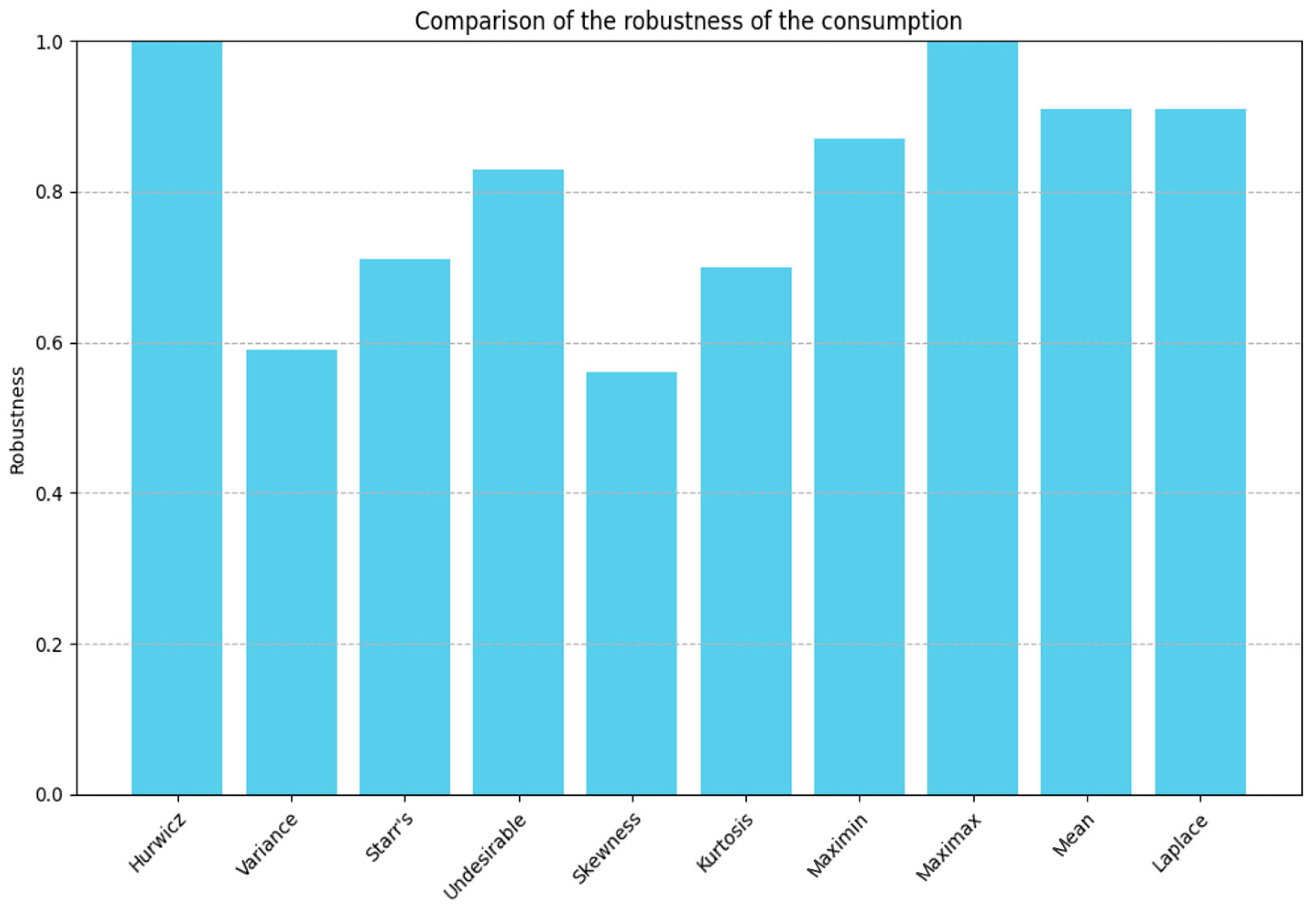
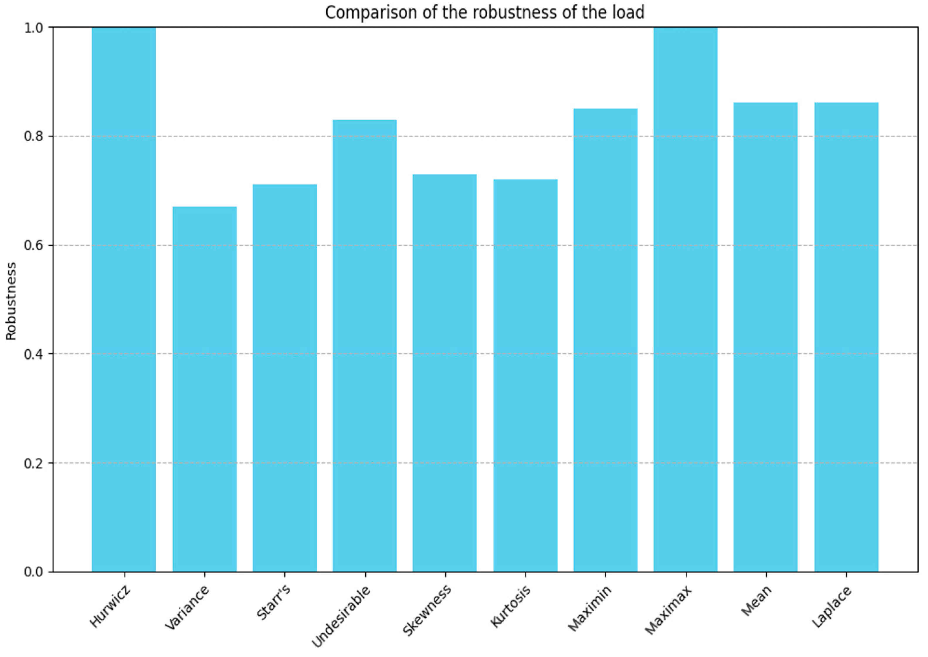
The current data are represented in bar charts, which provide a more intuitive display of the performance of each indicator. This facilitates subsequent observation and comparison. Figure 10 and Figure 11 below show the robustness performance of each indicator for energy consumption and load, respectively.

Next, we need to use the most appropriate value (non-robustness indicator) to calculate the relative dispersion of this data set and reasonably normalize the results for comparison with robustness indicators. We selected the coefficient of variation (CV) to measure the relative dispersion of this data set. The coefficient of variation provides a method for assessing the relative dispersion of data because it is based on the ratio of the standard deviation (a measure of dispersion) to the mean (the average level of data). This makes the coefficient of variation a unitless ratio, which facilitates the comparison of the dispersion of data sets with different units or scales.

The calculated coefficient of variation for energy consumption is CV = 0.05745. When normalized, CV = ${\displaystyle \frac{0.1}{0.1+CV}}$ = 0.635. The coefficient of variation for load is 0.0836, and when normalized, CV = ${\displaystyle \frac{0.1}{0.1+CV}}$ = 0.544. As a measure of relative dispersion, a lower coefficient of variation indicates less fluctuation of the data relative to its mean and thus higher robustness. By comparing the values of the coefficient of variation with other robustness indicators, we can select the robustness indicators that best match the data dispersion. For energy consumption, “Variance” and “Kurtosis” are numerically closest to the coefficient of variation, indicating that these indicators have similar sensitivity to measuring data fluctuation and extreme behavior, and are therefore considered the most suitable for assessing data robustness. For load, we choose “Variance” and “Starr’s Domain”.

Other indicators such as “Maximax” and “Hurwicz” provide valuable information about data characteristics but may not be as closely related to the dispersion and robustness assessment directly associated with the coefficient of variation as “Variance”, “Starr’s Domain”, and “Kurtosis”. They may also not intuitively match the stability and risk sensitivity reflected by the coefficient of variation. However, in Rajesh Kotireddy’s article [32], the “Maximin” indicator was selected, and we will include it in the comparative analysis later.

In summary, “Variance” and “Kurtosis” are chosen as key indicators for assessing the robustness of energy consumption data, while “Variance” and “Starr’s Domain” are selected for assessing the robustness of load data. This choice is based on their close correlation with the coefficient of variation in measuring data dispersion and reflecting data stability. These three indicators collectively provide a comprehensive view of data fluctuation, extreme behavior, and performance under adverse conditions, contributing to the evaluation and enhancement of overall data robustness.

3.3. Energy Consumption Prediction

In the previous section, we selected appropriate robustness indicators. However, to more clearly demonstrate the evaluation results, a numerical comparison of robustness alone is insufficient. We need to further reflect on the target and estimate the target range as accurately as possible to make the results more intuitive. We first perform sample mean approximation optimization for energy consumption and load results and compare the data before and after optimization.

Using statistical principles to estimate the impact of evaluation measures on building energy consumption and load is a scientific and detailed prediction method. By assuming that energy consumption and load results follow a normal distribution, we can use the mean and variance, two core statistical measures, to estimate the range of variation for these indicators. The mean reveals the central point of the data set, while the variance reflects the dispersion of the data.

In building energy consumption and load analysis, considering the uncertainty of actual operations, it is often necessary to introduce a safety margin in the prediction model. For example, by increasing the safety margin from the standard 10% to 15% or 20%, we can more conservatively plan and design the system to handle unexpected load fluctuations or extreme conditions. Assuming data distribution approximates a normal distribution, the mean ± standard deviation (square root of variance) will cover approximately 68% of data points, and the mean ± 2 standard deviations will cover about 95% of data points. Specifically for load analysis, using the mean ± 3 times the standard deviation method can cover most potential extreme values, thereby ensuring system robustness and stability.

However, as the analysis indicates, the actual distribution of energy consumption and load may deviate from a normal distribution due to various factors. In such cases, the use of kurtosis and Starr’s Domain indicators becomes particularly important. The kurtosis indicator helps us understand the sharpness of the data distribution and the thickness of its tails, providing better insight into the sensitivity to outliers. Starr’s Domain, on the other hand, assists in further optimizing the characteristics of the data distribution, especially in the case of deviations from standard distributions.

Therefore, by combining the mean, variance, kurtosis, and potentially Starr’s Domain analysis, we can not only estimate the basic numerical range for energy consumption and load but also gain a deeper understanding of the skewness and extreme values of the distribution. This comprehensive analytical approach provides a solid statistical foundation for ensuring the robustness and adaptability of system design, making optimization measures more precise and effective.

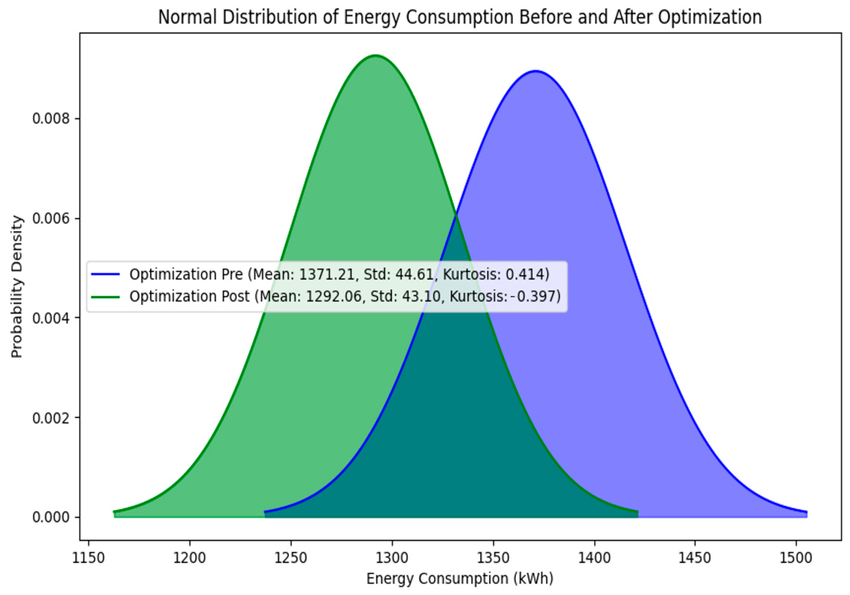
When considering energy consumption analysis, incorporating kurtosis as a key indicator of data distribution characteristics provides a way to gain deeper insight into data volatility. Kurtosis, a statistical measure describing the shape of the data distribution, reveals the frequency of central tendencies and extreme values through their positive or negative values. Specifically, when the kurtosis value is greater than zero, it indicates that the data distribution is more peaked and concentrated compared to a normal distribution, with a higher central peak and thicker tails. This means the data are more concentrated around the mean but also include more extreme values. In such cases, despite most data being tightly clustered around the mean, the presence of extreme values might cause the 95% confidence interval based on the standard deviation to inadequately cover all extreme cases. Conversely, when the kurtosis value is less than zero, it means the data distribution is more dispersed than a normal distribution, with a lower concentration in the central region and a flatter tail. In this distribution pattern, extreme values occur less frequently, and the actual 95% confidence interval appears smaller compared to that of a normal distribution.

To accurately reflect the impact of kurtosis on data distribution, the calculation of the confidence interval is adjusted to mean ± (2 + kurtosis) times the standard deviation. This adjustment accounts for the influence of kurtosis on the shape of the distribution. This method is particularly suitable for data sets with small kurtosis values, close to a normal distribution, and provides a more precise confidence interval estimate compared to traditional methods.

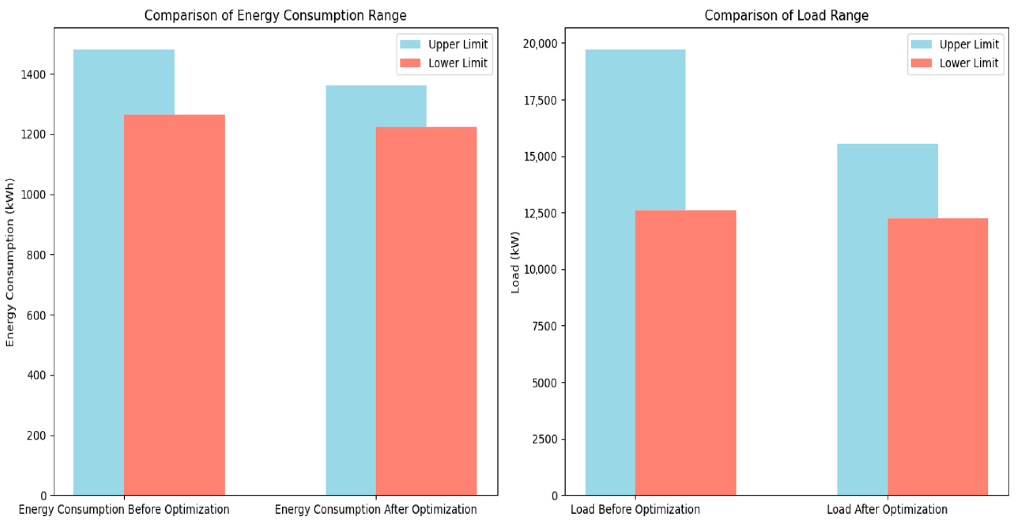
With this optimization, the prediction range for energy consumption has been narrowed from approximately 1263.50 kWh to 1478.92 kWh to between 1222.96 kWh and 1361.16 kWh, demonstrating that the optimized method more effectively controls the uncertainty in energy consumption predictions, offering more reliable data support for energy management and optimization. Figure 12 visually compares the energy consumption distribution before and after optimization, clearly showing the significant improvement in estimation accuracy due to the optimization measures and further validating the importance and effectiveness of considering kurtosis in adjusting the confidence interval for energy consumption analysis.

3.4. Load Prediction

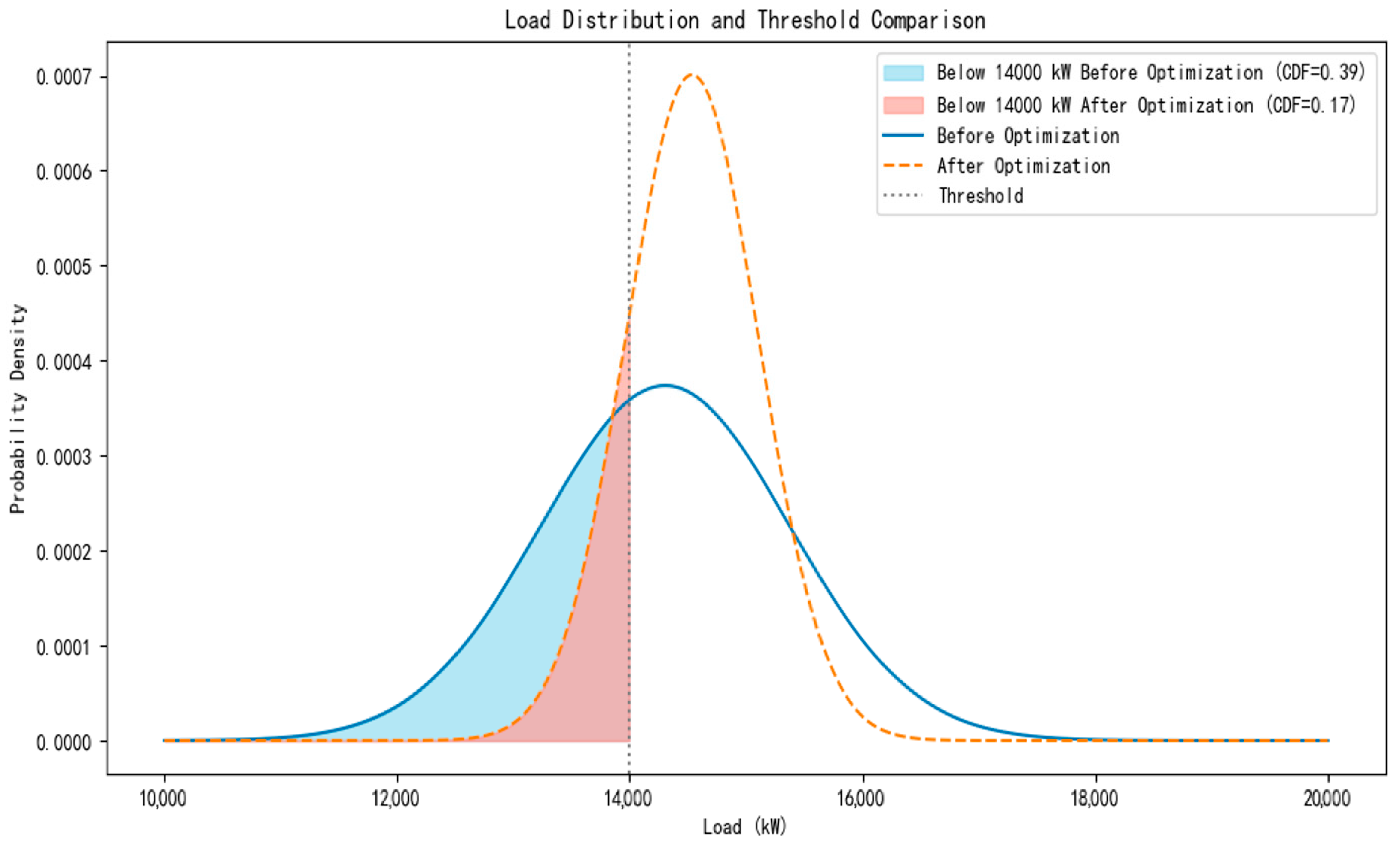
In practice, by counting the number of actual load data points below the threshold and comparing this with the total load count, we can obtain an observed distribution proportion. Comparing this observed proportion with the theoretical distribution proportion calculated using the Z-score reveals the deviation between the actual distribution and theoretical expectations, known as the offset percentage. This offset percentage quantifies the degree to which the actual load distribution deviates from a normal distribution and indicates whether the actual situation exceeds or falls short of the theoretical expectation.

Using this analytical method, we can accurately optimize and refine the load distribution of the power system. The optimized load range is significantly narrowed from the original, approximately 12,578.49 kW to 19,689.42 kW, to a range of 12,217.76 kW to 15,530.56 kW. Figure 13 visually shows the changes in load distribution before and after optimization, providing clear visual evidence of the improvements achieved.

Figure 14 visually compares the prediction ranges of energy consumption and load before and after optimization using the sample mean approximation method, demonstrating the significant improvement in prediction accuracy due to the optimization measures. This comparison clearly shows that both the upper and lower limits of the prediction ranges for energy consumption and load have been markedly reduced, with the reduction in load being particularly notable. This change not only reflects the effectiveness of the optimization method in improving prediction accuracy but also highlights the profound significance of this optimization in enhancing system safety.

In energy management and power system operation, prediction accuracy is directly related to system stability and safety. An overly large prediction range for energy consumption and load can lead to system overload or resource wastage, while a reduced range indicates more accurate predictions of future conditions, allowing for more effective resource allocation and emergency response strategies. Specifically for load prediction, the greater reduction in range means the system can more accurately predict and respond to peak demand periods, thus avoiding the risks of overloading or insufficient power supply, ensuring continuity and reliability in power delivery.

From the figure, we can observe that both energy consumption and load exhibit varying degrees of reduction in both numerical values and ranges before and after optimization. This is especially noticeable in the load predictions, where the optimization results are more pronounced. This confirms the effectiveness of the prediction method.

4. Discussion

When discussing office energy-saving strategies, it is crucial to comprehensively evaluate both energy consumption and load. From a cost-saving perspective, reducing energy consumption directly lowers operating costs, especially through measures such as adopting energy-efficient lighting and high-performance HVAC systems. Additionally, reducing energy consumption helps mitigate the environmental footprint of enterprises, aligning with their environmental responsibility goals and aiding in achieving long-term sustainability objectives such as carbon reduction and energy efficiency improvements.

Load management is another critical aspect of office energy-saving. By optimizing equipment usage schedules and adjusting operating times, excessive energy demand during peak periods can be avoided, leading to optimized energy usage. Effective load management also helps in making more precise decisions regarding infrastructure and equipment investments, such as appropriately sizing air conditioning systems to avoid resource wastage and providing flexibility for potential future office expansions.

Occupant behavior significantly impacts building energy consumption and load, often leading to increases in both. Considering occupant behavior habits in building design and operation can promote more efficient energy use and improve indoor comfort levels.

However, this study has certain limitations. The office building model primarily focuses on energy consumption and load during summer air conditioning, neglecting the related energy consumption during winter heating periods. Future research should include analyses of winter heating systems to comprehensively assess the building’s annual energy efficiency.

The model may not fully capture the complexities of the real world, such as the long-term impacts of climate change, the diversity of building structures (e.g., different materials and designs), and variations in usage patterns. These factors can affect the model’s accuracy and applicability.

In this study, some robustness indicators showed lower performance. However, this does not mean they are irrelevant in practical applications or other fields. Additionally, while the office model used in this study is relatively small, its applicability to high-rise and larger space models requires further investigation. This is particularly important as buildings of different scales and types may face different challenges and demands in terms of energy consumption and indoor environment control. For example, high-rise buildings may exhibit significantly different energy consumption patterns compared to smaller buildings due to unique microclimates, wind pressure differences, and solar radiation factors.

Assumptions about occupant behavior in the model may also have limitations. For instance, the model may assume homogeneous and static occupant behavior, while in reality, behavior can vary due to individual habits, cultural backgrounds, and economic conditions. Additionally, occupant behavior patterns may change over time, which the model might not fully account for.

5. Conclusions

Occupant behavior introduces uncertainty in energy consumption and load, specifically increasing the variability and unpredictability in these areas.

By comparing this with benchmark values, we were able to evaluate and compare different robustness indicators, ultimately identifying the indicators most closely aligned with the coefficient of variation. We determined that the most suitable indicators for evaluating energy consumption are “Variance” and “Starr’s Domain”, while the best indicators for evaluating load are “Kurtosis” and “Variance”.

Utilizing statistical principles, we assumed that the data follow a normal distribution and used the identified robustness indicators to predict energy consumption and load. The results showed that the optimized energy consumption values and ranges were reduced, demonstrating improved robustness.