


A Comparative Study of the Hydrogen Auto-Ignition Process in Oxygen–Nitrogen and Oxygen–Water Vapor Oxidizer: Numerical Investigations in Mixture Fraction Space and 3D Forced Homogeneous Isotropic Turbulent Flow Field


Abstract
1. Introduction
2. Mathematical Modeling
2.1. Unsteady Flamelet Model
2.2. Large Eddy Simulation
3. Numerical Methods
3.1. Solution Method of the Flamelet Equations
3.2. 3D LES/DNS Solver
4. Results
4.1. Auto-Ignition in Mixture Fraction Space
4.2. Auto-Ignition in a 3D Forced HIT
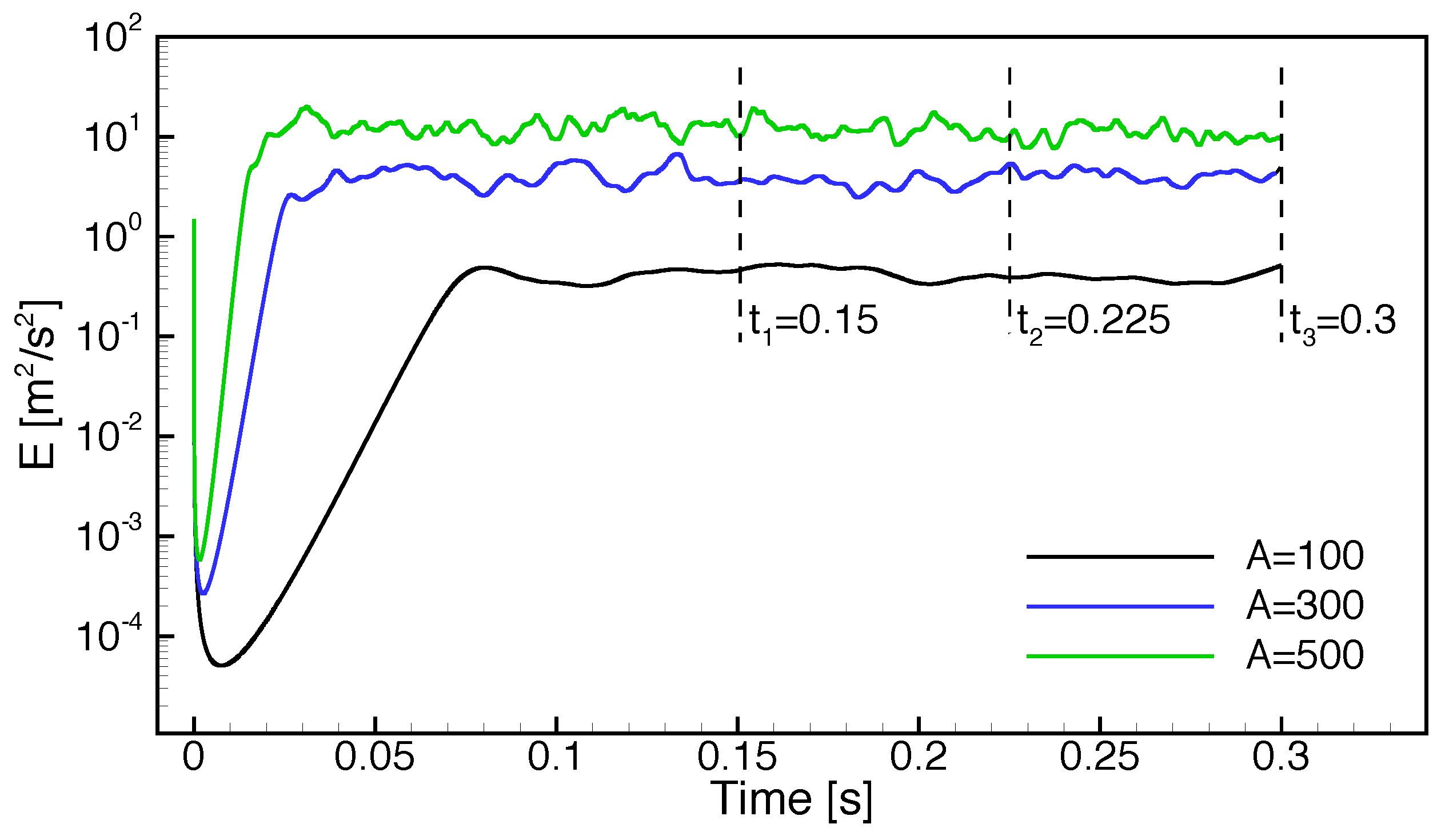
4.2.1. HIT Initialization
4.2.2. Species and Temperature Initialization
4.2.3. Auto-Ignition Process in 3D Forced HIT
5. Conclusions
- is weakly dependent on / when the contents of / in the oxidizer stream are high.
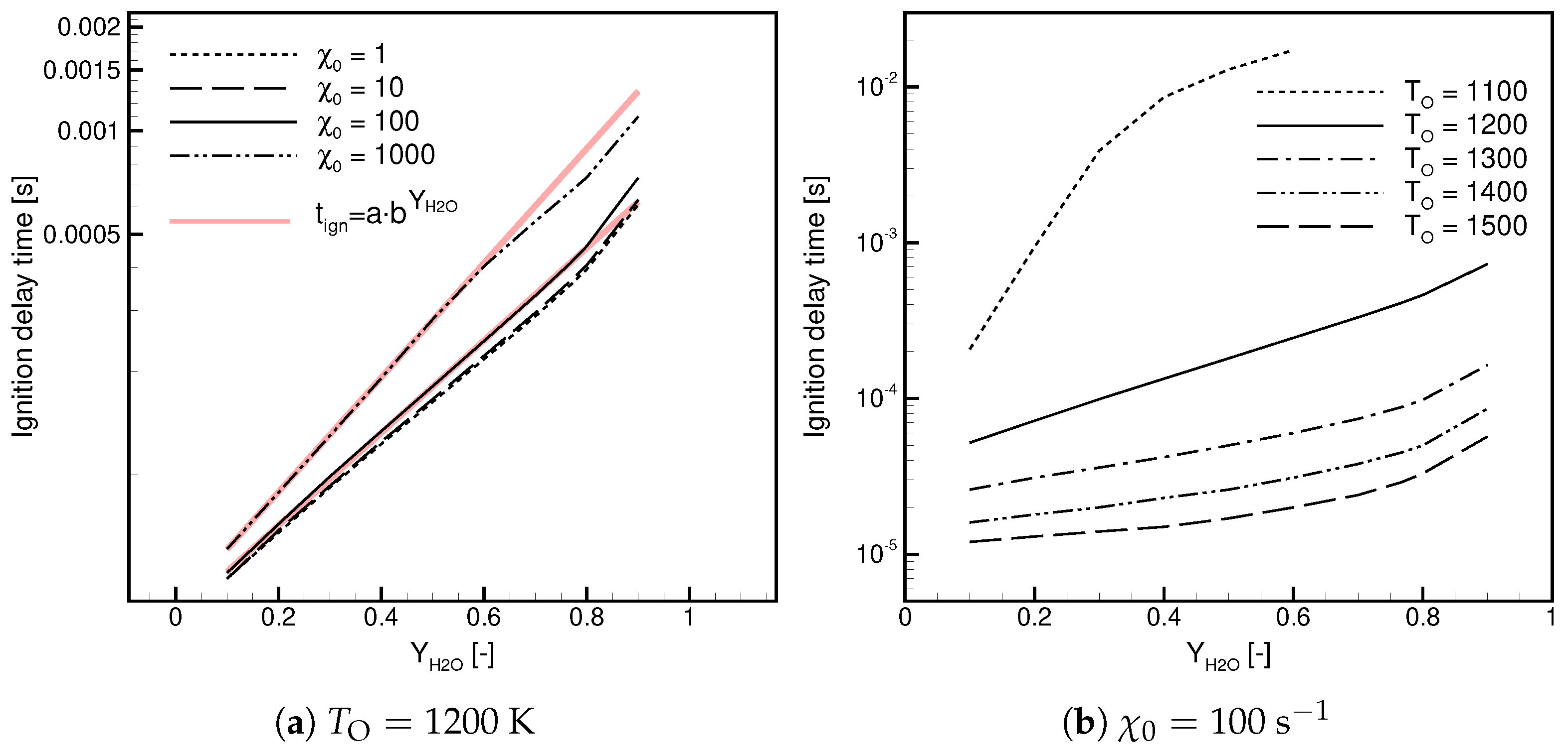
- For Case, decreases with and the temperature.
- For Case, decreases with at a high temperature and shows non-linear behavior in a function of at a low temperature.
- At a low temperature, the ignition delay time for Case is significantly longer; in a lin-log plot, it shows a linear dependence versus .
- At a high temperature, the ignition delay times are similar but the ignitability range in Case is substantially wider.
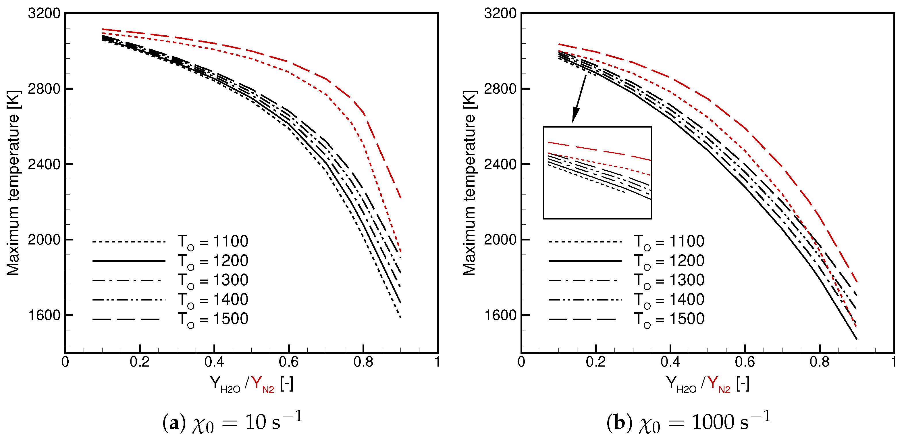
- The maximum temperature decreases with increasing /, and the observed dependence is non-linear.
- The maximum temperature in Case is lower than in Case.
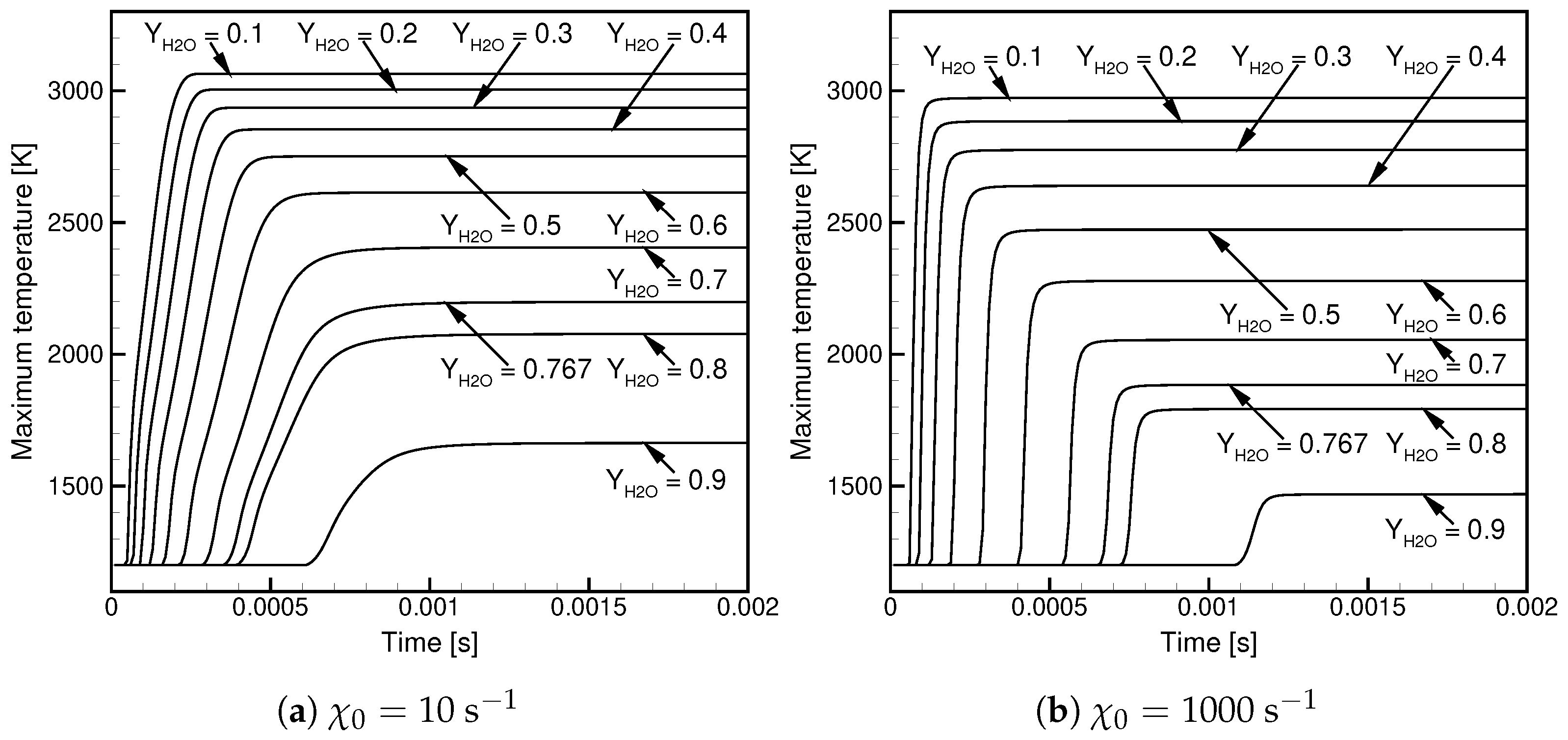
- High values of the scalar dissipation rate delay the ignition and lower the maximum temperature but cause its faster growth in the initial ignition phase.
- Regardless of the oxidizer composition, the ignition occurs in regions of the most reactive mixture fraction where the scalar dissipation rate is low.
- The ignition time is almost independent of the randomness of the initial conditions and turbulence intensity but largely affected by the oxidizer composition and its temperature.
- Case ignite later and the maximum flame temperature in these cases is lower.
- Case exhibit lower ignitability and are more prone to extinction.
Author Contributions
Funding
Institutional Review Board Statement
Informed Consent Statement
Data Availability Statement
Acknowledgments
Conflicts of Interest
Appendix A. Chemical Kinetics

| A [cgs units] | [cal/mol] | |||
|---|---|---|---|---|
| 1. | 1.915 | 0.0 | 16,439 | |
| 2. | 0.508 | 2.67 | 6290 | |
| 3. | 0.216 | 1.51 | 3430 | |
| 4. | 2.970 | 2.02 | 13,400 | |
| 5. | 4.577 | 104,380 | ||
| /2.5//12/ | ||||
| 6. | 6.165 | 0 | ||
| /2.5//12/ | ||||
| 7. | 4.714 | 0 | ||
| 8. | 2.212 | 0 | ||
| /2.5//6.3/ | ||||
| 9. | 1.475 | 0.60 | 0 | |
| LOW/3.482 −1.115/ | ||||
| TROE/0.5 1 1/ | ||||
| /2.5//12/ | ||||
| 10. | 1.66 | 0.0 | 823 | |
| 11. | 7.079 | 0.0 | 295 | |
| 12. | 0.325 | 0.0 | 0 | |
| 13. | 2.890 | 0.0 | ||
| 14. | 4.200 | 0.0 | 11,982 | |
| DUPLICATE | ||||
| 1.300 | 0.0 | |||
| 15. | 2.951 | 0.0 | 48,430 | |
| LOW/1.202 0.0 4.55/ | ||||
| TROE/0.5 1 1/ | ||||
| /2.5//12/ | ||||
| 16. | 0.241 | 0.0 | 3970 | |
| 17. | 0.482 | 0.0 | 7950 | |
| 18. | 9.550 | 2.0 | 3970 | |
| 19. | 1.000 | 0.0 | 0 | |
| DUPLICATE | ||||
| 5.800 | 0.0 | 9557 |
| A [cgs units] | [cal/mol] | |||
|---|---|---|---|---|
| 1. | 3.547 | 16,599 | ||
| 2. | 0.508 | 2.67 | 6290 | |
| 3. | 0.216 | 1.51 | 3430 | |
| 4. | 2.970 | 2.02 | 13,400 | |
| 5. | 4.577 | 104,380 | ||
| /2.5//12/ | ||||
| /1.9//3.8/ | ||||
| /0.0//0.0/ | ||||
| 6. | 6.165 | 0 | ||
| /2.5//12/ | ||||
| /0.0//0.0/ | ||||
| /1.9//3.8/ | ||||
| 7. | 4.714 | 0 | ||
| /2.5//12/ | ||||
| /0.75//0.75/ | ||||
| /1.9//3.8/ | ||||
| 8. | 3.800 | 0 | ||
| /2.5//12/ | ||||
| /0.38//0.38/ | ||||
| /1.9//3.8/ | ||||
| 9. | 1.475 | 0.60 | 0 | |
| LOW/6.366 5.248/ | ||||
| TROE/0.8 1 1/ | ||||
| /2.0//11/ | ||||
| /0.78//1.9//3.8/ | ||||
| 10. | 1.66 | 0.0 | 823 | |
| 11. | 7.079 | 0.0 | 295 | |
| 12. | 0.325 | 0.0 | 0 | |
| 13. | 2.890 | 0.0 | ||
| 14. | 4.200 | 0.0 | 11,982 | |
| DUPLICATE | ||||
| 1.300 | 0.0 | |||
| 15. | 2.951 | 0.0 | 48,430 | |
| LOW/1.202 0.0 4.55/ | ||||
| TROE/0.5 1 1/ | ||||
| /2.5//12/ | ||||
| /1.9//3.8/ | ||||
| /0.64//0.64/ | ||||
| 16. | 0.241 | 0.0 | 3970 | |
| 17. | 0.482 | 0.0 | 7950 | |
| 18. | 9.550 | 2.0 | 3970 | |
| 19. | 1.000 | 0.0 | 0 | |
| DUPLICATE | ||||
| 5.800 | 0.0 | 9557 |
Appendix B
| 0.1 | 0.2 | 0.3 | 0.4 | 0.5 | 0.6 | 0.7 | 0.767 | 0.8 | 0.9 | ||
|---|---|---|---|---|---|---|---|---|---|---|---|
| TO | |||||||||||
| 900 | - | - | - | - | - | - | - | - | - | - | |
| 1000 | 3.3/3.4 | 3.3/3.4 | 3.3/3.4 | 3.3/3.3 | 3.3/3.3 | 3.2/3.3 | 3.2/3.2 | 3.1/3.1 | 3.0/3.0 | 2.7/2.7 | |
| 1100 | 5.4/5.3 | 5.6/5.1 | 5.4/5.0 | 5.3/5.0 | 5.3/4.9 | 5.0/4.8 | 5.0/4.6 | 4.6/4.4 | 4.6/4.2 | 4.0/3.7 | |
| 1100(D) | 5.6/5.4 | 5.6/5.2 | 5.4/5.0 | 5.4/5.2 | 5.2/5.0 | 5.2/5.0 | 5.0/4.8 | 4.8/4.4 | 4.6/4.4 | 4.0/3.8 | |
| 1200 | 6.8/6.2 | 7.2/6.5 | 6.7/6.0 | 6.7/5.9 | 6.5/5.8 | 6.4/5.6 | 5.9/5.5 | 5.7/5.2 | 5.6/5.1 | 4.8/4.2 | |
| 1300 | 8.0/7.3 | 7.7/6.7 | 7.8/6.6 | 7.4/7.0 | 7.8/6.5 | 7.1/6.5 | 6.9/6.1 | 6.7/5.7 | 6.2/5.4 | 5.4/4.7 | |
| 1300(D) | 8.0/7.2 | 8.6/6.8 | 7.8/6.6 | 8.2/7.0 | 7.8/6.6 | 7.2/6.4 | 7.0/6.0 | 6.6/5.8 | 6.6/5.8 | 5.6/4.6 | |
| 1400 | 8.7/7.6 | 8.8/7.7 | 8.9/7.3 | 8.6/7.2 | 8.4/6.9 | 8.1/6.6 | 7.7/6.6 | 7.1/6.3 | 7.2/5.9 | 6.0/4.8 | |
| 1500 | 9.9/8.1 | 9.6/7.7 | 9.6/7.4 | 9.5/7.7 | 9.1/7.3 | 8.6/7.0 | 8.1/6.4 | 8.0/6.3 | 8.0/6.6 | 6.6/5.1 | |
| 0.1 | 0.2 | 0.3 | 0.4 | 0.5 | 0.6 | 0.7 | 0.767 | 0.8 | 0.9 | ||
|---|---|---|---|---|---|---|---|---|---|---|---|
| TO | |||||||||||
| 900 | - | - | - | - | - | - | - | - | - | - | |
| 1000 | 0.330/0.339 | 0.345/0.343 | 0.358/0.356 | 0.374/0.371 | 0.396/0.392 | 0.427/0.422 | 0.475/0.471 | 0.527/0.523 | 0.564/0.561 | 0.808/0.812 | |
| 1100 | 0.079/0.070 | 0.084/0.074 | 0.089/0.079 | 0.096/0.086 | 0.105/0.094 | 0.117/0.106 | 0.136/0.124 | 0.158/0.144 | 0.172/0.157 | 0.266/0.248 | |
| 1200 | 0.037/0.031 | 0.039/0.033 | 0.043/0.035 | 0.048/0.047 | 0.052/0.043 | 0.058/0.048 | 0.069/0.058 | 0.078/0.069 | 0.088/0.074 | 0.138/0.190 | |
| 1300 | 0.023/0.017 | 0.025/0.018 | 0.026/0.020 | 0.029/0.022 | 0.032/0.024 | 0.036/0.027 | 0.042/0.032 | 0.049/0.038 | 0.054/0.042 | 0.085/0.068 | |
| 1400 | 0.015/0.010 | 0.017/0.012 | 0.018/0.012 | 0.020/0.014 | 0.022/0.015 | 0.025/0.017 | 0.029/0.020 | 0.034/0.024 | 0.037/0.026 | 0.059/0.042 | |
| 1500 | 0.011/0.007 | 0.012/0.006 | 0.013/0.008 | 0.015/0.009 | 0.016/0.010 | 0.018/0.012 | 0.022/0.014 | 0.025/0.016 | 0.028/0.018 | 0.045/0.028 | |
| 0.1 | 0.2 | 0.3 | 0.4 | 0.5 | 0.6 | 0.7 | 0.767 | 0.8 | 0.9 | ||
|---|---|---|---|---|---|---|---|---|---|---|---|
| TO | |||||||||||
| 900 | - | - | - | - | - | - | - | - | - | - | |
| 1000 | - | - | - | - | - | - | - | - | - | - | |
| 1100 | 4.2/4.2 | 2.9/3.3 | 1.8/2.3 | 1.7/2.7 | 2.2/3.3 | 2.6/3.8 | 3.0/4.3 | 3.2/4.6 | 3.4/4.8 | 3.9/5.2 | |
| 1100(D) | 4.2/4.2 | 3.0/3.2 | 1.8/2.4 | 1.8/2.8 | 2.2/3.4 | 2.6/3.8 | 3.0/4.4 | 3.2/4.6 | 3.4/4.8 | 3.8/5.2 | |
| 1200 | 6.4/6.2 | 6.2/5.7 | 7.8/5.5 | 5.3/5.1 | 4.9/4.8 | 4.2/4.3 | 4.5/4.5 | 4.0/4.1 | 3.9/4.0 | 3.6/3.7 | |
| 1300 | 7.7/7.0 | 7.9/6.9 | 7.9/7.1 | 7.7/7.1 | 7.7/7.0 | 7.4/6.8 | 6.5/7.0 | 7.3/6.5 | 7.1/6.4 | 6.5/5.8 | |
| 1300(D) | 7.8/6.9 | 7.9/6.9 | 7.9/7.2 | 7.8/7.2 | 7.8/6.9 | 7.9/6.9 | 7.8/6.8 | 7.6/6.8 | 7.4/6.6 | 6.8/5.9 | |
| 1400 | 8.6/7.7 | 9.1/7.7 | 9.7/7.9 | 9.1/8.1 | 9.3/8.6 | 9.3/8.0 | 8.0/7.0 | 9.4/7.6 | 9.4/7.6 | 8.7/6.9 | |
| 1500 | 10/8.1 | 9.9/7.9 | 10/8.9 | 11/8.6 | 11/8.7 | 11/8.4 | 10/6.5 | 11/8.2 | 11/8.3 | 10/7.8 | |
| 0.1 | 0.2 | 0.3 | 0.4 | 0.5 | 0.6 | 0.7 | 0.767 | 0.8 | 0.9 | ||
|---|---|---|---|---|---|---|---|---|---|---|---|
| TO | |||||||||||
| 1100 | 4.6/4.5 | 3.3/3.6 | 2.2/2.7 | 1.6/2.5 | 1.9/3.0 | 2.3/3.5 | 2.6/4.0 | 2.8/4.3 | 3.0/4.4 | 3.4/4.9 | |
| 1100(D) | 4.6/4.6 | 3.4/3.6 | 2.2/2.6 | 1.6/2.4 | 2.0/3.0 | 2.2/3.6 | 2.6/4.0 | 2.8/4.2 | 3.0/4.4 | 3.4/4.8 | |
| 1300 | 7.9/7.6 | 7.9/7.2 | 8.1/7.0 | 8.1/7.1 | 8.4/7.5 | 8.1/7.2 | 8.0/7.2 | 7.7/6.7 | 7.5/6.8 | 7.1/5.9 | |
| 1300(D) | 8.6/7.6 | 8.6/7.2 | 8.2/7.6 | 8.2/7.2 | 8.2/7.4 | 7.9/7.2 | 7.8/6.9 | 7.6/6.9 | 7.8/6.6 | 6.9/6.2 | |
| 0.1 | 0.2 | 0.3 | 0.4 | 0.5 | 0.6 | 0.7 | 0.767 | 0.8 | 0.9 | ||
|---|---|---|---|---|---|---|---|---|---|---|---|
| TO | |||||||||||
| 900 | - | - | - | - | - | - | - | - | - | - | |
| 1000 | - | - | - | - | - | - | - | - | - | - | |
| 1100 | 0.179/0.174 | 0.611/0.656 | 2.179/2.592 | 4.974/5.731 | 7.261/8.034 | 9.041/9.836 | 10.59/11.42 | 11.63/12.42 | 12.16/12.93 | 14.12/14.68 | |
| 1200 | 0.049/0.043 | 0.068/0.059 | 0.092/0.083 | 0.123/0.130 | 0.163/0.152 | 0.216/0.205 | 0.288/0.276 | 0.353/0.341 | 0.394/0.380 | 0.606/0.585 | |
| 1300 | 0.026/0.020 | 0.030/0.024 | 0.035/0.028 | 0.041/0.034 | 0.048/0.040 | 0.057/0.048 | 0.071/0.059 | 0.084/0.071 | 0.094/0.079 | 0.153/0.131 | |
| 1400 | 0.016/0.012 | 0.018/0.013 | 0.020/0.015 | 0.023/0.017 | 0.026/0.019 | 0.030/0.023 | 0.037/0.028 | 0.044/0.034 | 0.049/0.038 | 0.082/0.063 | |
| 1500 | 0.012/0.008 | 0.012/0.008 | 0.014/0.009 | 0.015/0.010 | 0.017/0.012 | 0.020/0.014 | 0.024/0.017 | 0.029/0.020 | 0.032/0.022 | 0.055/0.038 | |
Appendix C
| 0.1 | 0.2 | 0.3 | 0.4 | 0.5 | 0.6 | 0.7 | 0.767 | 0.8 | 0.9 | ||
|---|---|---|---|---|---|---|---|---|---|---|---|
| TO | |||||||||||
| 900 | - | - | - | - | - | - | - | - | - | - | |
| 1000 | - | - | - | - | - | - | - | - | - | - | |
| 1100 | 0.181/0.174 | 0.621/0.664 | 2.244/2.568 | 5.060/5.615 | 7.462/8.091 | 9.361/10.04 | 11.03/11.72 | 12.12/12.81 | 12.70/13.35 | 14.76/15.23 | |
| 1200 | 0.049/0.043 | 0.068/0.059 | 0.092/0.083 | 0.123/0.130 | 0.163/0.153 | 0.217/0.206 | 0.289/0.277 | 0.355/0.0342 | 0.396/0.382 | 0.609/0.588 | |
| 1300 | 0.026/0.020 | 0.030/0.024 | 0.035/0.028 | 0.041/0.034 | 0.048/0.039 | 0.057/0.048 | 0.071/0.059 | 0.084/0.071 | 0.094/0.080 | 0.153/0.134 | |
| 1400 | 0.016/0.012 | 0.018/0.013 | 0.020/0.015 | 0.023/0.017 | 0.026/0.019 | 0.030/0.023 | 0.037/0.028 | 0.044/0.034 | 0.049/0.038 | 0.082/0.063 | |
| 1500 | 0.012/0.008 | 0.012/0.008 | 0.014/0.009 | 0.015/0.010 | 0.017/0.012 | 0.020/0.014 | 0.024/0.017 | 0.029/0.020 | 0.032/0.022 | 0.055/0.038 | |
| 0.1 | 0.2 | 0.3 | 0.4 | 0.5 | 0.6 | 0.7 | 0.767 | 0.8 | 0.9 | ||
|---|---|---|---|---|---|---|---|---|---|---|---|
| TO | |||||||||||
| 900 | - | - | - | - | - | - | - | - | - | - | |
| 1000 | - | - | - | - | - | - | - | - | - | - | |
| 1100 | 0.185/0.178 | 0.672/0.705 | 2.450/2.615 | 5.442/5.733 | 8.237/8.617 | 10.53/10.96 | 12.55/12.99 | 13.87/14.30 | 14.55/14.95 | 16.93/17.18 | |
| 1200 | 0.049/0.043 | 0.069/0.059 | 0.093/0.083 | 0.125/0.139 | 0.166/0.155 | 0.222/0.210 | 0.296/0.284 | 0.365/0.0351 | 0.407/0.392 | 0.629/0.608 | |
| 1300 | 0.026/0.020 | 0.030/0.024 | 0.035/0.029 | 0.041/0.034 | 0.048/0.039 | 0.057/0.048 | 0.071/0.059 | 0.085/0.072 | 0.094/0.080 | 0.155/0.132 | |
| 1400 | 0.016/0.012 | 0.018/0.013 | 0.020/0.015 | 0.023/0.017 | 0.026/0.019 | 0.030/0.023 | 0.037/0.028 | 0.044/0.034 | 0.049/0.038 | 0.082/0.063 | |
| 1500 | 0.012/0.008 | 0.012/0.008 | 0.014/0.009 | 0.015/0.010 | 0.017/0.012 | 0.020/0.014 | 0.024/0.017 | 0.029/0.020 | 0.032/0.022 | 0.055/0.038 | |
| 0.1 | 0.2 | 0.3 | 0.4 | 0.5 | 0.6 | 0.7 | 0.767 | 0.8 | 0.9 | ||
|---|---|---|---|---|---|---|---|---|---|---|---|
| TO | |||||||||||
| 900 | - | - | - | - | - | - | - | - | - | - | |
| 1000 | - | - | - | - | - | - | - | - | - | - | |
| 1100 | 0.207/0.199 | 0.939/0.954 | 3.899/4.001 | 8.591/9.297 | 12.93/16.35 | 17.23/18.97 | - | - | - | - | |
| 1200 | 0.052/0.044 | 0.072/0.063 | 0.099/0.088 | 0.134/0.123 | 0.181/0.169 | 0.245/0.232 | 0.332/0.318 | 0.411/0.396 | 0.462/0.445 | 0.730/0.708 | |
| 1300 | 0.026/0.020 | 0.031/0.025 | 0.035/0.029 | 0.042/0.035 | 0.049/0.041 | 0.059/0.049 | 0.074/0.062 | 0.088/0.075 | 0.098/0.083 | 0.164/0.139 | |
| 1400 | 0.016/0.012 | 0.018/0.013 | 0.020/0.015 | 0.023/0.017 | 0.026/0.019 | 0.031/0.023 | 0.038/0.029 | 0.044/0.034 | 0.049/0.038 | 0.086/0.065 | |
| 1500 | 0.012/0.008 | 0.012/0.008 | 0.014/0.009 | 0.015/0.010 | 0.017/0.012 | 0.020/0.014 | 0.024/0.017 | 0.029/0.020 | 0.032/0.022 | 0.057/0.039 | |
| T | 0.1 | 0.2 | 0.3 | 0.4 | 0.5 | 0.6 | 0.7 | 0.767 | 0.8 | 0.9 |
|---|---|---|---|---|---|---|---|---|---|---|
| 900 | - | - | - | - | - | - | - | - | - | - |
| 1000 | - | - | - | - | - | - | - | - | - | - |
| 1100 | 0.381/0.371 | 2.053/2.879 | - | - | - | - | - | - | - | - |
| 1200 | 0.061/0.052 | 0.089/0.079 | 0.129/0.118 | 0.191/0.178 | 0.282/0.268 | 0.404/0.389 | 0.546/0.529 | 0.663/0.644 | 0.732/0.712 | 1.099/1.067 |
| 1300 | 0.028/0.022 | 0.034/0.027 | 0.039/0.033 | 0.048/0.039 | 0.057/0.047 | 0.069/0.058 | 0.087/0.074 | 0.106/0.091 | 0.119/0.103 | 0.216/0.188 |
| 1400 | 0.017/0.012 | 0.019/0.014 | 0.020/0.016 | 0.025/0.018 | 0.028/0.021 | 0.033/0.025 | 0.041/0.031 | 0.049/0.038 | 0.056/0.043 | 0.099/0.078 |
| 1500 | 0.012/0.008 | 0.013/0.009 | 0.014/0.010 | 0.016/0.011 | 0.018/0.012 | 0.021/0.015 | 0.026/0.018 | 0.032/0.022 | 0.036/0.024 | 0.064/0.043 |
References
- Dryer, F.L. Water addition to practical combustion systems—Concepts and applications. Symp. (Int.) Combust. 1977, 16, 279–295. [Google Scholar] [CrossRef]
- Levinsky, H. Why can’t we just burn hydrogen? Challenges when changing fuels in an existing infrastructure. Prog. Energy Combust. Sci. 2021, 84. [Google Scholar] [CrossRef]
- Chirkov, N. Oxidation of gaseous hydrocarbons, I: Thecatalytic action of water vapour in the oxidation of ethane. Dokl. Akad. Nauk SSSR 1944, 45, 244–247. [Google Scholar]
- Levy, A. Note on the Interaction of Methane and Water Vapor in the Hydrogen-Oxygen Reaction. J. Chem. Phys. 1953, 21, 2132–2133. [Google Scholar] [CrossRef]
- Kuehl, D.B. Effects of water on the burning velocity of hydrogen-air flames. ARS J. 1962, 32, 1724–1726. [Google Scholar]
- Le Cong, T.; Dagaut, P. Effect of Water Vapor on the Kinetics of Combustion of Hydrogen and Natural Gas: Experimental and Detailed Modeling Study. In Proceedings of the ASME Turbo Expo 2008: Power for Land, Sea, and Air. Volume 1: Aircraft Engine; Ceramics; Coal, Biomass and Alternative Fuels; Manufacturing, Materials and Metallurgy; Microturbines and Small Turbomachinery, Berlin, Germany, 9–13 June 2008; pp. 319–328. [Google Scholar]
- Le Cong, T.; Dagaut, P. Experimental and Detailed Modeling Study of the Effect of Water Vapor on the Kinetics of Combustion of Hydrogen and Natural Gas, Impact on NOx. Energy Fuels 2009, 23, 725–734. [Google Scholar] [CrossRef]
- Wang, B.L.; Olivier, H.; Grönig, H. Ignition of shock-heated H2-air-steam mixtures. Combust. Flame 2003, 133, 93–106. [Google Scholar] [CrossRef]
- Seiser, R.; Seshadri, K. The influence of water on extinction and ignition of hydrogen and methane flames. Proc. Combust. Inst. 2005, 30, 407–414. [Google Scholar] [CrossRef]
- Koroll, G.; Kumar, R.; Bowles, E. Burning velocities of hydrogen-air mixtures. Combust. Flame 1993, 94, 330–340. [Google Scholar] [CrossRef]
- Mazas, A.N.; Lacoste, D.A.; Schuller, T. Experimental and Numerical Investigation on the Laminar Flame Speed of CH4/O2 Mixtures diluted with CO2 and H2O. In Proceedings of the ASME Turbo Expo 2010: Power for Land, Sea, and Air. Volume 2: Combustion, Fuels and Emissions, Parts A and B, Glasgow, UK, 14–18 June 2010; pp. 411–421. [Google Scholar]
- Galmiche, B.; Halter, F.; Foucher, F.; Dagaut, P. Effects of Dilution on Laminar Burning Velocity of Premixed Methane/Air Flames. Energy Fuels 2011, 25, 948–954. [Google Scholar] [CrossRef]
- Albin, E.; Nawroth, H.; Göke, S.; D’Angelo, Y.; Paschereit, C.O. Experimental investigation of burning velocities of ultra-wet methane–air–steam mixtures. Fuel Process. Technol. 2013, 107, 27–35. [Google Scholar] [CrossRef]
- Skevis, G.; Chrissanthopoulos, A.; Goussis, D.A.; Mastorakos, E.; Derksen, M.A.F.; Kok, J.B.W. Numerical investigation of methane combustion under mixed air-steam turbine conditions—FLAMESEEK. Appl. Therm. Eng. 2004, 24, 1607–1618. [Google Scholar] [CrossRef]
- Jonsson, M.; Yan, J. Humidified gas turbines—A review of proposed and implemented cycLES. Energy 2005, 30, 1013–1078. [Google Scholar] [CrossRef]
- De Jager, B.; Kok, J.B.W.; Skevis, G. The effects of water addition on pollutant formation from LPP gas turbine combustors. Proc. Combust. Inst. 2007, 31, 3123–3130. [Google Scholar] [CrossRef]
- Göke, S.; Göckeler, K.; Krüger, O.; Paschereit, C.O. Computational and Experimental Study of Premixed Combustion at Ultra Wet Conditions. In Proceedings of the ASME Turbo Expo 2010: Power for Land, Sea, and Air. Volume 2: Combustion, Fuels and Emissions, Parts A and B, Glasgow, UK, 14–18 June 2010; pp. 1125–1135. [Google Scholar]
- Göke, S.; Terhaar, S.; Schimek, S.; Göckeler, K.; Paschereit, C.O. Combustion of Natural Gas, Hydrogen and Bio-Fuels at Ultra-Wet Conditions. In Proceedings of the ASME 2011 Turbo Expo: Turbine Technical Conference and Exposition. Volume 2: Combustion, Fuels and Emissions, Parts A and B, Vancouver, BC, Canada, 6–10 June 2011; pp. 659–670. [Google Scholar]
- Hiestermann, M.; Konle, M.; de Guillebon, L. Numerical investigation of the effect of high steam loads on the combustion of an academic premixed swirl stabilized combustor. In Proceedings of the Global Power and Propulsion Society (GPPS), Chania, Greece, 12–14 September 2022. [Google Scholar]
- Hiestermann, M.; Haeringer, M.; Désor, M.; Polifke, W. Comparison of non-premixed and premixed flamelets for ultra wet aero engine combustion conditions. In Proceedings of the Global Power and Propulsion Society (GPPS), Hong Kong, China, 17–19 October 2023. [Google Scholar]
- Krüger, O.; Duwig, C.; Terhaar, S.; Paschereit, C.O. Ultra-Wet Operation of a Hydrogen Fueled GT Combustor: Large Eddy Simulation Employing Detailed Chemistry. In Proceedings of the Seventh International Conference on Computational Fluid Dynamics (ICCFD7), Big Island, HI, USA, 9–13 July 2012. [Google Scholar]
- Rosiak, A.; Tyliszczak, A. LES-CMC simulations of a turbulent hydrogen jet in oxy-combustion regimes. Int. J. Hydrog. Energy 2016, 41, 9705–9717. [Google Scholar] [CrossRef]
- Wawrzak, A.; Tyliszczak, A. Numerical study of a turbulent hydrogen flame in oxy-combustion regimes. Arch. Mech. 2017, 62, 157–175. [Google Scholar]
- Palulli, R.; Dybe, S.; Zhang, K.; Güthe, F.; Alemela, P.R.; Paschereit, C.O.; Duwig, C. Characterisation of non-premixed, swirl-stabilised, wet hydrogen/air flameusing large eddy simulation. Fuel 2023, 350, 128710. [Google Scholar] [CrossRef]
- Palulli, R.; Zhang, K.; Dybe, S.; Paschereit, C.O.; Duwig, C. A novel data-driven reduced order modelling methodology for simulation of humid blowout in wet combustion applications. Energy 2024, 297, 131310. [Google Scholar] [CrossRef]
- Klimenko, A.Y.; Bilger, R.W. Conditional moment closure for turbulent combustion. Prog. Energy Combust. Sci. 1999, 25, 595–687. [Google Scholar] [CrossRef]
- Navarro-Martinez, S.; Kronenburg, A.; Mare, F.D. Conditional Moment Closure for Large Eddy Simulations. Flow Turbul. Combust. 2005, 75, 245–274. [Google Scholar] [CrossRef]
- Triantafyllidis, A.; Mastorakos, E. Implementation Issues of the Conditional Moment Closure Model in Large Eddy Simulations. Flow Turbul. Combust. 2010, 84, 481–512. [Google Scholar] [CrossRef]
- Tyliszczak, A.; Cavaliere, D.E.; Mastorakos, E. LES/CMC of blow-off in a liquid fuelled swirl burner. Flow Turbul. Combust. 2014, 92, 237–267. [Google Scholar] [CrossRef]
- Valiño, L. A field Monte Carlo formulation for calculating the probability density function of a single scalar in a turbulent flow. Flow Turbul. Combust. 1998, 60, 157–172. [Google Scholar] [CrossRef]
- Haworth, D.C. Progress in probability density function methods for turbulent reacting flows. Prog. Energy Combust. Sci. 2010, 36, 168–259. [Google Scholar] [CrossRef]
- Jones, W.; Navarro-Martinez, S. Large eddy simulation of autoignition with a subgrid probability density function method. Combust. Flame 2007, 150, 170–187. [Google Scholar] [CrossRef]
- Wang, Z.; Cai, Z.; Sun, M.; Wang, H.; Zhang, Y. Large Eddy Simulation of the flame stabilization process in a scramjet combustor with rearwall-expansion cavity. Int. J. Hydrog. Energy 2016, 41, 19278–19288. [Google Scholar] [CrossRef]
- Liu, B.; An, J.; Qin, F.; Li, R.; He, G.-Q.; Shi, L.; Zhang, D. Large eddy simulation of auto-ignition kernel development of transient methane jet in hot co-flow. Combust. Flame 2020, 215, 342–351. [Google Scholar] [CrossRef]
- Wang, Z.; Hu, B.; Fang, A.; Zhao, Q.; Chen, X. Analyzing lean blow-off limits of gas turbine combustors based on local and global Damköhler number of reaction zone. Aerosp. Sci. Technol. 2021, 111, 106532. [Google Scholar] [CrossRef]
- Jones, W.P.; Navarro-Martinez, S.; Röhl, O. Large eddy simulation of hydrogen auto-ignition with a probability density function method. Proc. Combust. Inst. 2007, 31, 1765–1771. [Google Scholar] [CrossRef]
- Jones, W.P.; Navarro-Martinez, S. Numerical Study of n-Heptane Auto-ignition Using LES-PDF Methods. Flow Turbul. Combust. 2009, 83, 407–423. [Google Scholar] [CrossRef]
- Jones, W.P.; Prasad, V.N. LES-pdf simulation of a spark ignited turbulent methane jet. Proc. Combust. Inst. 2011, 33, 1355–1363. [Google Scholar] [CrossRef]
- Tyliszczak, A. LES–CMC study of an excited hydrogen flame. Combust. Flame 2015, 162, 3864–3883. [Google Scholar] [CrossRef]
- Zhang, H.; Giusti, A.; Mastorakos, E. LES/CMC modelling of ignition and flame propagation in a non-premixed methane jet. Proc. Combust. Inst. 2019, 37, 2125–2132. [Google Scholar] [CrossRef]
- Wawrzak, A.; Tyliszczak, A. A spark ignition scenario in a temporally evolving mixing layer. Combust. Flame 2019, 209, 353–356. [Google Scholar] [CrossRef]
- Wawrzak, A.; Tyliszczak, A. Study of a flame kernel evolution in a turbulent mixing layer using LES with a laminar chemistry model. Flow Turbul. Combust. 2020, 105, 807–835. [Google Scholar] [CrossRef]
- Mastorakos, E.; Baritaud, T.A.; Poinsot, T.J. Numerical simulations of autoignition in turbulent mixing flows. Combust. Flame 1997, 109, 198–223. [Google Scholar] [CrossRef]
- Im, H.G.; Chen, J.H.; Law, C.K. Ignition of hydrogen-air mixing layer in turbulent flows. Symp. (Int.) Combust. 1998, 27, 1047–1056. [Google Scholar] [CrossRef]
- Hilbert, R.; Thévenin, D. Autoignition of turbulent non-premixed flames investigated using direct numerical simulations. Combust. Flame 2002, 128, 22–37. [Google Scholar] [CrossRef]
- Mastorakos, E. Ignition of turbulent non-premixed flames. Prog. Energy Combust. Sci. 2009, 35, 57–97. [Google Scholar] [CrossRef]
- Wawrzak, A.; Tyliszczak, A. Numerical study of hydrogen auto-ignition process in an isotropic and anisotropic turbulent field. Energies 2021, 14, 1869. [Google Scholar] [CrossRef]
- Pan, J.; Hu, Z.; We, H.; Wang, L.; He, Y.; Wang, X. Forced turbulence affected auto-ignition and combustion modes under engine-relevant conditions. Appl. Energy Combust. Sci. 2020, 1–4, 100015. [Google Scholar] [CrossRef]
- Caban, L.; Tyliszczak, A. Development of the LES-ADM approach forcombustion modelling using high-order filters. J. Phys. Conf. Ser. 2022, 2367, 012014. [Google Scholar] [CrossRef]
- Boguslawski, A.; Wawrzak, K.; Caban, L.; Tyliszczak, A. A turbulent combustion model based on the estimation of the subgrid reactants and temperature fields. In Proceedings of the ERCOFTAC Symposium on Engineering Turbulence Modelling and Measurements, Barcelona, Spain, 6–8 September 2023; pp. 576–581. [Google Scholar]
- Stolz, S.; Adams, N.A. An approximate deconvolution procedure for large-eddy simulation. Phys. Fluids 1999, 11, 1699–1701. [Google Scholar] [CrossRef]
- Mehl, C.; Idier, J.; Fiorina, B. Evaluation of deconvolution modelling applied to numerical combustion. Combust. Theory Model. 2017, 22, 38–70. [Google Scholar] [CrossRef]
- Wang, Q.; Ihme, M. Regularized deconvolution method for turbulent combustion modeling. Combust. Flame 2017, 176, 125–142. [Google Scholar] [CrossRef]
- Nikolaou, Z.; Vervish, L.; Domingo, P. An optimisation framework for the development of explicit discrete forward and inverse filters. Comput. Fluids 2023, 255, 105840. [Google Scholar] [CrossRef]
- Domaradzki, J.A.; Saiki, E.M. A subgrid-scale model based on the estimation of unresolved scaLES of turbulence. Phys. Fluids 1997, 9, 2148–2164. [Google Scholar] [CrossRef]
- Domaradzki, J.A.; Loh, K.C. The subgrid-scale estimation model in the physical space representation. Phys. Fluids 1999, 11, 2330. [Google Scholar] [CrossRef]
- Peters, N. Turbulent Combustion; Cambridge University Press: Cambridge, UK, 2000. [Google Scholar]
- Poinsot, T.; Veynante, D. Theoretical and Numerical Combustion, 3rd ed.; R.T. Edwards: Philadelphia, PA, USA, 2011. [Google Scholar]
- Mueller, M.A.; Kim, T.J.; Yetter, R.A.; Dryer, F.L. Flow reactor studies and kinetic modeling of the H2/O2 reaction. Int. J. Chem. Kinet. 1999, 31, 113–125. [Google Scholar] [CrossRef]
- Jones, W.P.; Navarro-Martinez, S. Study of hydrogen auto-ignition in a turbulent air co-flow using a Large Eddy Simulation approach. Comput. Fluids 2008, 37, 802–808. [Google Scholar] [CrossRef]
- Kuban, Ł.; Stempka, J.; Tyliszczak, A. Numerical Analysis of the Combustion Dynamics of Passively Controlled Jets Issuing from Polygonal NozzLES. Energies 2021, 14, 554. [Google Scholar] [CrossRef]
- Li, J.; Zhao, Z.; Kazakov, A.; Dryer, F.L. An updated comprehensive kinetic model of hydrogen combustion. Int. J. Chem. Kinet. 2004, 36, 566–575. [Google Scholar] [CrossRef]
- O’Brien, E.E.; Jiang, T. The conditional dissipation rate of an initially binary scalar in homogeneous turbulence. Phys. Fluids A Fluid Dyn. 1991, 3, 3121–3123. [Google Scholar] [CrossRef]
- Stanković, I.; Triantafyllidis, A.; Mastorakos, E.; Laco, C.; Merci, B. Simulation of hydrogen auto-ignition in a turbulent co-flow of heatedair with LES and CMC approach. Flow Turbul. Combust. 2011, 86, 689–710. [Google Scholar] [CrossRef]
- Sagaut, P. Large Eddy Simulation for Incompressible Flows; Springer: Berlin/Heidelberg, Germany, 2000. [Google Scholar]
- Geurts, B.J. Elements of Direct and Large-Eddy Simulation; R.T. Edwards, Inc.: Flourtown, PA, USA, 2004. [Google Scholar]
- Vreman, A.W. An eddy-viscosity subgrid-scale model for turbulent shear flow: Algebraic theory and applications. Phys. Fluids 2004, 16, 3670–3681. [Google Scholar] [CrossRef]
- Branley, N.; Jones, W.P. Large eddy simulation of a turbulent non-premixed flame. Combust. Flame 2001, 127, 1914–1934. [Google Scholar] [CrossRef]
- Valińo, L.; Mustata, R.; Letaief, K.B. Consistent behavior of Eulerian Monte Carlo fields at low Reynolds numbers. Flow Turbul. Combust. 2016, 96, 503–512. [Google Scholar] [CrossRef]
- Gao, F.; O’Brien, E.E. A large-eddy simulation scheme for turbulent reacting flows. Phys. Fluids A Fluid Dyn. 1993, 5, 1282–1284. [Google Scholar] [CrossRef]
- Colucci, P.J.; Jaberi, F.A.; Givi, P.; Pope, S.B. Filtered density function for large eddy simulation of turbulent reacting flows. Phys. Fluids 1998, 10, 499–515. [Google Scholar] [CrossRef]
- Jaberi, F.A.; Colucci, P.J.; James, S.; Givi, P.; Pope, S.B. Filtered mass density function for large-eddy simulation of turbulent reacting flows. J. Fluid Mech. 1999, 401, 85–121. [Google Scholar] [CrossRef]
- Brauner, T.; Jones, W.P.; Marquis, A.J. LES of the Cambridge Stratified Swirl Burner using a Sub-grid pdf Approach. Flow Turbul. Combust. 2016, 96, 965–985. [Google Scholar] [CrossRef]
- Avdić, A.; Kuenne, G.; di Mare, F.; Janicka, J. LES combustion modeling using the Eulerian stochastic field method coupled with tabulated chemistry. Combust. Flame 2017, 175, 201–219. [Google Scholar] [CrossRef]
- Hansinger, M.; Zirwes, T.; Zips, J.; Pfitzner, M.; Zhang, F.; Habisreuther, P.; Bockhorn, H. The Eulerian stochastic fields method applied to large eddy simulations of a piloted flame with inhomogeneous inlet. Flow Turbul. Combust. 2020, 105, 837–867. [Google Scholar] [CrossRef]
- Gardiner, C. Stochastic Methods; Springer: Berlin, Germany, 2009. [Google Scholar]
- Kee, R.; Rupley, F.; Miller, J. Chemkin-II: A Fortran Chemical Kinetics Package for the Analysis of Gas-Phase Chemical Kinetics; Technical Report; Sandia National Laboratories: Livermore, CA, USA, 1989. [Google Scholar]
- Brown, P.N.; Hindmarsh, A.C. Reduced Storage Matrix Methods in Stiff ODE Systems. J. Appl. Math. Comput. 1989, 31, 40–91. [Google Scholar] [CrossRef]
- Stanković, I.; Merci, B. Analysis of auto-ignition of heated hydrogen–air mixtures with different detailed reaction mechanisms. Combust. Theory Model. 2011, 15, 409–436. [Google Scholar] [CrossRef]
- Tyliszczak, A. A high-order compact difference algorithm for half-staggered grids for laminar and turbulent incompressible flows. J. Comput. Phys. 2014, 276, 438–467. [Google Scholar] [CrossRef]
- Tyliszczak, A. High-order compact difference algorithm on half-staggered meshes for low Mach number flows. Comput. Fluids 2016, 127, 131–145. [Google Scholar] [CrossRef]
- Lele, S.K. Compact finite difference schemes with spectral-like resolution. J. Comput. Phys. 1992, 103, 16–42. [Google Scholar] [CrossRef]
- Caban, L.; Tyliszczak, A. High-order compact difference schemes on wide computational stencils with a spectral-like accuracy. Comput. Math. Appl. 2022, 108, 123–140. [Google Scholar] [CrossRef]
- Shu, C.-W. High-order Finite Difference and Finite Volume WENO Schemes and Discontinuous Galerkin Methods for CFD. Int. J. Comput. Fluid Dyn. 2003, 17, 107–118. [Google Scholar] [CrossRef]
- Fletcher, C.A.J. Computational Techniques for Fluid Dynamics; Springer: Berlin/Heidelberg, Germany, 1991. [Google Scholar]
- Wawrzak, A.; Tyliszczak, A. Implicit LES study of spark parameters impact on ignition in a temporally evolving mixing layer between H2/N2 mixture and air. Int. J. Hydrogen Energy 2018, 43, 9815–9828. [Google Scholar] [CrossRef]
- Wawrzak, A.; Caban, L.; Tyliszczak, A.; Mastorakos, E. Numerical analysis of turbulent nitrogen-diluted hydrogen flames stabilised by star-shaped bluff bodies. Appl. Energy 2024, 364, 123075. [Google Scholar] [CrossRef]
- Cao, R.R.; Pope, S.B.; Masri, A.R. Turbulent lifted flames in a vitiated coflow investigated using joint PDF calculations. Combust. Flame 2005, 142, 438–453. [Google Scholar] [CrossRef]
- Rosales, C.; Meneveau, C. Linear forcing in numerical simulations of isotropic turbulence: Physical space implementations and convergence properties. Phys. Fluids 2005, 17, 095106. [Google Scholar] [CrossRef]
- Jiménez, J.; Wray, A.A.; Saffman, P.G.; Rogallo, R.S. The structure of intense vorticity in isotropic turbulence. J. Fluid Mech. 1993, 255, 65. [Google Scholar] [CrossRef]
- Ishihara, T.; Kaneda, Y. High resolution DNS of incompressible homogeneous forced turbulence—Time dependence of the statistics. In Statistical Theories and Computational Approaches to Turbulence; Kaneda, Y., Gotoh, T., Eds.; Springer: Berlin, Germany, 2002; pp. 177–188. [Google Scholar]
- Mohseni, K.; Kosović, B.; Shkoller, S.; Marsden, J.E. Numerical simulations of the Lagrangian averaged Navier–Stokes equations for homogeneous isotropic turbulence. Phys. Fluids 2003, 15, 524–544. [Google Scholar] [CrossRef]
- Lamorgese, A.G.; Caughey, D.A.; Pope, S.B. Direct numerical simulation of homogeneous turbulence with hyperviscosity. Phys. Fluids 2005, 17, 015106. [Google Scholar] [CrossRef]
- Lundgren, T.S. Linearly forced isotropic turbulence. In Annual Research Briefs; Center for Turbulence Research: Stanford, CA, USA, 2003; pp. 461–473. [Google Scholar]
- Klein, M.; Sadiki, A.; Janicka, J. A digital filter based generation of inflow data for spatially developing direct numerical or large eddy simulations. J Comp. Phys. 1998, 10, 1246–1248. [Google Scholar] [CrossRef]
- Li, H.-M.; Li, G.-X.; Jiang, Y.-H. Laminar burning velocities and flame instabilities of diluted H2/CO/air mixtures under different hydrogen fractions. Int. J. Hydrog. Energy 2018, 43, 16344–16354. [Google Scholar] [CrossRef]


| 0.1 | 0.2 | 0.3 | 0.4 | 0.5 | 0.6 | 0.7 | 0.767 | 0.8 | 0.9 | |
|---|---|---|---|---|---|---|---|---|---|---|
| 10.2 | 9.16 | 8.11 | 7.03 | 5.93 | 4.80 | 3.64 | 2.85 | 2.46 | 1.24 |
| Time | ||||||||||||
| 57 | 50 | 62 | 52 | 90 | 110 | 94 | 91 | 111 | 121 | 115 | 120 | |
| 0.95 | 0.87 | 0.99 | 0.91 | 2.65 | 3.06 | 2.92 | 2.76 | 4.50 | 5.31 | 4.38 | 4.75 | |
| 0.042 | 0.044 | 0.040 | 0.044 | 0.074 | 0.073 | 0.077 | 0.076 | 0.101 | 0.092 | 0.097 | 0.098 | |
| 0.62 | 0.61 | 0.63 | 0.062 | 1.37 | 1.52 | 1.47 | 1.42 | 2.09 | 2.01 | 2.03 | 2.12 | |
| 9.87 | 10.16 | 9.69 | 9.79 | 1.99 | 1.74 | 1.73 | 1.86 | 0.86 | 0.79 | 0.92 | 0.83 | |
| 0.1 | 0.2 | 0.3 | 0.4 | 0.5 | 0.6 | 0.7 | 0.767 | 0.8 | 0.9 | ||
|---|---|---|---|---|---|---|---|---|---|---|---|
| A | |||||||||||
| 100 | 6.61 | 7.44 | 8.51 | 9.93 | 11.9 | 14.8 | 19.8 | 25.5 | 29.7 | 59.8 | |
| 300 | 0.88 | 0.99 | 1.14 | 1.33 | 1.59 | 1.99 | 2.66 | 3.43 | 3.99 | 8.02 | |
| 500 | 0.34 | 0.39 | 0.44 | 0.52 | 0.62 | 0.78 | 1.05 | 1.35 | 1.57 | 3.16 | |
Disclaimer/Publisher’s Note: The statements, opinions and data contained in all publications are solely those of the individual author(s) and contributor(s) and not of MDPI and/or the editor(s). MDPI and/or the editor(s) disclaim responsibility for any injury to people or property resulting from any ideas, methods, instructions or products referred to in the content. |
© 2024 by the authors. Licensee MDPI, Basel, Switzerland. This article is an open access article distributed under the terms and conditions of the Creative Commons Attribution (CC BY) license (https://creativecommons.org/licenses/by/4.0/).
Share and Cite
Caban, L.; Tyliszczak, A. A Comparative Study of the Hydrogen Auto-Ignition Process in Oxygen–Nitrogen and Oxygen–Water Vapor Oxidizer: Numerical Investigations in Mixture Fraction Space and 3D Forced Homogeneous Isotropic Turbulent Flow Field. Energies 2024, 17, 4525. https://doi.org/10.3390/en17174525
Caban L, Tyliszczak A. A Comparative Study of the Hydrogen Auto-Ignition Process in Oxygen–Nitrogen and Oxygen–Water Vapor Oxidizer: Numerical Investigations in Mixture Fraction Space and 3D Forced Homogeneous Isotropic Turbulent Flow Field. Energies. 2024; 17(17):4525. https://doi.org/10.3390/en17174525
Chicago/Turabian StyleCaban, Lena, and Artur Tyliszczak. 2024. "A Comparative Study of the Hydrogen Auto-Ignition Process in Oxygen–Nitrogen and Oxygen–Water Vapor Oxidizer: Numerical Investigations in Mixture Fraction Space and 3D Forced Homogeneous Isotropic Turbulent Flow Field" Energies 17, no. 17: 4525. https://doi.org/10.3390/en17174525
APA StyleCaban, L., & Tyliszczak, A. (2024). A Comparative Study of the Hydrogen Auto-Ignition Process in Oxygen–Nitrogen and Oxygen–Water Vapor Oxidizer: Numerical Investigations in Mixture Fraction Space and 3D Forced Homogeneous Isotropic Turbulent Flow Field. Energies, 17(17), 4525. https://doi.org/10.3390/en17174525