Evaluation Method for Voltage Regulation Range of Medium-Voltage Substations Based on OLTC Pre-Dispatch

Abstract

A new energy industry represented by photovoltaic and wind power has been developing rapidly in recent years, and its randomness and volatility will impact the stable operation of the power system. At present, it is proposed to enrich the regulation of the power grid by tapping the regulation potential of load-side resources. This paper evaluates the overall voltage regulation capability of substations under the premise of considering the impact on network voltage security and providing a theoretical basis for the participation of load-side resources of distribution networks in the regulation of the power grid. This paper proposes a Zbus linear power flow model based on Fixed-Point Power Iteration (FFPI) to enhance power flow analysis efficiency and resolve voltage sensitivity expression. Establishing the linear relationship between the voltages of PQ nodes, the voltage of the reference node, and the load power, this paper clarifies the impact of reactive power compensation devices and OLTC (on-load tap changer) tap changes on the voltages of various nodes along the feeder. It provides theoretical support for evaluating the voltage regulation range for substations. The day-ahead focus is on minimizing network losses by pre-optimizing OLTC tap positions, calculating the substation voltage regulation boundaries within the day, and simultaneously optimizing the total reactive power compensation across the entire network. By analyzing the calculated examples, it was found that a pre-scheduled OLTC (on-load tap changer) can effectively reduce network losses in the distribution grid. Compared with traditional methods, the voltage regulation range assessment method proposed in this paper can optimize the adjustment of reactive power compensation devices while ensuring the voltage safety of all nodes in the network.

1. Introduction

Faced with the situation of a traditional energy supply unable to meet demand and the continual rise in global carbon emissions, countries around the world are actively promoting an energy revolution and actively developing a new type of power system supported by interactive integration of source, grid, load, and storage characterized by green, efficient, flexible, and digital features [1]. This transformation will help reduce reliance on traditional fossil fuels, promote sustainable development, and contribute to achieving the ambitious “dual carbon” goals. Against this backdrop, China’s capacity for new energy is growing rapidly, with wind and solar power capacity expected to exceed 1.2 billion kW by 2030 [2]; however, power generation from new energy sources exhibits significant randomness and volatility, greatly increasing uncertainty on both supply and demand sides of the power grid [3], thereby posing challenges to the stable operation of the power system [4].

Traditional frequency regulation in power systems follows the principle of “generation following load”, where power sources adjust their output based on the load power to balance power on both sides of the grid and stabilize grid frequency [5]; however, as the penetration of new energy sources in the power system gradually increases, the proportion of synchronous motor power sources in the system decreases, leading to a reduction in system equivalent inertia and weakening regulation capability [6]. Against this backdrop, the potential of demand-side regulation resources is gradually emerging. Among these resources, demand response technology is the most common means of load-side resource regulation. It adjusts the electricity consumption behavior of end-users to better balance supply and demand in the power system. Demand response can be categorized into incentive-based demand response and price-based demand response [7]. In incentive-based demand response, users sign contracts with grid companies in advance and adjust their load power according to the agreed plan. Price-based demand response, on the other hand, uses time-of-use pricing and peak pricing to guide electricity users to change their electricity demand [8]; however, electricity users are numerous and widely distributed, posing challenges for decentralized control. Moreover, current demand response technologies primarily rely on economic incentives, where users independently decide on the capacity and timing of load power adjustments. This leads to uncontrollable response quantities and uncertain response speeds, making it difficult for them to effectively participate in real-time control of distribution networks.

Based on the active power–voltage coupling characteristics of the feeder load, feeder load power control technology, which actively controls system voltage within a reasonable range to achieve load power regulation, has been proposed [9]. In recent years, with the rapid development of reactive power regulation equipment such as smart transformers [10], Dynamic Voltage Restorers (DVRs) [11], and intelligent inverters for various new energy sources [12], the hardware support for feeder load power control technology has been effectively guaranteed. Compared to traditional demand response technologies, feeder load power control technology offers advantages such as wide application scope, large control capacity, fast control speed, high precision, and relatively low cost; therefore, exploring the potential of feeder load regulation in distribution networks allows it to effectively participate in grid frequency regulation, alleviating peak load pressures and enhancing the stability of power system operations. Typically, on-load tap-changing transformers located in medium-voltage substations are the most common grid-side direct control devices in distribution networks. These transformers adjust system voltage by regulating the tap position under load, leveraging the strong coupling between voltage and active power due to the high resistance-to-reactance ratio in distribution networks. This enables effective active power regulation. To ensure reliable participation of feeder load control in system-wide active power regulation, it is essential to clarify the overall voltage regulation capacity of substations while considering the impact on network voltage security. Currently, there is a lack of research on specific strategies or methods in this regard. References [13,14] have proposed voltage on-site control strategies using sensitivity and quasi-static analysis methods in the absence of communication. Reference [15] presents a voltage control strategy based on partitioning the distribution network into several sub-areas, adjusting PV outputs in a reactive power-first manner to achieve voltage control, essentially employing decentralized on-site control. Reference [16], based on voltage sensitivity coefficients and PV installation capacities, proposes a centralized voltage control strategy coordinating multiple PV units’ active and reactive powers; however, these references primarily focus on specific voltage control strategies, leaving the study of substation voltage regulation boundaries unclear. In practical control, transformer adjustment boundaries are often simply assumed to be ±7% as specified by national standards, without considering the discrepancy in voltage levels and changes at various nodes along the feeder due to electrical distance compared to distribution network connection points. Thus, a detailed analysis of distribution network power flow is required; however, due to the high R/X ratio, numerous PQ nodes, and few PV nodes in distribution networks, traditional power flow calculation models are complex and inefficient; therefore, a simpler power flow analysis method is needed, taking into account electrical distance and the adjustable range of voltage levels for on-load tap changers in the distribution network. To address the above issues, this paper proposes the following innovations and solutions: based on the FFPI linearized Zbus power flow model and using this model to calculate voltage sensitivity expressions to clarify the impact of adjusting root node voltage and active/reactive power on the voltages of other nodes, providing a theoretical basis for adjustable range assessment while improving solution efficiency. In the day-ahead stage, pre-schedule the OLTC tap positions of medium voltage substations based on source-load forecast curves, which can effectively reduce distribution network losses and provide data support for voltage regulation range assessment. In the intraday stage, the objective function is to maximize the voltage regulation range and minimize the adjustment amount of reactive power regulation devices, achieving optimal results by setting appropriate weight coefficients.

In response, the study is organized as follows: Chapter 2 provides a brief overview of the principles of transformer voltage regulation range. Chapter 3 establishes a Zbus linearized power flow model, linearizing the traditional Zbus nonlinear power flow model using a single fixed-point iteration (FFPI) to enhance power flow analysis efficiency. It also derives voltage sensitivity expressions based on the Zbus linearized power flow model, establishing linear relationships between PQ node voltages, the reference node voltage, and active and reactive power loads. Chapter 4 aims to minimize system network losses by pre-scheduling OLTC tap positions based on load forecasts to determine OLTC tap settings for the day. Chapter 5 involves calculating adjustment boundaries based on resource and network status measurement data and coordinating reactive power regulation devices such as CB and SVC to maximize the OLTC voltage adjustment range while optimizing the total reactive power compensation.

2. Overview of the Principle of Substation Voltage Regulation Range Calculation

In distribution network systems, nodes other than the main bus are typically labeled as PQ nodes. Taking a 110 kV medium-voltage substation as an example, according to the national standard GB12325-2008 [17] “Power Quality Supply Voltage Allowable Deviation”, the allowable voltage deviation for three-phase supply voltages at 20 kV and below is ±7% of the nominal voltage. Therefore, the operational voltage boundaries for each node on the 10 kV low-voltage side can be considered to be ±7%. By adjusting the tap positions of transformers, the voltage at the low-voltage side main bus can be altered [18]; however, it is incorrect to simply assume that the voltage regulation boundary for the low-voltage side main bus of the substation is ±7%. Due to electrical distance effects, there are voltage differences between nodes on feeders, especially where the voltage levels at the ends of feeders may be lower than those at the main bus; therefore, during downward adjustment by on-load tap-changing transformers (OLTCs), it is possible for the voltages at nodes on feeders to exceed specified limits; hence, a comprehensive power flow analysis of the entire distribution network system is necessary, considering voltage constraints at all nodes, to determine the regulation boundaries for the main bus voltage. To enhance computational efficiency, this paper proposes a Zbus linearized power flow model [2] based on Fixed-Point Power Iteration (FFPI). Using this model, voltage sensitivity is computed and linear relationships are established between the voltages of each PQ node, active and reactive power loads, and balanced node voltages. This provides a theoretical basis for calculating the regulation boundaries of the main bus voltage at substations.

3. Zbus Linearized Power Flow Model Based on Fixed-Point Iteration and Voltage Sensitivity Analysis Method

3.1. Zbus Power Flow Model

Power flow calculation is a critical method used in power systems to analyze voltage, phase angle, and power distribution at various nodes, with the aim of confirming the steady-state operational status of the system. The primary goal of power flow calculation is to solve for the voltages and phase angles at system nodes, ensuring that power balance and flow constraints are satisfied, thus enabling the normal operation of components such as generators, transformers, lines, and loads. Traditional power flow models often utilize the Newton–Raphson (N-R) method for analysis [19]. The N-R method is known for its rapid convergence to system solutions, particularly suitable for large-scale power system computations. It offers high accuracy in addressing nonlinearities and imbalances within complex systems, providing precise results; however, for more complex power systems, the N-R method involves generating a large number of elements in the Jacobian matrix during each iteration. Moreover, these elements change values after each iteration, resulting in significant computational and memory requirements. In addition, flexible feeder loads in distribution systems, characterized by open-loop operation, high R/X ratios, a large number of PQ nodes, and fewer PV nodes, further increase computational complexity, making the N-R method less efficient. To address these challenges, this paper proposes a Zbus power flow model based on fixed-point iteration. This approach aims to enhance computational efficiency by reducing the computational burden associated with the N-R method. Fixed-point iteration simplifies the iterative process and stabilizes convergence, making it suitable for improving the efficiency of power flow calculations in distribution systems with complex characteristics.

In a typical medium-voltage substation, it is generally assumed that the voltage of the balance node (usually the root node) remains constant, while all other nodes are considered PQ nodes. According to the superposition principle, the voltage U_i at node i is composed of two parts: the voltage U_i1 generated by the root node (treated as a voltage source) at node i, and the voltage U_i2 generated by the remaining PQ nodes (treated as current sources) at node i. For a system with one balance node and N PQ nodes, the power flow equation is as follows:

$$\overline{S}=\overline{U}I$$

(1)

$$I=YU$$

(2)

where $\overline{X}$ is the conjugate matrix of X, S is the node injection power, U is the voltage phasor at each node, and I is the injection current at each node. Partitioning the matrices according to balance nodes and PQ nodes yields the following form:

$$\left[\begin{array}{c}{\overline{S}}_0\\ {\overline{S}}^{\prime }\end{array}\right]=\left[\begin{array}{cc}{\overline{U}}_0& \\ & \mathrm{diag}\left({\overline{U}}^{\prime }\right)\end{array}\right]\left[\begin{array}{c}{\overline{I}}_{0 }\\ {\overline{\mathit{I}}}^{\prime }\end{array}\right]$$

(3)

$$\left[\begin{array}{c}{\overline{I}}_0\\ {\overline{\mathit{I}}}^{\prime }\end{array}\right]=\left[\begin{array}{c}{\mathit{Y}}_{00}{\mathit{Y}}_{0L}\\ {\mathit{Y}}_{L0}{\mathit{Y}}_{LL}\end{array}\right]\left[\begin{array}{c}{\overline{U}}_0\\ {\overline{\mathit{U}}}^{\prime }\end{array}\right]$$

(4)

where S₀ is the injection power at the balance node, S′ is a column vector containing N elements representing the injection powers at each PQ node, U₀ is the voltage phasor at the balance node, U′ is also a column vector containing N elements representing the voltage phasors at each PQ node, I₀ is the injection current at the balance node, and I′ is the injection current at each PQ node. In this equation, the admittance matrix is partitioned according to the balance node and each PQ node, where Y₀₀ is a 1 × 1 matrix, Y_0L is a 1 × N matrix, Y_L0 is an N × 1 matrix, and YLL is an N × N matrix.

According to Equations (3) and (4), by simultaneously combining the injection power equation and injection current equation for the PQ nodes and eliminating the node injection current vector I, we derive an implicit expression for the voltage of PQ nodes. This expression includes the current source part influenced by the injection power of PQ nodes, as well as the voltage source part influenced by the voltage of the balance node. The Zbus power flow model is thus obtained as Equation (5) [20]:

$${\mathit{U}}^{\prime }={\mathit{Y}}_{LL}^{-1}\mathrm{d}\mathrm{i}\mathrm{a}\mathrm{g}{\left({\overline{\mathit{U}}}^{\prime }\right)}^{-1}{\overline{\mathit{S}}}^{\prime }-{\mathit{Y}}_{\mathit{L}\mathit{L}}^{-1}{\mathit{Y}}_{L0}{U}_0$$

(5)

The first term represents the voltages generated by each PQ node (current source) and the second term represents the voltages generated by the root node (voltage source), approximated as a constant, W; therefore, the Zbus power flow model is obtained as ${\mathit{U}}^{\prime }={\mathit{Y}}_{LL}^{-1}\mathrm{d}\mathrm{i}\mathrm{a}\mathrm{g}{\left({\overline{\mathit{U}}}^{\prime }\right)}^{-1}{\overline{\mathit{S}}}^{\prime }+\mathit{W}$.

The Zbus power flow model provides a clear physical concept by utilizing the sparse characteristic of the Y matrix and the equivalent current injection form. This approach not only reduces computational memory but also enhances computational efficiency.

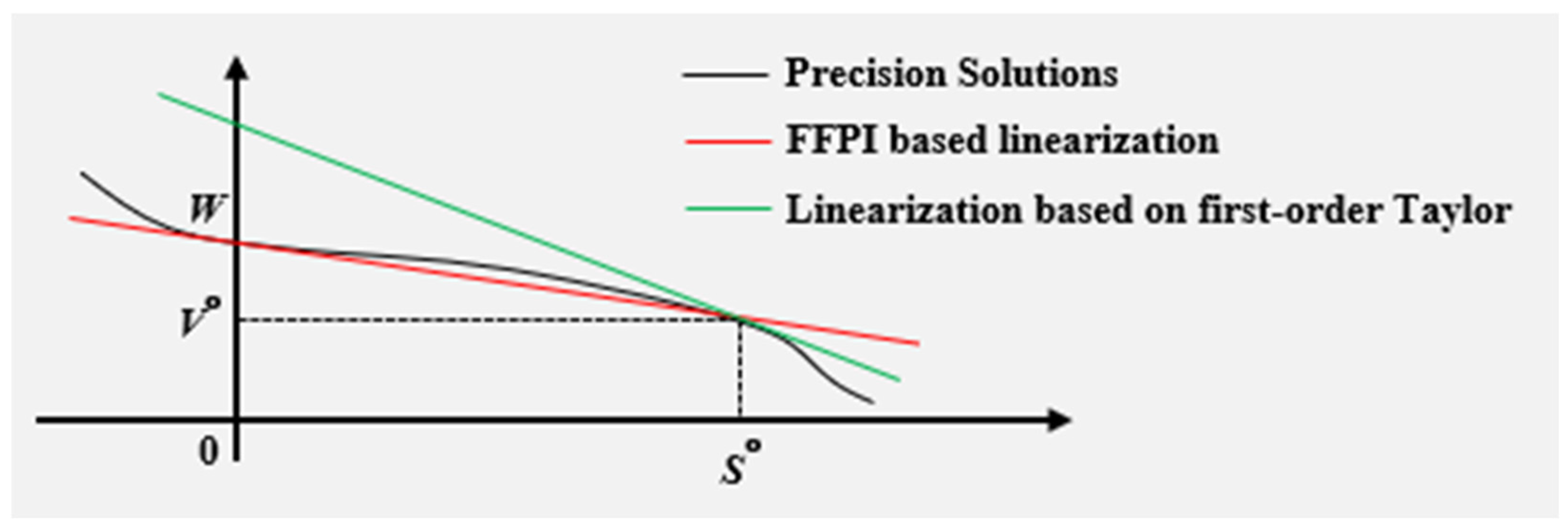
3.2. Zbus Linearized Power Flow Model Based on Fixed-Point Power Iteration

For any nonlinear function y = f(x), when finding its zero x₀, we have f(x₀) = 0. In this case, we can express it in another equivalent form x₀ = Ψ(x₀), where x₀ is the fixed point of the function Ψ(x₀). The actual fixed point is the intersection of the original function and the function y = x. The process of finding the zero of the nonlinear function by computing its fixed point is called fixed-point iteration [21]. The iteration formula is shown in Equation (6) and the iterative process is illustrated in Figure 1.

$$X\left(k\right)=\phi \left(x\right(k-1\left)\right)$$

(6)

From the expression of the Zbus power flow model, it is evident that the Zbus power flow equations exhibit clear iterative function characteristics. It can be proven [22] that for any operating state S⁰ that satisfies the power flow, iteratively calculating the voltage using Equation (6) will converge to the unique solution V⁰. The left-hand side consists of voltages U′ at each PQ node, while the right-hand side represents a function for U′. Therefore, solving these equations can be approached through fixed-point iteration; however, fixed-point iteration typically involves multiple computations and is computationally intensive. Hence, here we adopt the fast fixed-point iteration (FFPI) method based on a single iteration to linearly approximate the Zbus nonlinear model around the reference operating point. In this method, we use the latest operating point U⁰′ as the reference operating point. When there are changes in the power flow in the system, node powers are updated, and according to Equation (7), the node voltages U′ are obtained [2].

$${\mathit{U}}^{\prime }=\mathit{A}{\overline{\mathit{S}}}^{\prime }+\mathit{W}$$

(7)

In the equation $\mathit{A}={{\mathit{Y}}_{LL}}^{-1}\mathrm{d}\mathrm{i}\mathrm{a}\mathrm{g}{\left({\overline{\mathit{U}}}^{\prime 0}\right)}^{-1}$ $\mathit{W}=-{{\mathit{Y}}_{LL}}^{-1}{\mathit{Y}}_{L0}{U}_0$, A and W can be computed offline once the line topology, parameters, and reference operating point are determined. The equation establishes a linear relationship between the node voltages U′ and the injected powers S′ for all nodes in the system, significantly reducing the complexity of the solution process.

The essence of this single fixed-point iteration method is to linearly interpolate between two operating points in the system: (0, W) and (S⁰′, U⁰′). This approach differs fundamentally from standard linearization methods such as tangent-plane approximation at a feasible solution point, such as first-order Taylor expansion. This allows the linear approximation method based on single fixed-point iteration to maintain higher accuracy over a wider range, as illustrated in Figure 2 comparing different linearization methods.

3.3. Voltage Sensitivity Analysis Method

Voltage sensitivity refers to the extent of voltage response in a power system to changes in power (voltage-transfer-limiting process, VTL). Specifically, it measures how changes in power affect node voltages within the power system [23]. By calculating the derivatives of node voltages with respect to factors such as load power changes, generator output power changes, or variations in line parameters, power voltage sensitivity can be obtained. This analysis helps evaluate voltage stability at different nodes in the system, guides grid planning and operations, and determines necessary control measures to ensure the safe and reliable operation of the power system.

Obtaining voltage sensitivity establishes a linear relationship between node voltages and changes in node power, significantly reducing computational complexity. Traditional voltage sensitivity is obtained by inverting the Jacobian matrix, but this method is computationally intensive and impractical for real-time control [23]; moreover, it does not provide sensitivity information about reference nodes; therefore, based on the Zbus power flow model discussed earlier, calculating the partial derivatives of node voltages with respect to injected power yields expressions for voltage sensitivity as shown in Equations (8) and (9). This allows for the quantification of the analytical relationship between node voltages and injected power, thereby greatly reducing computational complexity.

$${\displaystyle \frac{\partial {\mathit{U}}^{\prime }}{\partial \mathit{P}}}={{\mathit{Y}}_{LL}}^{-1}\mathrm{d}\mathrm{i}\mathrm{a}\mathrm{g}{\left({\overline{\mathit{U}}}^{0^{\prime }}\right)}^{-1}$$

(8)

$${\displaystyle \frac{\partial {\mathit{U}}^{\prime }}{\partial \mathit{Q}}}=-j{{\mathit{Y}}_{LL}}^{-1}\mathrm{d}\mathrm{i}\mathrm{a}\mathrm{g}{\left({\overline{\mathit{U}}}^{0^{\prime }}\right)}^{-1}$$

(9)

In the equation, U′ represents the matrix of voltages at each PQ node, P and Q are matrices of active and reactive power at each PQ node, respectively, and U⁰′ denotes the latest operating point of the power flow.

Besides the power injections at each PQ node causing voltage variations, changes in the root node’s voltage also impact the voltages at all nodes. In the ZBus linearized power flow model, the voltages at PQ nodes also exhibit a linear relationship with the voltage vector at the reference node; therefore, based on the linearized power flow equations, derivatives of the reference node voltage U₀ can be computed swiftly, facilitating the rapid calculation of PQ node sensitivity to the reference node voltage. According to the power flow model, the sensitivity of PQ node voltages to the reference node voltage can be solved as shown in Equation (10).

$${\displaystyle \frac{\partial {\mathit{U}}^{\prime }}{\partial U_0}}=-{{\mathit{Y}}_{LL}}^{-1}{\mathit{Y}}_{L0}$$

(10)

The above equation establishes a linear relationship between the voltages of each PQ node and the root node voltage. Using this relationship, it is possible to quantitatively determine how changes in the voltage of the reference node affect the voltages of each PQ node.

In distribution networks, the voltage at each PQ node is primarily influenced by two factors. Firstly, adjustments in the tap position of the OLTC (on-load tap changer) at substations cause changes in the voltage of the reference node, thereby affecting the voltages at each PQ node. Secondly, changes in load power lead to variations in node voltages. Due to the characteristic of distribution network lines having relatively high R/X ratios, there exists a close coupling between voltage and both active and reactive power. In summary, the voltage at each PQ node is related to the voltage at the reference node as well as the active and reactive power at each PQ node. The voltage sensitivity obtained through the Zbus power flow model precisely establishes this linear relationship among these variables. This provides a theoretical basis for calculating voltage regulation boundaries at substations.

4. Day-Ahead Dispatch Optimization Strategy

Before assessing the voltage regulation range of substations, specific data on various state variables within the distribution network must be determined. Based on this foundation, voltage regulation boundaries are computed according to relevant constraints to establish the substation’s voltage regulation range. The primary control method in distribution networks involves adjusting the tap positions of on-load tap changers (OLTCs) to alter the system’s operational state. This study utilizes forecasts of renewable energy and load power values to pre-dispatch adjustments in OLTC tap positions, aiming to minimize network losses throughout the day with optimization intervals set at 15 min. The controlled variable is specifically the OLTC tap position. The day-ahead scheduling optimization model utilizes forecasts of generation sources, load profiles, load power regulation characteristics, and various system parameters as inputs. It aims to optimize network losses by controlling OLTC systems throughout the day, thereby facilitating economic dispatch of the power system.

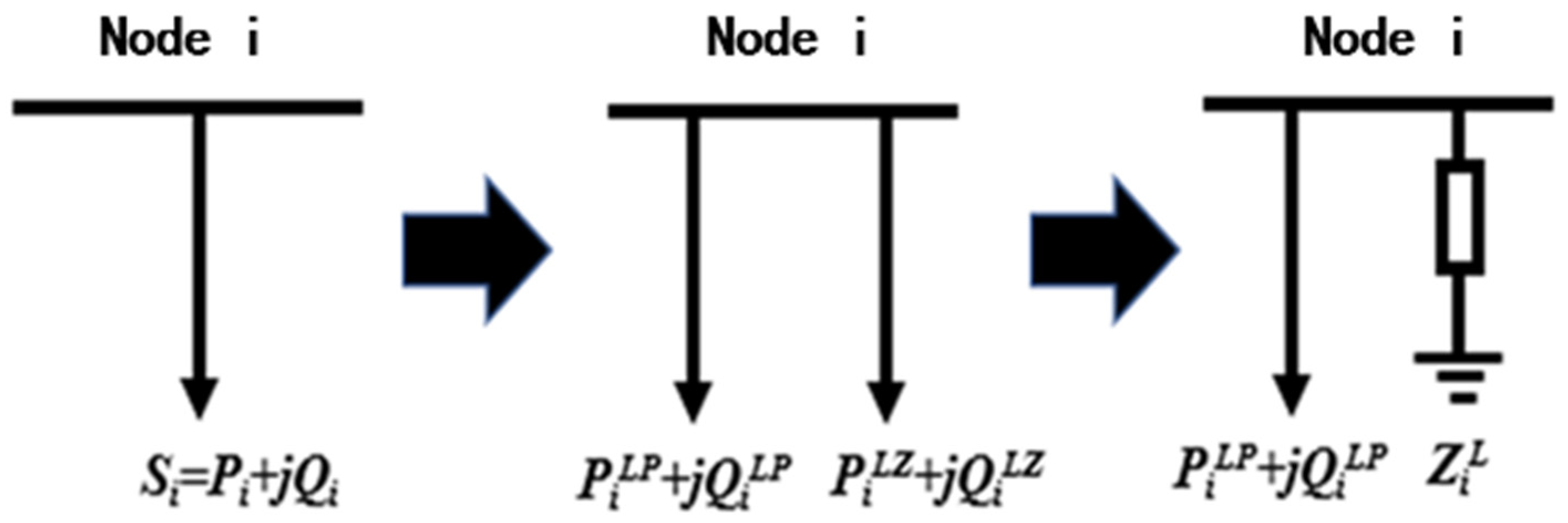
4.1. Considering the Load Active Power–Voltage Coupling Characteristics in the Power Flow Equation Correction

In distribution networks, the loads at various nodes are typically treated as PQ nodes, but in practical distribution systems, there exist varying degrees of coupling between feeder loads and voltage levels. The static characteristics of loads are often represented using a polynomial model known as the ZIP load model, as shown in Equation (11):

$$P_u=P_N\left[A_p{\left({\displaystyle \frac{U}{U_N}}\right)}^2+B_p\left({\displaystyle \frac{U}{U_N}}\right)+C_p\right]$$

(11)

In this equation, Pu represents the active power corresponding to the voltage U; U_N and P_N, respectively, denote the rated voltage and rated power. In Equation (11), the first term is the equivalent constant impedance load, the second term is the equivalent constant current load, and the third term is the equivalent constant power load. Ap, Bp, and Cp represent the proportions of these three types of loads to the total active power load, with Ap + Bp + Cp = 1.

In related research, the ZIP load model is simplified to the ZP load model, as shown in Equation (12):

$$P_u=P_N\left[A_p^{\prime }{\left({\displaystyle \frac{U}{U_N}}\right)}^2+C_p^{\prime }\right]$$

(12)

where Ap′ + Cp′ = 1, differentiation with respect to U = U_N yields an approximation of the load model slope approximately equal to 2 Ap + Bp ≈ 2 Ap′.

In the above load model, the coupling relationship between load power and voltage is verified; however, in distribution networks, feeder load models are typically represented using the voltage reduction energy-saving factor (CVR coefficient), defined as shown in Equation (13). It represents the ratio of the percentage change in active power of the load to the percentage change in voltage. This model characterizes the steady-state regulation characteristics of the load and is commonly used in control applications for feeder loads over medium to long time scales, such as peak shaving and secondary frequency regulation scenarios.

$$CV{R}_f=\Delta P\%/\Delta U\%$$

(13)

From the ZP load model, it is known that when U = U_N, differentiation yields an approximation of the CVR coefficient approximately equal to twice the Ap; therefore, adopting the principle of equivalence, the node load power can be divided into constant power components and constant impedance components based on the CVR coefficient, as shown in Equations (14) and (15):

$$P^{L,P}=C_p{P}^{L,0}=P^{L,0}\left(1-A_P\right)=P^{L,0}\left(1-CV{R}_f/2\right)$$

(14)

$$P^{L,P}=A_p{P}^{L,0}=P^{L,0}\left(CV{R}_f/2\right)$$

(15)

In the equation, P_L,P and P_L,Z, respectively, represent the constant power component and constant impedance component of node active power. For the constant power component, the original Zbus linearization method can be used in the power flow analysis. For the constant impedance component, since its power is proportional to the square of the voltage, it can be represented by the equivalent impedance at the node.

$$Z^L={\left(V^0\right)}^2/\left(P^{L,Z}+j{Q}^{L,Z}\right)$$

(16)

where V₀ is the rated voltage of each node, Z_L is the equivalent impedance of the constant impedance component, and P_L,Z and Q_L,Z are the active and reactive power constant impedance components at the node, respectively.

By using Equations (14)–(16), the node admittance matrix and the power injection matrix of the power flow model can be modified, taking into account the load voltage–power coupling characteristics, as shown in Figure 3.

4.2. Constructing the Objective Function for Minimizing Network Loss

The reactive power optimization problem is a typical optimization issue comprising three main elements: optimization variables, objective function, and constraints. The objective of the current pre-dispatch is to minimize the total network loss throughout the day. Typically, network loss considers only the power losses on each branch; however, this paper modifies the node admittance considering voltage coupling characteristics. Therefore, network loss now includes losses from power dissipation between nodes as well as losses from each node to ground; thus, the objective function expression is as follows:

$$F=min\left(\left.\sum _{i\in N_b}\sum _{t\in T}\left|\Delta P_{lossb i,t}\right|+\sum _{i\in N_{\pi }}\sum _{t\in T}\left|{\Delta P}_{lossn i,t}\right|\right)\right.$$

(17)

In the equations, P_{lossb i,t} represents the network loss on branch i during time period t. P_{lossn i,t} represents the network loss of node i to ground during time period t. T is the set of all time periods in a day. N_b is the set of distribution network branches. The objective function is related to minimizing the total system-wide network loss over the entire day. Due to varying power levels of renewable energy sources and loads across different time periods, the network losses on distribution branches also vary. Generally, higher voltage levels correspond to lower power losses on branches (the first term in the equation), while losses from nodes to ground increase with higher voltage levels (the second term). The core objective is to determine appropriate OLTC (on-load tap changer) positions to minimize the sum of daily network losses in the system.

4.3. Modeling Constraint Conditions

(1) Node Voltage Constraints

In distribution networks, the reactance of the lines is relatively small, therefore node voltage constraints can be approximated using voltage magnitudes, as shown in Equation (18):

$$V_{imin}\le V_i\left(k\right)\le V_{imax}$$

(18)

Here, Vi(k) represents the voltage magnitude of node i at time k and V_imin and V_imax are the lower and upper limits of the voltage at node i, respectively. These limits denote the allowable voltage range for the safe operation of the distribution network, with values of 0.93 p.u. and 1.07 p.u.

(2) Voltage regulation device operational constraints

On-load tap changer (OLTC): OLTCs are typically installed at the beginning of a line and can adjust the system voltage at the connection point as a whole, offering high control efficiency. When using OLTCs to regulate voltage, the output voltage depends on their operating tap position, and there is a need to limit the number of tap changes per day.

$$V_{i,t}^{\mathrm{out}}=V_{i,t}^{in}+X_{i,t}^{OLTC}{V}_{\mathrm{tap}}\hspace{1em}\forall i\in {\mathit{N}}_{\mathit{O}\mathit{L}\mathit{T}\mathit{C}},t\in \mathit{T}$$

(19)

$$X_{i min}^{OLTC}\le X_{i,t}^{OLTC}\le X_{i max}^{OLTC}\hspace{1em}\forall i\in {\mathit{N}}_{OLTC}$$

(20)

$$\sum _{t\in T} \left|{X_{i,t}}^{{ }^{OLTC}}-{X_{i,t-1}}^{{ }^{OLTC}}\right|\le {N_{max}}^{OLTC} \forall i\in {\mathit{N}}_{OLTC}$$

(21)

In the formula, V_{i, t}^out and V_{i, t}ⁱⁿ represent the output voltage of the OLTC before and after tap adjustments, respectively, for node i. X_{i, t}^OLTC denotes the tap position of the OLTC at node i during time interval t. Vtap represents the voltage change per tap position of the OLTC. X_imin^OLTC and X_imax^OLTC are the lower and upper limits of the tap positions for the OLTC at node i, respectively. N_max^OLTC is the maximum allowable number of tap changes per day for the OLTC. N_OLTC denotes the set of nodes where the OLTC is installed.

5. Methods for Assessing Voltage Regulation Range at Substations

Based on the optimization through day-ahead scheduling, the state parameters of OLTCs, new energy inverters, circuit breakers (CBs), SVCs, and other voltage regulation devices are predetermined. Utilizing this foundation along with day-ahead forecasts of generation and load information, voltage sensitivity analysis is employed to evaluate the margin for tap adjustment at OLTCs in substations. Considering the reactive power compensation capabilities within the network, voltage conditions at nodes within the range of reactive power compensation are calculated using analytical voltage sensitivity. Ensuring overall grid voltage security, the objective is to maximize the active power regulation capacity of substations by determining their adjustable capacity. The process of tap adjustments causing changes in balanced node voltages and thereby affecting the voltages of various PQ nodes can be linearly represented using expressions for balanced node voltage sensitivity. Adjustments in reactive power injection caused by capacitors (CBs), Static Var Compensators (SVCs), photovoltaic, wind inverters, and other reactive power regulation devices influencing node voltage changes can be linearly expressed through reactive power–voltage sensitivity; therefore, based on analytical voltage sensitivity and considering relevant constraints, assessment of voltage regulation range at substations can be conducted.

5.1. Constructing an Optimization Objective Function

The on-load tap-changing transformers in medium-voltage substations possess strong voltage regulation capabilities, allowing them to raise or lower the distribution network voltage from the root node; therefore, when considering them as the adjustment target for substation load control, it is essential to ensure the safety of network node voltages. Consequently, the objective function is initially formulated to maximize the voltage regulation range of the medium-voltage substation; on the other hand, optimization calculations are performed separately for scenarios involving maximum voltage raise and maximum voltage drop, while minimizing reactive power compensation adjustments to ensure continuous control margins. Two specific objective functions are defined for online capacity assessment, expressed as follows:

$$F_1=max\left({\alpha }_1\left(k_1-k_{0,t}\right)\Delta V_{\mathrm{tap} }-{\alpha }_2\sum _{i=1}^M \left|\Delta Q_i\right|\right)$$

(22)

$$F_2=max\left({\alpha }_1\left(k_{0,t}-k_2\right)\Delta V_{\mathrm{tap} }-{\alpha }_2\sum _{i=1}^M \left|\Delta Q_i\right|\right)$$

(23)

In the two objective functions, ΔV_tap represents the voltage adjustment step of the on-load tap changer, which is the voltage change corresponding to one tap position change. k_0,t, k₁, and k₂, respectively, denote the current tap position at time t, the tap position maximizing the capacity for upward adjustment, and the tap position maximizing the capacity for downward adjustment. ΔQ_i is the reactive power compensation adjustment of device i, and α₁ and α₂ are weighting coefficients.

In the objective functions, the first part aims to maximize the range of voltage adjustment either upwards or downwards, while the second part aims to minimize the network’s reactive power compensation adjustment. Due to the discrete nature of OLTC adjustment, once the reactive power compensation adjustment reaches a certain level, further changes in reactive power under relevant constraint conditions cannot expand the voltage adjustment range further.

5.2. Modeling Constraint Conditions

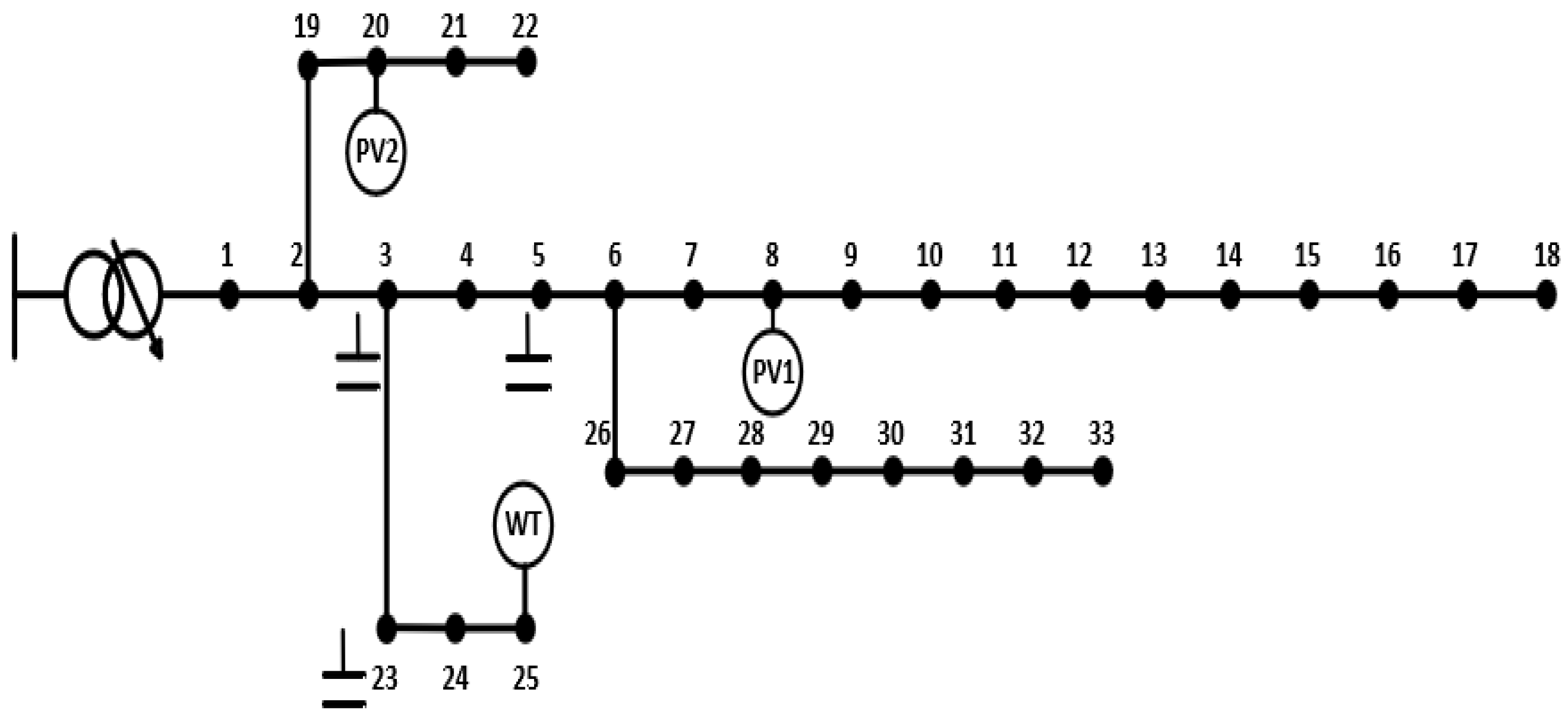
This paper is based on analytical voltage sensitivity to rapidly calculate the impact of on-load tap changers on network voltage. It also considers the influence of controllable reactive power compensation within the system on node voltages to ensure maximum adjustability of substation load capacity; therefore, various operational constraints of adjustable resources and voltage safety constraints are taken into account.

(1) Node Voltage Constraints

In distribution networks, the reactance of the lines is relatively small, hence node voltage constraints can be approximated using voltage magnitudes, as shown in Equation (24):

$$V_{imin}\le V_i\left(k\right)\le V_{imax}$$

(24)

Here, Vi(k) represents the voltage magnitude of node i at time k and V_imin and V_imax are the lower and upper limits of the voltage at node i, respectively. These limits denote the allowable voltage range for the safe operation of the distribution network, with values of 0.93 p.u. and 1.07 p.u.

(2) Voltage Regulation Device Operational Constraints

On-load Tap-Changing Device (OLTC): Same as Section 4.3

Photovoltaic (PV) Equipment: Photovoltaic systems generate electricity by harnessing solar energy. They can adjust their inverters to provide or absorb a certain amount of reactive power as needed, assisting in voltage regulation of the grid. PV reactive power control strategies mainly include PQ control and PV control. In the PQ control mode, PV devices provide a fixed amount of reactive power as instructed, maintaining the specified power output regardless of changes in grid conditions. This ensures that the grid’s power requirements are met and reactive power support is provided. In the PV control mode, PV devices adjust their active power output based on changes in grid voltage to keep the grid voltage stable within a set range. This enhances grid voltage quality and stability, although fundamentally it still involves reactive power control. The choice between these control types depends on grid requirements and the design goals of the PV system, aiming to effectively regulate and support the grid.

$$Q_i^{PVmin}\le {Q_{i,t}}^{PV}\le Q_i^{PVmax}\hspace{1em}\forall i\in {\mathit{N}}_{PV},t\in \mathit{T}$$

(25)

$$\left|{Q_{i,t}}^{PV}\right|\le \sqrt{{\left(S_i^{PV}\right)}^2-{\left({P_{i,t}}^{PV}\right)}^2}\hspace{1em}\forall i\in {\mathit{N}}_{PV},t\in \mathit{T}$$

(26)

$$V_{P{V}_{min}}\le V_{i,t}\le V_{PVmax}\hspace{1em}\forall i\in {\mathit{N}}_{PV},t\in \mathit{T}$$

(27)

$$P_{i,t}^{PV}=P_{i,t}^{PV pre } \forall i\in {\mathit{N}}_{PV},t\in \mathit{T}$$

(28)

The output power of PQ-type photovoltaics is subject to certain constraints. In addition to output power, PV-type photovoltaics also need to restrict the voltage level at the grid connection point. In the equations, P_i,t^PV and Q_i,t^PV, respectively, denote the active and reactive powers of the i-th node in the photovoltaic system during time period t; Q_i^PVmax and Q_i^PVmin are the maximum and minimum reactive power values of the i-th node in the photovoltaic system; S_i^PV is the rated capacity of node i in the photovoltaic system; V_i,t represents the grid voltage at node i of the photovoltaic system during time period t; V_PVmax and V_PVmin are, respectively, the maximum and minimum e values at the photovoltaic grid connection point; P_i,t^PV Pre is the predicted active power of node i’s photovoltaic system during time period t; N_PV represents the collection of photovoltaic nodes.

Wind turbine equipment: The operation modes are also divided into PQ control and PV control, and the operational constraints are similar to photovoltaic devices.

$$Q_i^{WTmin}\le {Q_{i,t}}^{WT}\le Q_i^{WTmax}\hspace{1em}\forall i\in {\mathit{N}}_{WT},t\in \mathit{T}$$

(29)

$$\left|{Q_{i,t}}^{WT}\right|\le \sqrt{{\left(S_i^{WT}\right)}^2-{\left({P_{i,t}}^{WT}\right)}^2}\hspace{1em}\forall i\in {\mathit{N}}_{WT},t\in \mathit{T}$$

(30)

$$V_{WT}\le V_{i,t}\le V_{WTmax}\hspace{1em}\forall i\in {\mathit{N}}_{WT},t\in \mathit{T}$$

(31)

$$P_{i,t}^{WT}=P_{i,t}^{WT pre } \forall i\in {\mathit{N}}_{WT},t\in \mathit{T}$$

(32)

In the equations, P_i,t^WT and Q_i,t^WT, respectively, denote the active and reactive power of the i-th node in the wind turbine system during time period t; Q_i^WTmax and Q_i^WTmin are the maximum and minimum reactive power values of the i-th node in the wind turbine system; S_i^WT is the rated capacity of node i in the wind turbine system; V_i,t represents the grid voltage at node i of the wind turbine system during time period t; V_WTmax and V_WTmin are, respectively, the maximum and minimum grid voltage values at the wind turbine grid connection point; P_i,t^{WT Pre} is the predicted active power of node i’s wind turbine system during time period t; and N_WT represents the collection of wind turbine nodes.

Capacitor Bank (CB) equipment: Capacitor banks are commonly used reactive power compensation devices in electrical power systems, typically employed to improve power factors and optimize voltage regulation. They consist of multiple capacitor units connected in parallel or series configurations to provide the required capacity and performance. Compared to other reactive power compensation devices, capacitor banks have limitations on the number of switching operations they can undergo.

$${Q_{i,t}}^{CB}={X_{i,t}}^{CB}{Q_i}^{CBR}\hspace{1em}\forall i\in {\mathit{N}}_{CB},t\in \mathit{T}$$

(33)

$$\sum _{t\in T}\left|{X_{i,t}}^{CB}-{X_{i,t-1}}^{CB}\right|\le {N_{max}}^{CB}\hspace{1em}\forall i\in {\mathit{N}}_{\mathit{C}\mathit{B}}$$

(34)

In the equation, Q_i^CBR represents the rated capacity of the shunt capacitor bank connected to node i; X_i,t^CB denotes the switching state of the capacitor bank group, where X_i,t^CB = 1 when the capacitor bank group is in operation, and during this period, the reactive power Q_i,t^CB injected by the capacitor bank group at node i is Q_i^CBR. Conversely, X_i,t^CB = 0 indicates that the capacitor bank is not in operation, thus Q_i,t^CB = 0. N_max^CB is the daily threshold for the maximum number of switching operations for the capacitor bank; N_CB represents the set of nodes where capacitor banks are installed.

Static Var Compensator (SVC) Device: SVC reactive power compensation has upper and lower limits, specified as follows:

$$Q_i^{SVCmin}\le Q_{i,t}^{SVC}\le Q_i^{SVC}\max \hspace{1em}\forall i\in N_{SVC},t\in T$$

(35)

In the equation, Q_i,t^SVC represents the reactive power of SVC at node i during time period t; Q_i^SVCmax and Q_i^SVCmin denote the maximum and minimum values of reactive power for SVC at node i, respectively; N_SVC represents the set of nodes where SVCs are installed.

(3) Voltage Variation Constraints

Based on the analytical results from voltage sensitivity calculations, node voltages can be computed rapidly.

$$\Delta \mathit{V}={\displaystyle \frac{\partial \mathit{V}}{\partial V_0}}\Delta V_t^{\mathrm{OLTC} }+{\displaystyle \frac{\partial \mathit{V}}{\partial \mathit{Q}}}\Delta {\mathit{Q}}_t$$

(36)

In the equation, ∂V/∂Q and ΔQ, respectively, denote the sensitivity of node voltage to changes in reactive power injection at the node, and the current reactive power compensation variation at the same time. ΔV represents the vector composed of voltage changes at each node.

Based on the above, the overall analysis process for OLTC (on-load tap changer) voltage regulation range assessment is illustrated in Figure 4.

6. Case Analysis

In this section, a distribution network system is constructed using the MATLAB simulation platform, with a topology structure depicted in Figure 5. The model utilizes an enhanced IEEE 33-node system [24]. The system begins with a tap changer device at the primary end to simulate the OLTC (on-load tap changer) inside a substation. The nominal voltages are 110 kV on the high-voltage side and 10 kV on the low-voltage side. Node 1 serves as the balanced node, while the remaining nodes are PQ nodes. The total system load is 3715 kW + j2300 kvar. The system includes three distributed renewable energy sources: PV1 and PV2 are PQ-controlled photovoltaic units connected to nodes 8 and 20, respectively, each with a rated capacity of 1000 kW; WT is a PQ-type wind turbine connected to node 24 with a rated capacity of 800 kW. The total installed capacity of renewable energy sources is 2200 kW (0.22 pu), resulting in a renewable energy penetration rate of 75.4%. Additionally, the system incorporates three switchable capacitor banks CB1, CB2, and CB3 connected to nodes 3, 5, and 23, respectively, each with a rated capacity of 300 kvar.

The model only includes absolute value terms in the objective function, making it easier to linearize. After steps such as linearizing power flows and conducting sensitivity analysis on voltages, the entire model becomes linear. It is treated as a Mixed-Integer Linear Programming (MILP) problem and directly solved using the GUROBI solver on the MATLAB platform for rapid solution.

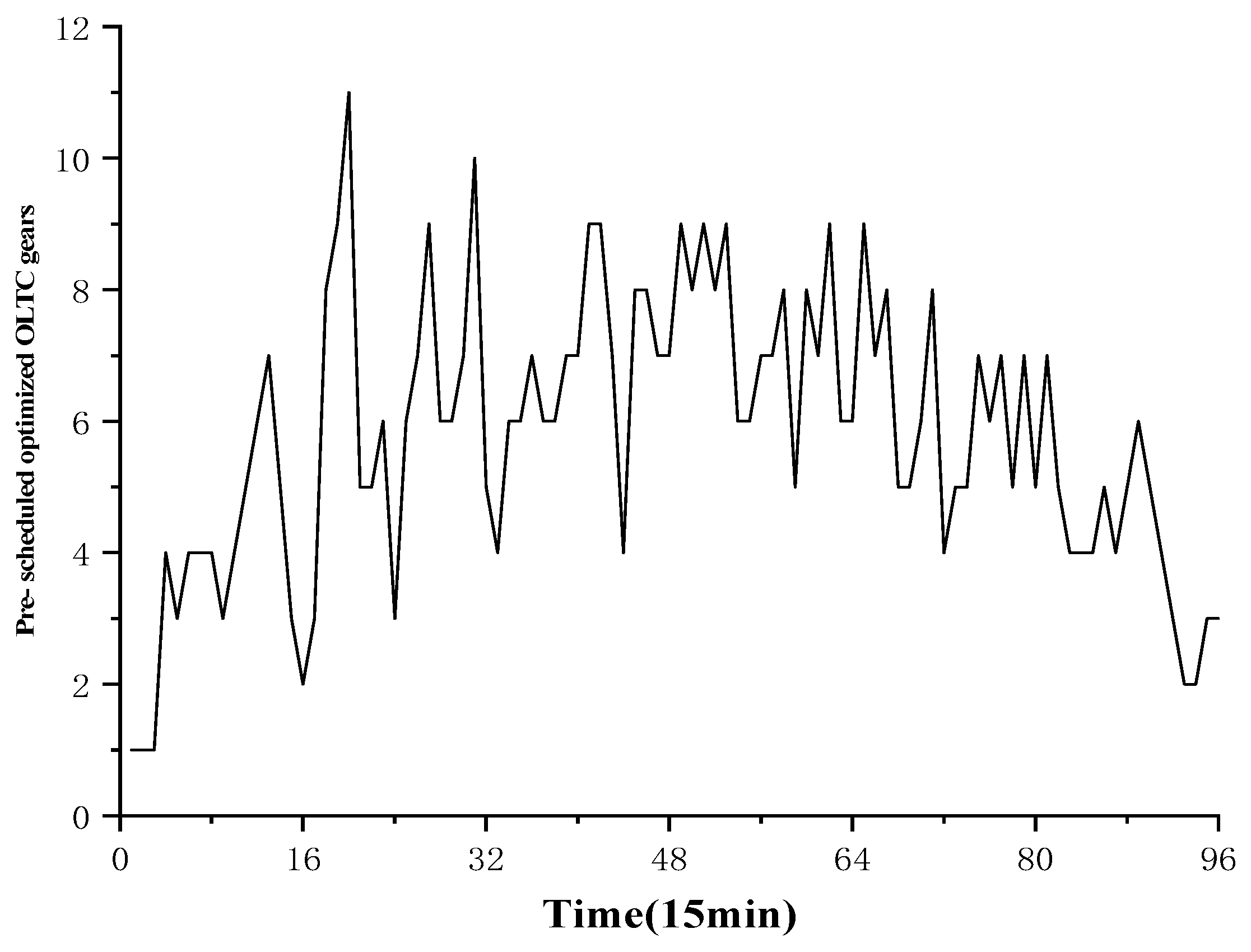
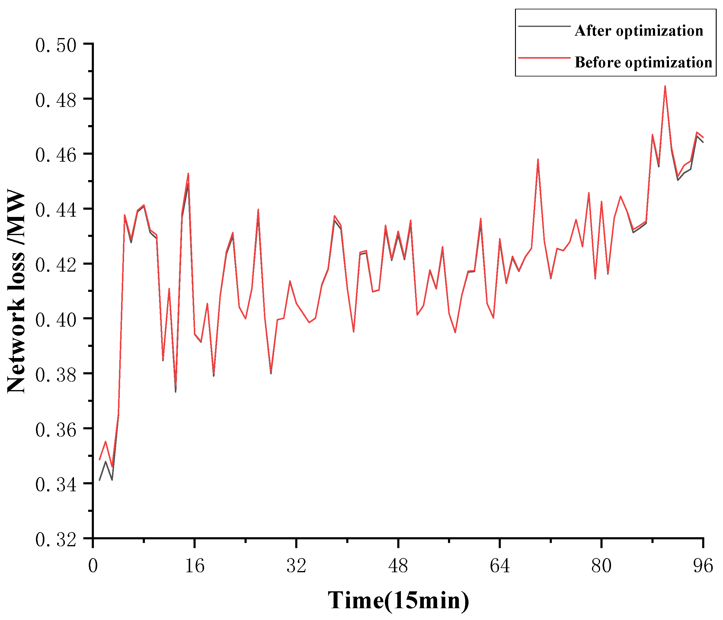
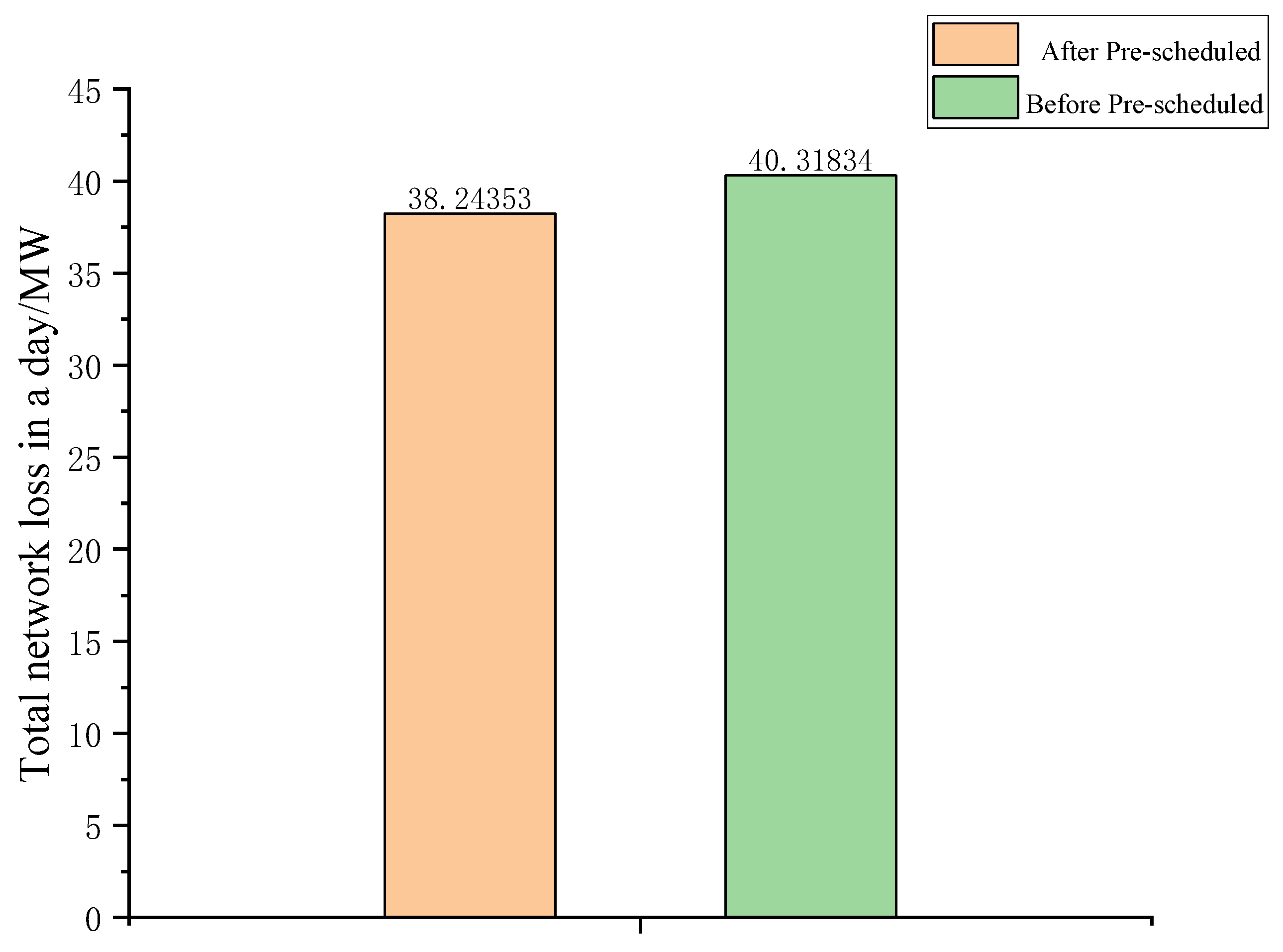
6.1. Day-Ahead Dispatching Results

Based on the hypothesized source-load prediction curves and system operating parameters, optimal power flow calculations with the objective of minimizing network losses are conducted using the GUROBI solver. This process determines the appropriate OLTC (on-load tap changer) tap setting to ensure minimal power losses across the entire network. It is assumed that the transformer has 11 tap positions, from 1 to 11, with each tap adjustment being 0.0125 p.u. The pre-scheduling optimization interval is 15 min, and this case study uses a 24 h optimization period. The optimization results are shown in Figure 6, where the x-axis represents time, with each optimization occurring every 15 min, and numbers 0–96 correspond to the sequence of optimization instances. Additionally, a comparison example with the OLTC always set to the middle tap position is provided, with results shown in Figure 7 and Figure 8. Figure 7 presents a line chart comparing the results of each optimization, while Figure 8 compares the total network losses before and after optimization within one day using a bar chart.

According to the analysis results from Figure 7 and Figure 8, although there is no significant change in network loss before (with OLTC set at the middle tap position of 1.0 p.u.) and after optimization, the network loss after each pre-scheduling optimization is generally lower than that before optimization; additionally, the total network loss within a day notably decreases, confirming the effectiveness of the optimization strategy. Typically, power losses in branches between nodes decrease as voltage levels increase; however, due to the power–voltage coupling characteristics of distribution network feeder loads, it is necessary to introduce grounded impedance branches to describe this characteristic. The power losses in equivalent grounded branches increase with higher voltage levels, which is opposite to the situation with node branches; therefore, by selecting appropriate OLTC tap positions to ensure proper voltage levels, the overall network losses of the system can be effectively reduced.

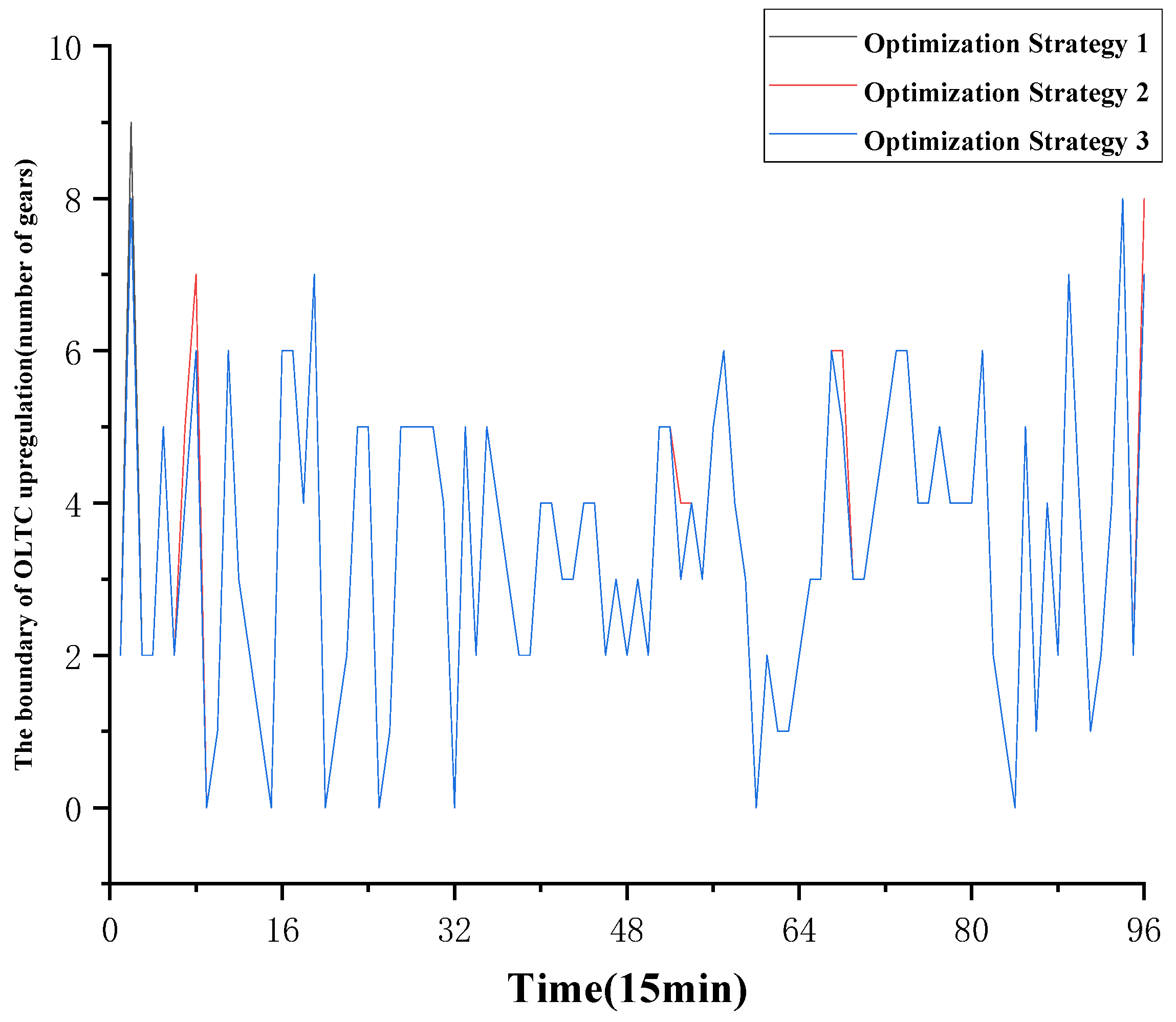
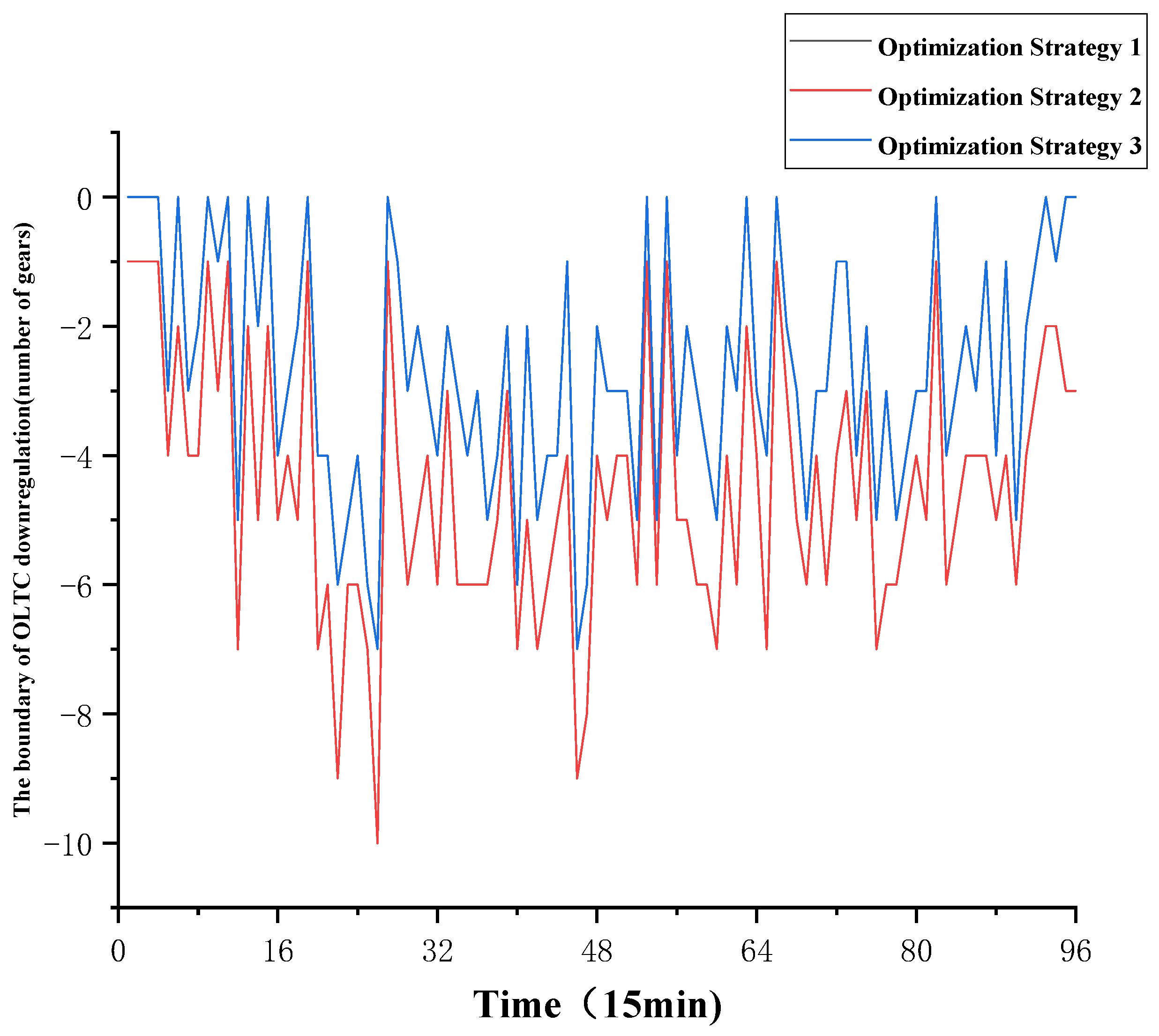
6.2. Intraday Tap Range Calculation

The intraday optimization interval is also 15 min, with a duration of 24 h. Based on real-time measurements of resources and network status, the transformer tap voltage adjustment boundaries are computed for each period within a day. Analysis is conducted under scenarios considering only the first term of the objective function and both terms. This examines the boundaries of transformer adjustments and the total reactive power injection.

Optimization Strategy 1: only maximize the voltage adjustment boundaries by setting the weighting coefficients α1 and α2 of the objective function to 1 and 0, respectively.

Optimization Strategy 2: Aim to increase the tap voltage adjustment range while minimizing reactive power compensation adjustments. Set the weighting coefficients α1 and α2 of the objective function to 1 and 0.9, respectively.

Optimization Strategy 3: Aim to increase the tap voltage adjustment range while simultaneously minimizing reactive power compensation adjustments. Set the weighting coefficients α1 and α2 of the objective function to 0.5 and 0.5, respectively.

Using the MATLAB simulation platform with the GUROBI solver for optimization, the upper and lower bounds of OLTC adjustments are shown in Figure 9 and Figure 10.

Observing Figure 9 and Figure 10, based on the pre-scheduled OLTC optimization results, it is evident that the adjustment boundary curves for Optimization Strategy 1 and Optimization Strategy 2 completely overlap and are noticeably higher than those for Optimization Strategy 3. This is because when the weight coefficient of the second term in the objective function is set higher, the optimization process may focus on minimizing the total reactive power compensation, which can prevent maximizing the voltage adjustment range and potentially result in smaller OLTC adjustment boundaries. Comparing the adjustment boundary curves between Optimization Strategy 1 and Optimization Strategy 2 reveals that with appropriately set weight coefficients, there is little to no impact on the voltage adjustment range.

The three curves for the upper tap boundaries of OLTC almost overlap. This is typically because the root node voltage is usually the highest, and during the adjustment process, the root node may exceed limits first. The reactive power compensation devices below the substation have minimal impact on the root node voltage, thus these devices remain largely inactive.

The total reactive power compensation during the adjustment process is illustrated in Figure 11 and Figure 12.

From Figure 11, it can be observed that for most periods, the total reactive power compensation for all three optimization strategies is zero. This is also due to the fact that during the tap increase process, the root node voltage exceeds limits first, and the reactive power compensation devices below the substation cannot affect the voltage at the root node. In a few periods, however, due to the initial reactive power injection, some nodes on the feeder may have voltages higher than the root node, resulting in non-zero reactive power compensation.

From the data in Figure 12, it can be seen that during downward adjustments, the adjustment boundaries for Optimization Strategy 1 and Strategy 2 are identical across all optimization intervals; however, the total reactive power adjustment for Strategy 2 is consistently lower than that for Strategy 1. Figure 13 shows that Strategies 2 and 3 both have significantly lower total reactive power adjustments within a day compared to Strategy 1. Although Strategy 3’s total reactive power adjustment is slightly higher than Strategy 2’s, Figure 10 and Figure 11 reveal that Strategy 3 has a narrower voltage adjustment range; therefore, Strategy 2’s results are closest to the expected optimization goals, indicating that appropriately setting the weight coefficients of the objective function can maximize the voltage adjustment range while minimizing the total reactive power adjustment and economic costs.

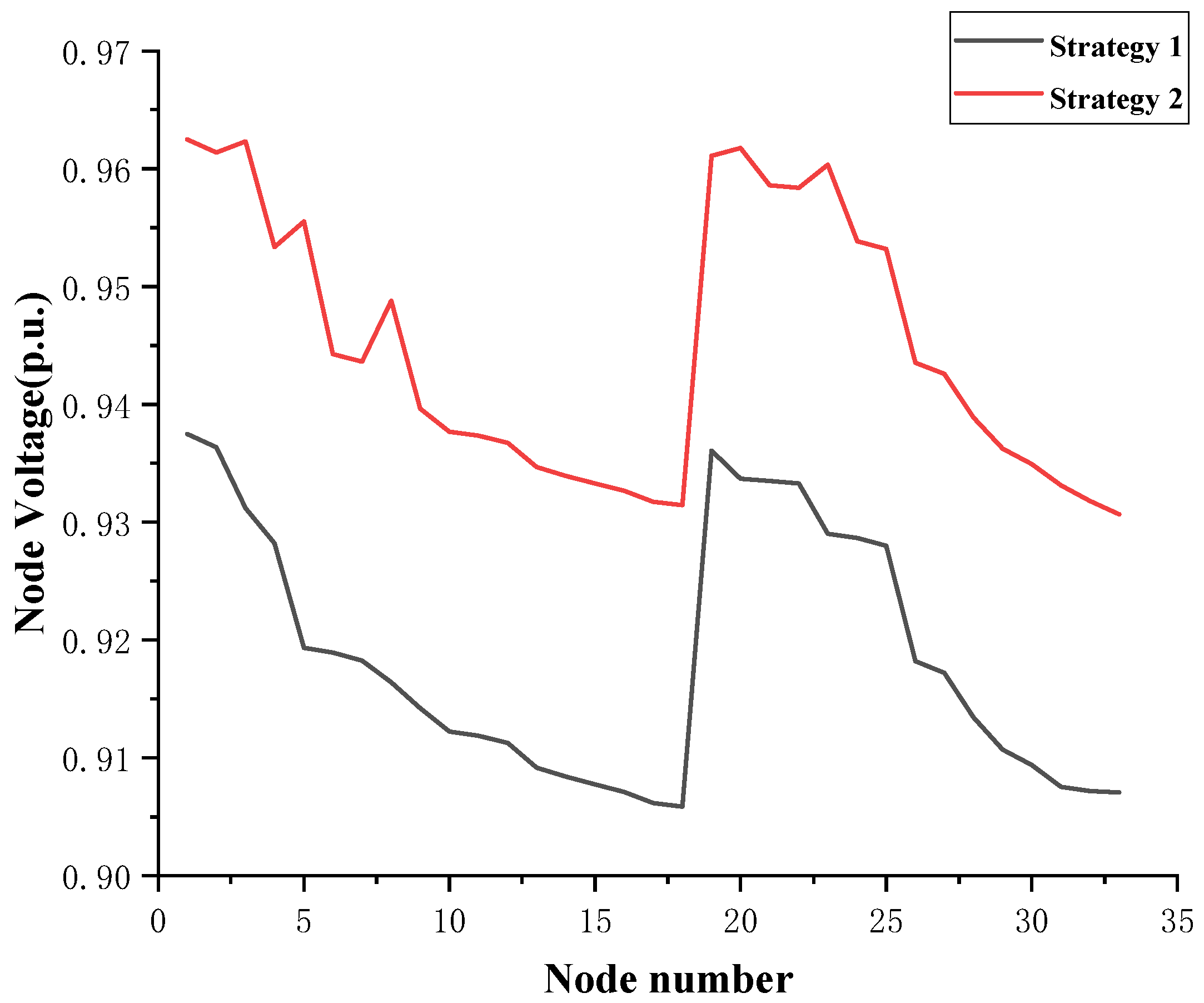
6.3. Analysis of Voltage Exceeding Limits

In traditional studies, the voltage adjustment range for medium-voltage substations is often simply considered to be 0.93 p.u. to 1.07 p.u. However, in practical voltage control, for example in a 110 kV substation, reducing the voltage may lead to voltage violations at various nodes along the feeders; therefore, using the traditional default voltage adjustment range of 0.93 p.u. to 1.07 p.u. as a comparison case, the voltage fluctuations and violations at each node under two strategies are analyzed. Given the extended time period in the example, only a specific time snapshot is analyzed. Based on Section 6.1 and Section 6.2, results from the 48th optimization interval are analyzed, where the root node voltage is lowered to the corresponding strategy’s allowable minimum and the voltage violations at each node are examined. The results are shown in Figure 14.

Strategy 1 assumes the allowable voltage fluctuation range for medium-voltage substations is 1.0 p.u. ± 0.07 p.u.

Strategy 2 uses the method proposed in this paper to evaluate the adjustable voltage range of the medium-voltage substation, considering the reactive power compensation devices and voltage constraints at each node.

From the data in Figure 14, it can be seen that when the substation voltage is adjusted based on the adjustment boundaries calculated using the traditional method, the voltage at most load nodes on the feeders falls below 0.93 p.u., leading to a decrease in voltage quality and the safety operating conditions of the grid not being met. In contrast, when adjusting based on the adjustable range derived from Strategy 2, no node voltage exceeds its limits. This allows for the maximum voltage adjustment range at the medium-voltage substation while ensuring the safe operation of the distribution network.

7. Conclusions

Clarifying the adjustable range of on-load tap changers (OLTCs) and corresponding voltage levels at medium-voltage substations is crucial for enabling load-side resources to participate in grid control. This paper proposes an assessment method for the voltage adjustment range of medium-voltage substations based on analytical voltage sensitivity. The main contributions include the following:

• Development of a Linearized Power Flow Model: A Zbus linearized power flow model based on fixed-point iteration is established and an analytical voltage sensitivity expression is derived from this model. This model establishes a linear relationship between node voltages, node powers, and the root node voltage, clarifying the impact of adjusting the root node voltage and reactive power on the voltages of each PQ node.
• Pre-Scheduling Optimization: In the day-ahead stage, an OLTC pre-scheduling model is constructed based on resource and network state forecasts. This optimization model targets the tap positions as optimization variables and aims to minimize network losses.
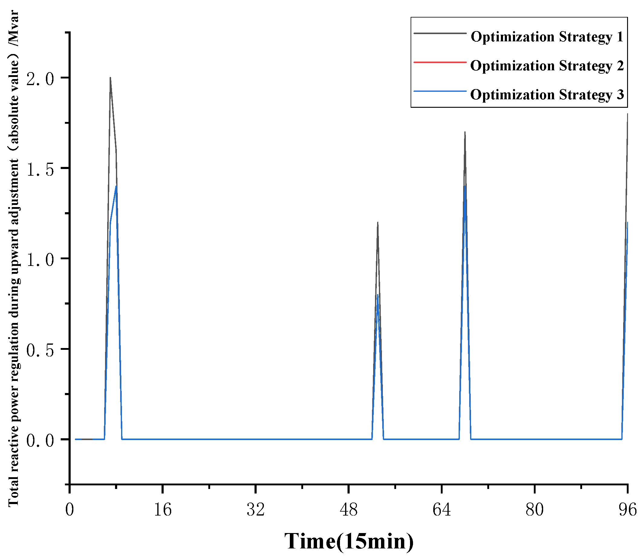
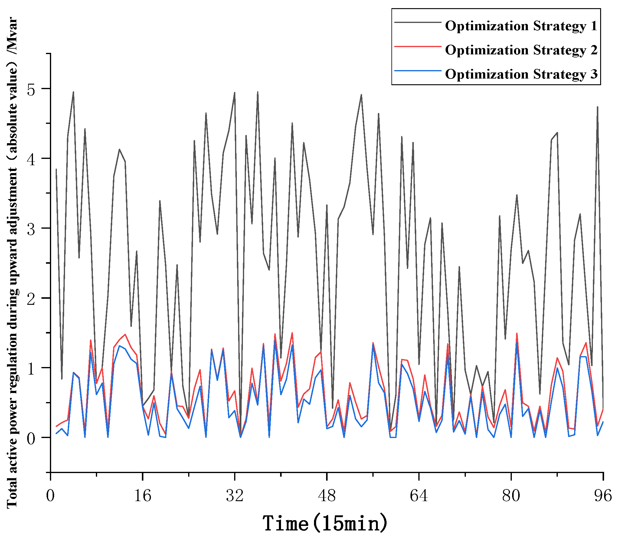
• Real-Time Optimization: In the intraday stage, reactive power control devices such as photovoltaic inverters, SVCs, and circuit breakers are optimized. The goal is to maximize the voltage adjustment range of the medium-voltage substation while minimizing the total reactive power adjustment. This provides boundary conditions for grid control commands.

Due to the limitations of OLTCs (discrete adjustment), the proposed correction strategy only identifies the CVR (Conservation Voltage Reduction) coefficient for the entire substation and does not delve into each feeder or node. Identifying and continuously updating the CVR coefficients for each load node could enable real-time corrections to the admittance matrix and node power injection matrix, resulting in more accurate power flow analysis; additionally, because OLTCs provide discrete voltage adjustments with lower precision, it may not fully utilize the adjustable capacity of feeder loads; therefore, introducing more precise continuous adjustment devices could enhance the voltage adjustment range of medium-voltage substations.

References

1. Han, T.; Gao, Z.; Du, W.; Hu, S. Multi-dimensional evaluation method for new power system. Energy Rep. 2022, 8, 618–635. [Google Scholar] [CrossRef]
2. Boyu, X.I.E. Study on the Peaking and Power Fluctuation Smoothing Strategy of High-Proportion New Energy Distribution Grid Based on Feeder Load Power Control. Ph.D. Thesis, Wuhan University, Wuhan, China, 2022. [Google Scholar]
3. Hou, J.; Yu, W.; Xu, Z.; Ge, Q.; Li, Z.; Meng, Y. Multi-time scale optimization scheduling of microgrid considering source and load uncertainty. Electr. Power Syst. Res. 2023, 216, 109037. [Google Scholar] [CrossRef]
4. Yang, M.; Wang, T.; Wang, Z.B. Considering dynamic perception of fluctuation trend for long-foresight-term wind power prediction. Energy 2024, 289, 130016.1–130016.11. [Google Scholar] [CrossRef]
5. Wu, Y.F.; Liu, H.T.; Xiao, Z.F. Review of incremental distribution network planning considering the uncertainty of source-network-load. Power Syst. Prot. Control. 2021, 49, 177–187. [Google Scholar]
6. Mosca, C.; Arrigo, F.; Mazza, A.; Bompard, E.; Carpaneto, E.; Chicco, G.; Cuccia, P. Mitigation of frequency stability issues in low inertia power systems using synchronous compensators and battery energy storage systems. IET Gener. Transm. Distrib. 2019, 13, 3951–3959. [Google Scholar] [CrossRef]
7. Tian, S.M.; Wang, B.B.; Zhang, J. Key Technologies for Demand Response in Smart Grid. Proc. CSEE 2014, 34, 3576–3589. [Google Scholar]
8. Xu, J.; Cao, H.Q.; Tang, C.H.; Wei, C.; Jiang, H.; Liao, S. Optimal Dispatch of Power System Considering Uncertainty of Demand Response Based on Extended Sequence Operation. Autom. Electr. Power Syst. 2018, 42, 152–160. [Google Scholar]
9. Hosseini, Z.S.; Khodaei, A.; Fan, W.; Hossan, M.S.; Zheng, H.; Fard, S.A.; Paaso, A.; Bahramirad, S. Conservation voltage reduction and volt-var optimization: Measurement and verification benchmarking. IEEE Access 2020, 8, 50755–50770. [Google Scholar] [CrossRef]
10. Han, B.M.; Choi, N.S.; Lee, J.Y. New Bidirectional Intelligent Semiconductor Transformer for Smart Grid Application. IEEE Trans. Power Electron. 2014, 29, 4058–4066. [Google Scholar] [CrossRef]
11. Ghosh, A.; Ledwich, G. Compensation of distribution system voltage using DVR. IEEE Trans. Power Deliv. 2002, 17, 1030–1036. [Google Scholar] [CrossRef]
12. Ding, M.; Wang, W.S.; Wang, X.L.; Song, Y.T.; Chen, D.Z.; Sun, M. A Review on the Effect of Large-scale PV Generation on Power Systems. Proc. CSEE 2014, 34, 1–14. [Google Scholar]
13. Chen, W.J.; Gan, W.; Zhang, J.; Shen, C.; Lin, C.; Wu, M.; Sun, L.; Gu, W.; Zhang, R.; Yang, L.; et al. Divisional and Hierarchical Voltage Regulation Strategy Based on HEM Sensitivity for Distribution Network. Electr. Power Constr. 2022, 43, 42–52. [Google Scholar]
14. Samadi, A.; Eriksson, R.; Söder, L.; Rawn, B.G.; Boemer, J.C. Coordinated Active Power-Dependent Voltage Regulation in Distribution Grids With PV Systems. IEEE Trans. Power Delivery. 2014, 29, 1454–1464. [Google Scholar] [CrossRef]
15. Feng, Y.; Li, Y.; Cao, Y.; Zhou, Y. Automatic voltage control based on adaptive zone-division for active distribution system. In Proceedings of the 2016 IEEE PES Asia-Pacific Power and Energy Engineering Conference (APPEEC), Xi’an, China, 25–28 October 2016; pp. 278–282. [Google Scholar]
16. Ku, T.; Lin, C.; Chen, C.; Hsu, C.T.; Hsieh, W.L.; Hsieh, S.C. Coordination of PV Inverters to Mitigate Voltage Violation for Load Transfer Between Distribution Feeders With High Penetration of PV Installation. IEEE Trans. Ind. Appl. 2016, 52, 1167–1174. [Google Scholar] [CrossRef]
17. GB/T 12325-2008; Power Quality-Deviation of Supply Voltage. Standardization Administration of China: Beijing, China, 2008.
18. Mccarthy, C.; Josken, J. Applying capacitors to maximize benefits of conservation voltage reduction. In Proceedings of the IEEE Rural Electric Power Conference, Raleigh, NC, USA, 4–6 May 2003; pp. C4-1–C4-5. [Google Scholar]
19. Kulworawanichpong, T. Simplified Newton–Raphson power-flow solution method. Int. J. Electr. Power Energy Syst. 2010, 32, 551–558. [Google Scholar] [CrossRef]
20. Mu, S.X.; Liu, J. Improved Algorithm of Load Flow Calculation for Distribution Networks. Mod. Electr. Power 2009, 26, 47–50. [Google Scholar]
21. Bernstein, A.; Wang, C.; Dall’Anese, E.; Le Boudec, J.Y.; Zhao, C. Load flow in multiphase distribution networks: Existence, uniqueness, non-singularity and linear models. IEEE Trans. Power Syst. 2018, 33, 5832–5843. [Google Scholar] [CrossRef]
22. Wang, C.; Bernstein, A.; Boudec, J.; Paolone, M. Explicit conditions on existence and uniqueness of load-flow solutions in distribution networks. IEEE Trans. Smart Grid 2018, 9, 953–962. [Google Scholar] [CrossRef]
23. Liu, J.H.; Li, Z.H. Distributed Voltage Security Enhancement Using Measurement-Based Voltage Sensitivities. IEEE Trans. Power Syst. 2023, 39, 836–849. [Google Scholar] [CrossRef]
24. Kashem, M.A.; Ganapathy, V.; Jasmon, G.B.; Buhari, M.I. A novel method for loss minimization in distribution networks. In Proceedings of the International Conference on Electric Utility Deregulation and Restructuring and Power Technologies, London, UK, 4–7 April 2000. [Google Scholar]
Figure 1. Iterative convergence process for immovable points.
Energies 17 04494 g001
Figure 2. Comparison of different linearization methods.
Energies 17 04494 g002
Figure 3. Zbus linearized tidal equation correction process considering load voltage–power coupling characteristics.
Energies 17 04494 g003
Figure 4. Flowchart of the method for evaluating the regulating range of MV substations based on resolved voltage sensitivity.
Energies 17 04494 g004
Figure 5. Improved IEEE33 node system.
Energies 17 04494 g005
Figure 6. Pre-scheduled optimized OLTC gears.
Energies 17 04494 g006
Figure 7. Comparison of network loss before and after pre-scheduling optimization.
Energies 17 04494 g007
Figure 8. Comparison of total network loss before and after OLTC pre-scheduling for one day.
Energies 17 04494 g008
Figure 9. Comparison of OLTC upward bounds for three optimization strategies.
Energies 17 04494 g009
Figure 10. Comparison of OLTC downward bounds for three optimization strategies.
Energies 17 04494 g010
Figure 11. Comparison of total reactive power regulation of reactive voltage regulators during upward adjustment.
Energies 17 04494 g011
Figure 12. Comparison of total reactive power regulation of reactive voltage regulators during downward adjustment.
Energies 17 04494 g012
Figure 13. Comparison of total reactive power regulation within one day during upward adjustment.
Energies 17 04494 g013
Figure 14. Comparison of voltage exceeding limits of other nodes when the root node voltage is adjusted to the lower limit.
Energies 17 04494 g014
Disclaimer/Publisher’s Note: The statements, opinions and data contained in all publications are solely those of the individual author(s) and contributor(s) and not of MDPI and/or the editor(s). MDPI and/or the editor(s) disclaim responsibility for any injury to people or property resulting from any ideas, methods, instructions or products referred to in the content.