
Modelling and Simulation of Effusion Cooling—A Review of Recent Progress


Abstract
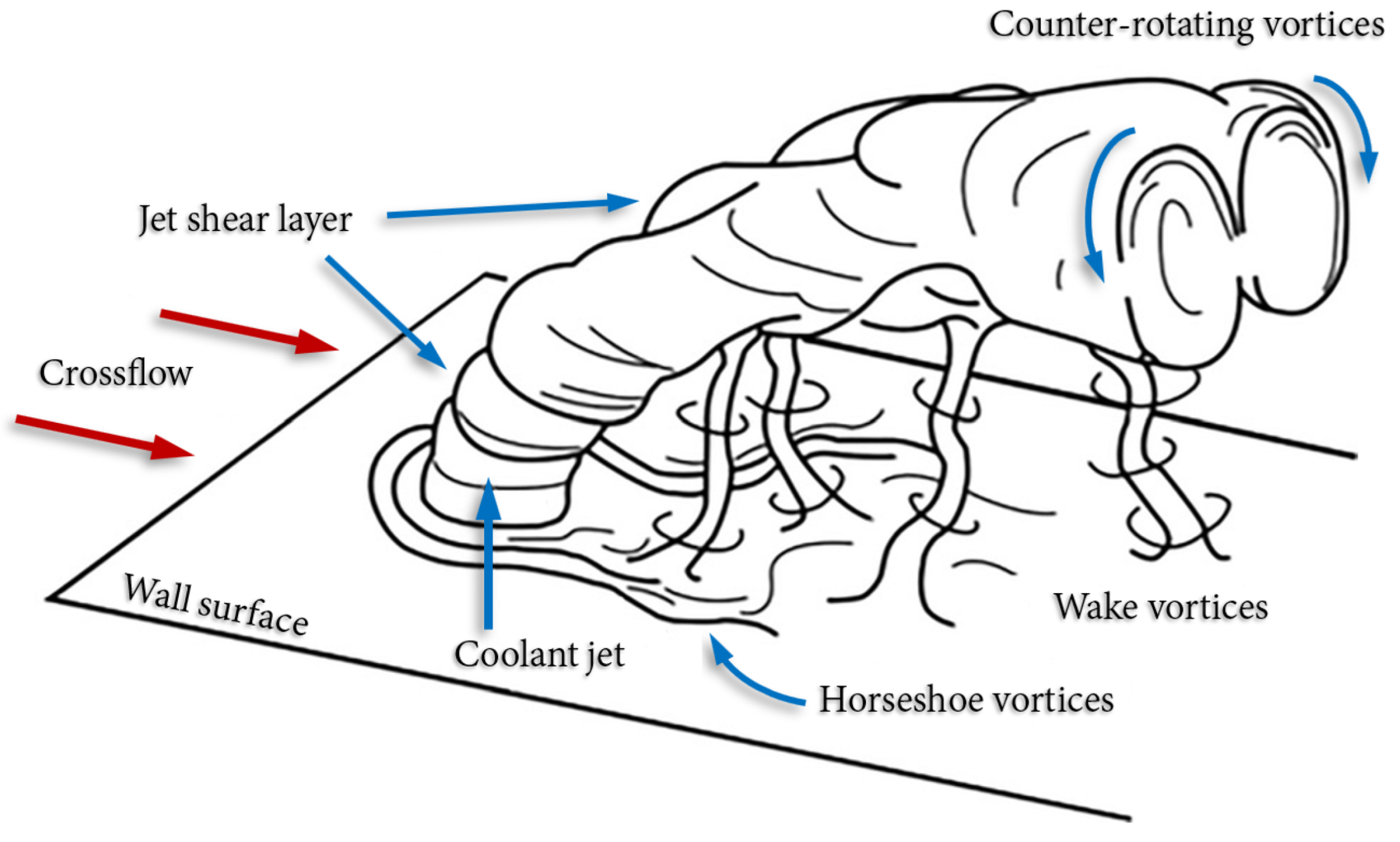
1. Introduction
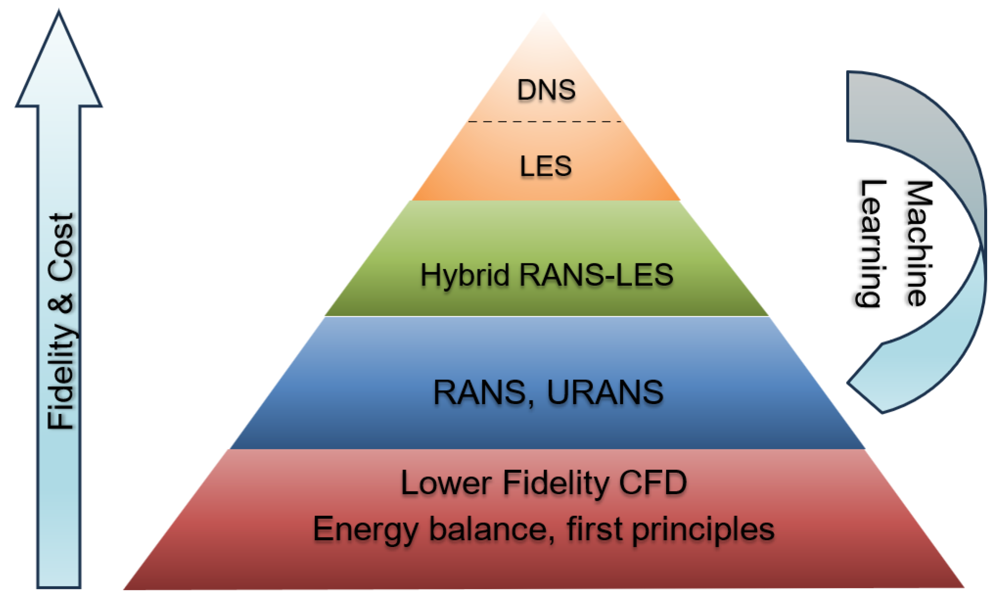
2. Overview of Numerical Methods and Challenges
3. Semi-Analytical Modelling
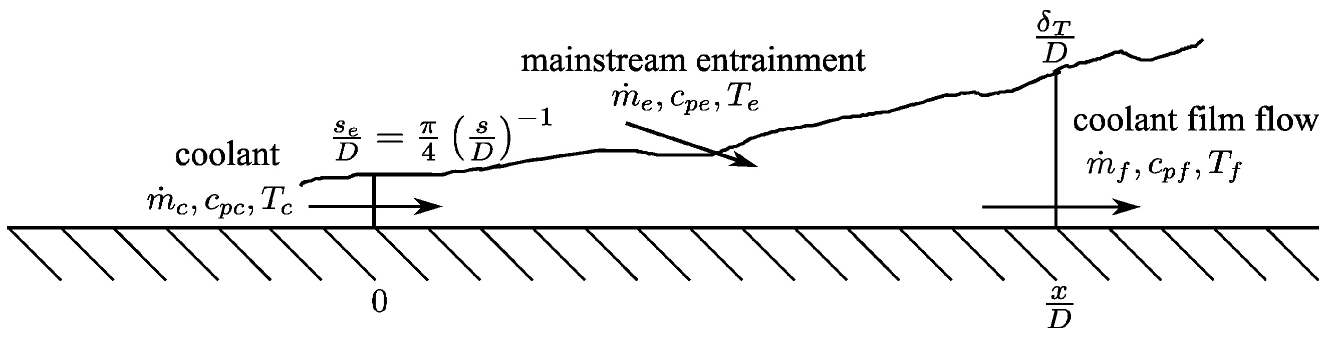
3.1. Single-Hole Models
3.2. Superposition Models
4. Reynolds-Averaged Navier–Stokes Modelling
4.1. Single Hole
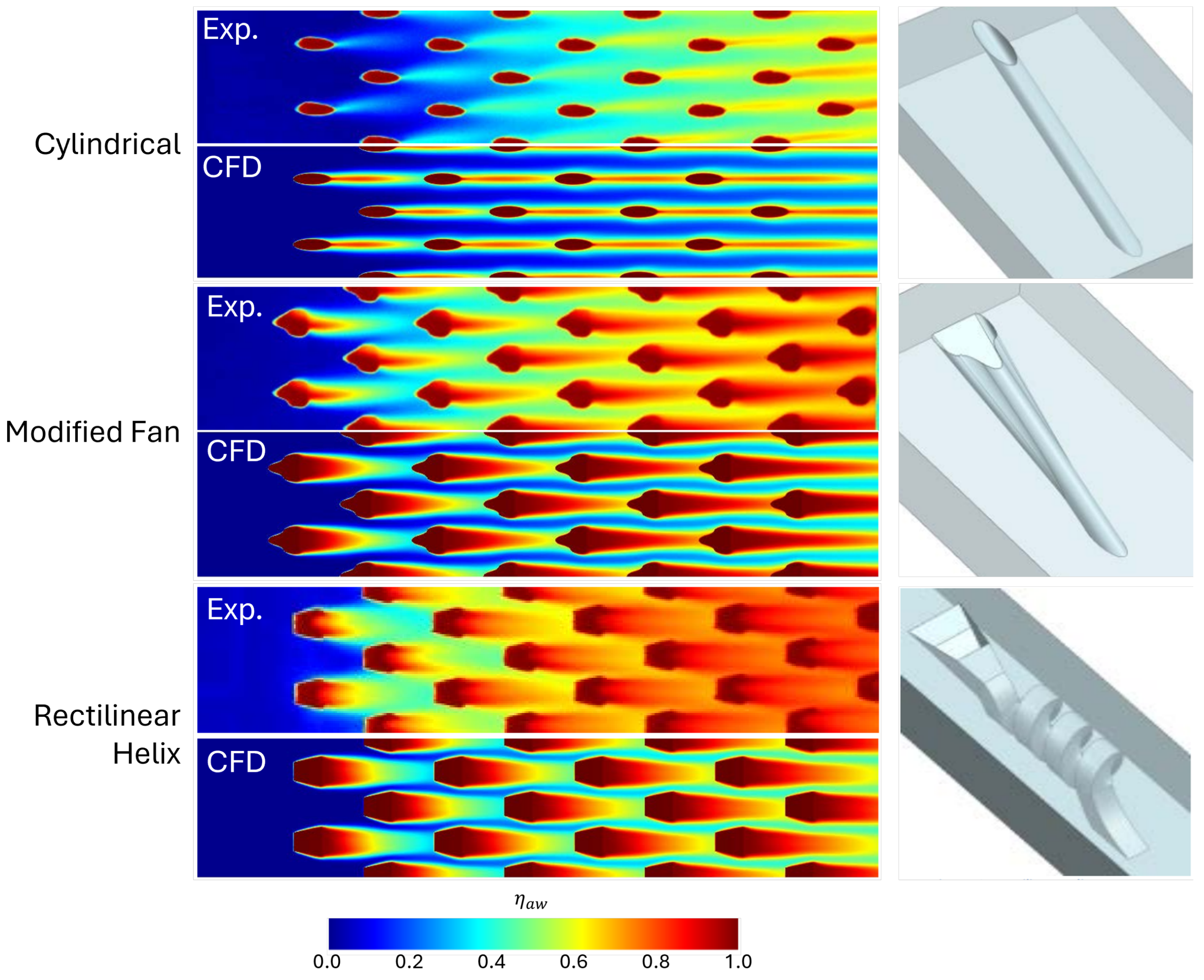
4.2. Multi-Hole
5. Hybrid RANS-LES
5.1. Single Hole
5.2. Multi-Hole
6. Large-Eddy Simulations
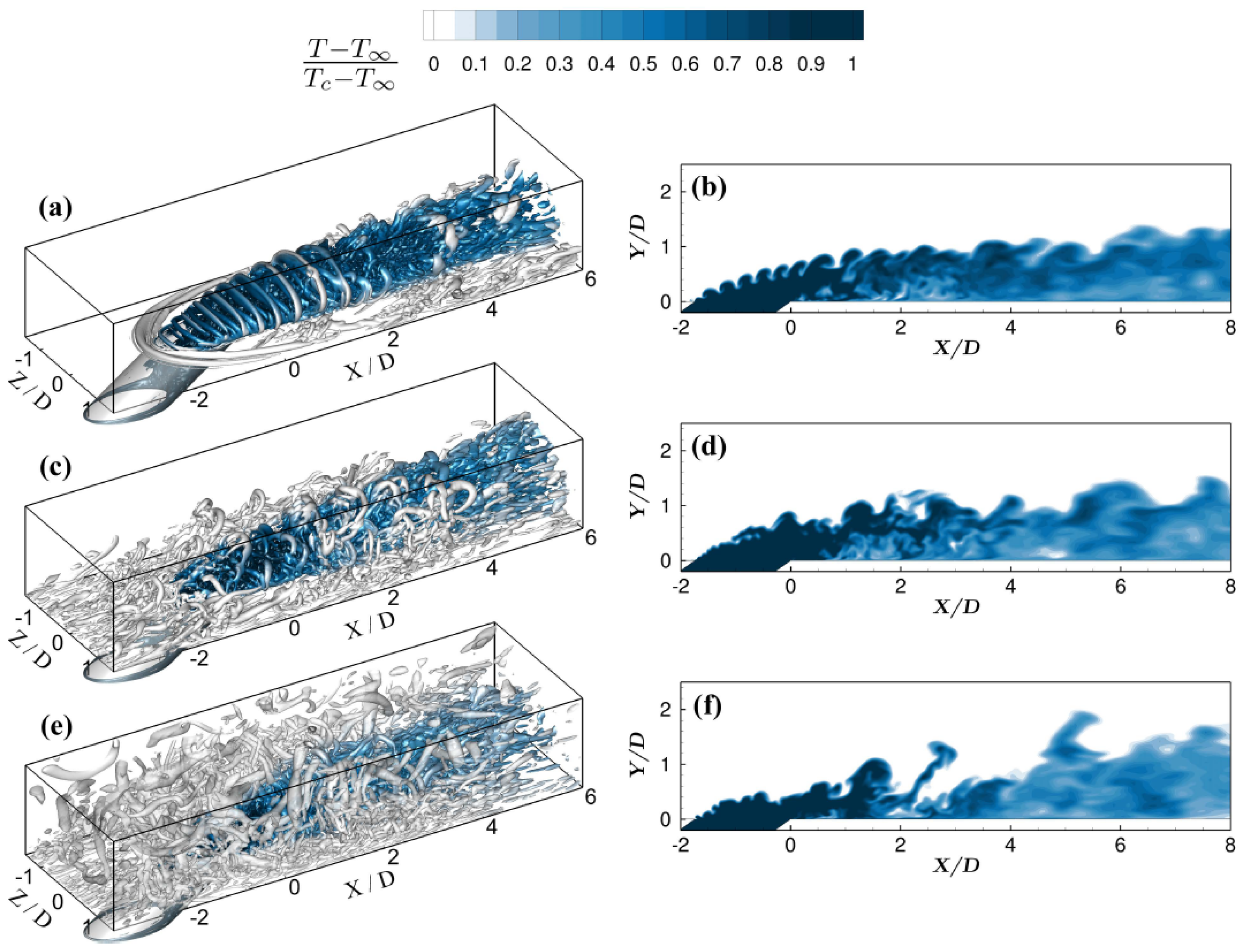
6.1. Single-Hole
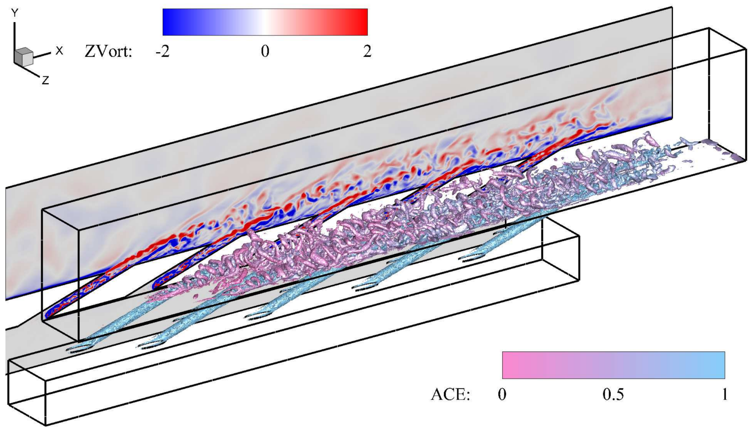
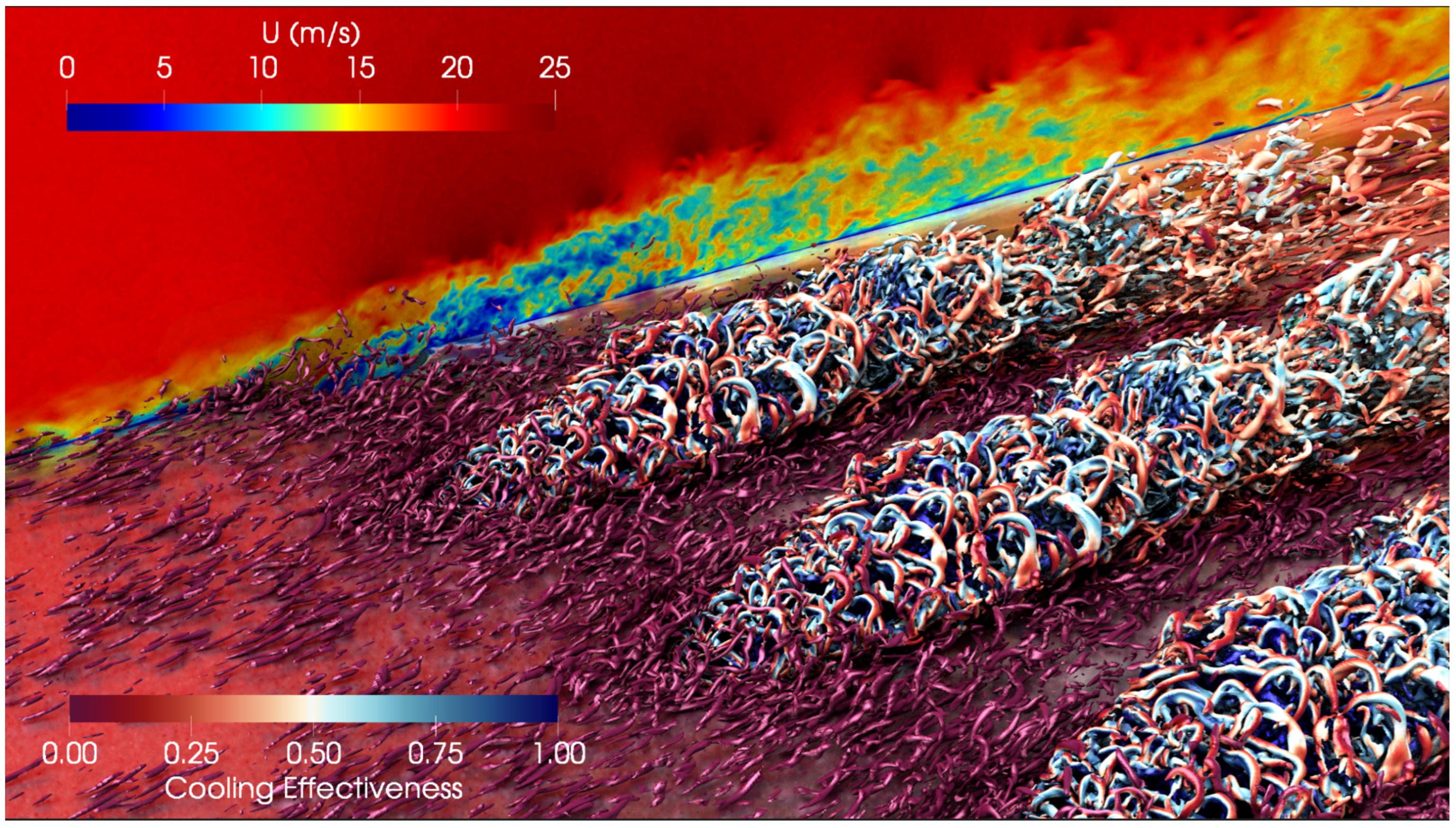
6.2. Multi-Hole
7. Machine Learning Augmented Modelling
8. Concluding Remarks and Outlook
- First-order principles and conservation law-based control volume methods are still relevant today. However, their practical usage is seen to have reduced, mainly due to the lower likelihood of canonical geometries and simplified boundary conditions.
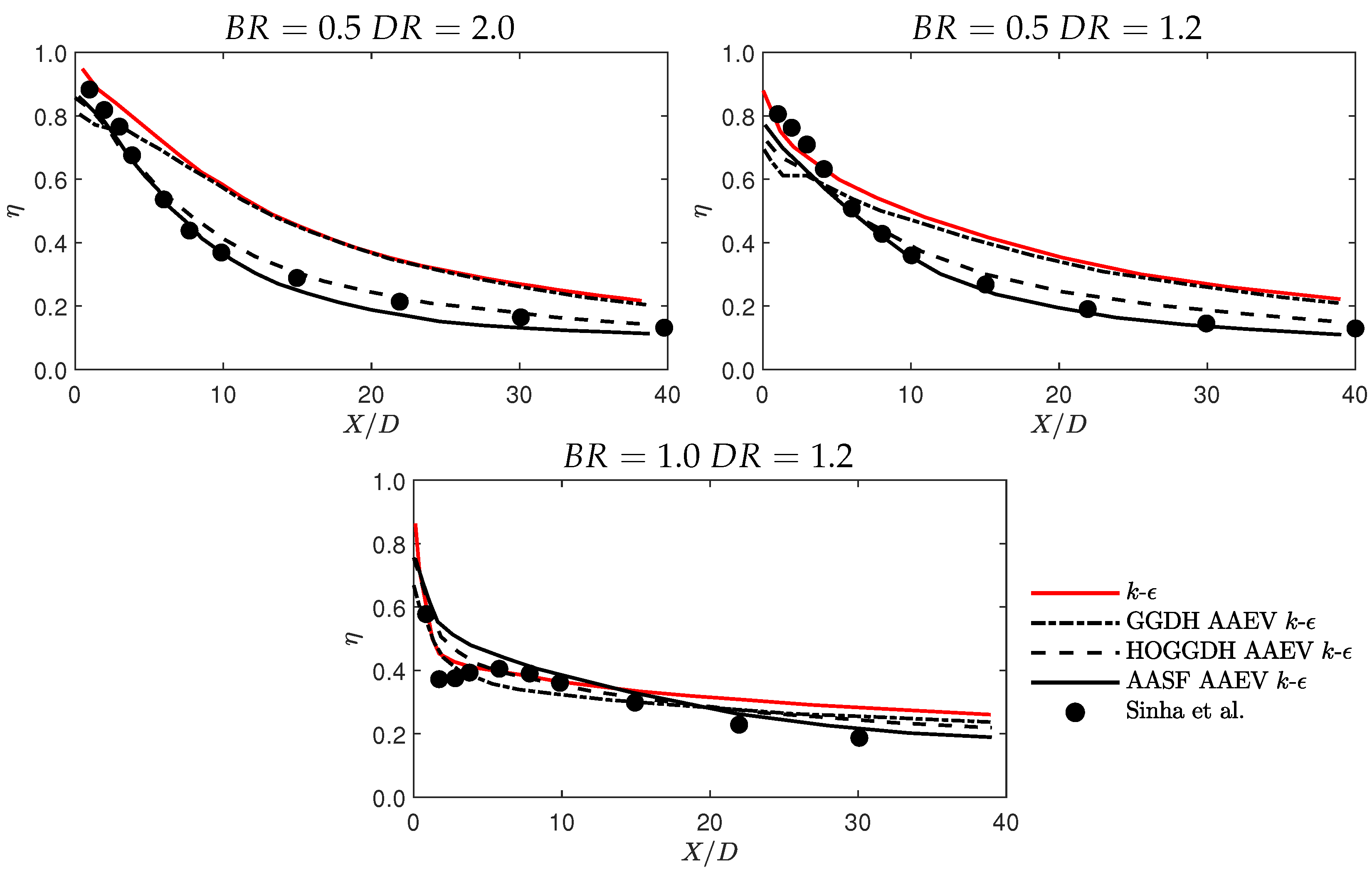
- For the RANS, however, there have been an overwhelming body of work producing reasonable results. RANS models tend to predict an elongation of coolant track in the streamwise direction while under-predicting the cooling jet’s lateral spreading. Mismatches of ACE distributions can be easily found in comparison studies against measurements, despite their superior computational efficiency to their higher-fidelity counterparts.
- Not surprisingly, eddy-resolving methods, which include LES and hybrid RANS-LES, have seen great increases in their application in practice, offering more accurate accounts for longitudinal and lateral distributions of ACE and surface temperature prediction. More importantly, they also come with the resolved Reynolds stresses and turbulent heat fluxes for interrogation that may reveal more underlying flow physics. However, these are at significant computational costs as our listed works have shown. In modern cooling designs, given the effectiveness strongly relies on the shape of the cooling holes, it would be impossible for eddy-resolving methods alone to provide all the answers to the vast varieties of design questions, leading to the next bullet point.
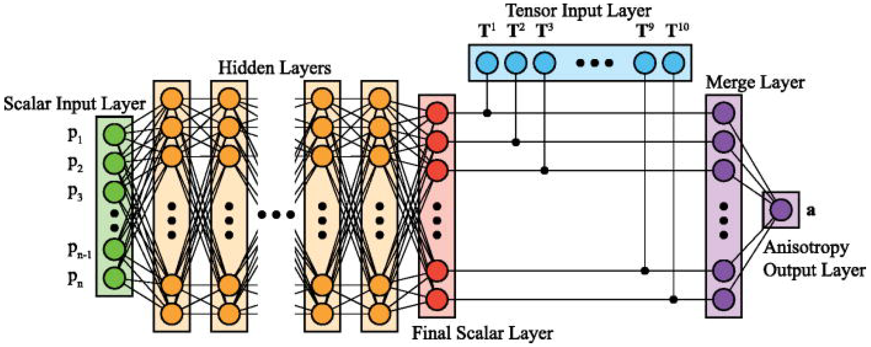
- The power of machine learning algorithms cannot be underestimated as they have demonstrated their huge potential to exploit the “big data” created by previously mentioned eddy-resolving methods. The physics-based input to the TBNN framework, for example, was shown to produce encouraging results.
Author Contributions
Funding
Data Availability Statement
Conflicts of Interest
Abbreviations
| ACE | Adiabatic cooling effectiveness |
| AHM | Adiabatic homogeneous model |
| AI | Artificial intelligence |
| ANN | Artificial neuron network |
| AVBP | Advanced virtual burner project |
| CFD | Computational fluid dynamics |
| CHT | Conjugate heat transfer |
| CNN | Convolution neural network |
| DDES | Delayed detached-eddy simulation |
| DES | Detached-eddy simulation |
| DMM | Dynamic mixed model |
| DNS | Direct numerical simulation |
| DRSM | Differential Reynolds stress model |
| GGDH | Generalized gradient diffusion hypothesis |
| HOGGDH | Higher-order generalised gradient diffusion hypothesis |
| LES | Large-eddy simulation |
| LHS | Latin hypercube sampling |
| MILES | Monotonically integrated LES |
| ML | Machine learning |
| MRC | Magnetic resonance concentration |
| PCA | Principal component analysis |
| RANS | Reynolds-averaged Navier–Stokes |
| SAFE | Source-based effusion model |
| SBES | Stress-blended eddy simulation |
| SGS | Sub-grid scale model |
| RNG | Re-Normalisation Group |
| RSM | Reynolds stress model |
| SAS | Scale Adaptive Simulation |
| SEM | Synthetic eddy method |
| SST | Shear stress transport model |
| TBNN | Tensor basis neural network |
| VLES | Very large eddy simulation |
| WALE | Wall-adaptive local eddy viscosity |
| GDH | Gradient diffusion hypothesis |
| ZDES | Zonal Detached-eddy simulation |
References
- Goldstein, R.J. Film cooling. Adv. Heat Transf. 1971, 7, 321–379. [Google Scholar]
- Wang, W.; Yan, Y.; Zhou, Y.; Cui, J. Review of Advanced Effusive Cooling for Gas Turbine Blades. Energies 2022, 15, 8568. [Google Scholar] [CrossRef]
- Aumeier, T.; Behrendt, T. Application of an Aerothermal Model for Effusion Cooling Systems and Finite Rate Chemistry in Aero-Engine Combustors. In Proceedings of the THMT15—8th International Symposium On Turbulence Heat and Mass Transfer, Sarajevo, Bosnia and Herzegovina, 15–18 September 2015. [Google Scholar] [CrossRef]
- Fric, T.F.; Roshko, A. Vortical structure in the wake of a transverse jet. J. Fluid Mech. 1994, 279, 1–47. [Google Scholar] [CrossRef]
- Chen, X. A Hybrid LES-RANS Approach for Effusion Cooling Prediction. Ph.D. Thesis, Loughborough University, Loughborough, UK, 2018. [Google Scholar]
- Chen, X.; Xia, H. Hybrid LES-RANS study of an effusion cooling array with circular holes. Int. J. Heat Fluid Flow 2019, 77, 171–185. [Google Scholar] [CrossRef]
- Chen, X.; Krawciw, J.; Xia, H.; Denman, P.; Bonham, C.; Carrotte, J. Study of an effusion-cooled plate with high level of upstream fluctuation. Appl. Therm. Eng. 2021, 184, 116126. [Google Scholar] [CrossRef]
- Ellis, C.D.; Xia, H.; Page, G.J. LES informed data-driven modelling of a spatially varying turbulent diffusivity coefficient in film cooling flows. In Turbo Expo: Power for Land, Sea, and Air, Proceedings of the ASME Turbo Expo 2020: Turbomachinery Technical Conference and Exposition, Virtual, 21–25 September 2020; American Society of Mechanical Engineers: New York, NY, USA, 2020; Volume 84171, p. V07BT12A029. [Google Scholar]
- Ellis, C.D.; Xia, H. Turbulent closure analysis in heated separated and reattached flow using eddy-resolving data. Phys. Fluids 2020, 32, 045115. [Google Scholar] [CrossRef]
- Ellis, C.; Xia, H. Impact of inflow turbulence on large-eddy simulation of film cooling flows. Int. J. Heat Mass Transf. 2022, 195, 123172. [Google Scholar] [CrossRef]
- Ellis, C.D.; Xia, H. Data-driven turbulence anisotropy in film and effusion cooling flows. Phys. Fluids 2023, 35, 105114. [Google Scholar] [CrossRef]
- Wilcox, D. Turbulence Modeling for CFD; Number v. 1 in Turbulence Modeling for CFD; DCW Industries: La Cañada, CA, USA, 2006. [Google Scholar]
- Choi, H.; Moin, P. Grid-point requirements for large eddy simulation: Chapman’s estimates revisited. Phys. Fluids 2012, 24, 011702. [Google Scholar] [CrossRef]
- Davidson, P. Turbulence: An Introduction for Scientists and Engineers; Oxford University Press: Oxford, UK, 2015. [Google Scholar]
- Spalart, P. Detached-Eddy Simulation. Annu. Rev. Fluid Mech. 2009, 41, 181–202. [Google Scholar] [CrossRef]
- Baldauf, S.; Schulz, A.; Wittig, S.; Scheurlen, M. An overall correlation of film cooling effectiveness from one row of holes. In Proceedings of the ASME 1997 International Gas Turbine and Aeroengine Congress and Exhibition, Orlando, FL, USA, 2–5 June 1997; American Society of Mechanical Engineers: New York, NY, USA, 1997; p. V003T09A010. [Google Scholar]
- Le Grives, E. Vorticity Associated with the Penetration of a Jet into a Cross Flow. J. Eng. Power JULY 1978, 100, 465. [Google Scholar] [CrossRef]
- Le Grives, E. Cooling Techniques for Modern Gas Turbines; Japikse, D., Ed.; Chapter 4 in Topics in Turbomachinery Technology; Concepts ETI, Inc.: Norwich, VT, USA, 1986. [Google Scholar]
- Keffer, J.F.; Baines, W.D. The round turbulent jet in a cross-wind. J. Fluid Mech. 1963, 15, 481–496. [Google Scholar] [CrossRef]
- Sinha, A.K.; Bogard, D.G.; Crawford, M.E. Film-cooling effectiveness downstream of a single row of holes with variable density ratio. J. Turbomach. 1991, 113, 442–449. [Google Scholar] [CrossRef]
- Sasaki, M.; Takahara, K.; Kumagai, T.; Hamano, M. Film Cooling Effectiveness for Injection from Multirow Holes. J. Eng. Power 1979, 101, 101–108. [Google Scholar] [CrossRef]
- Sellers, J.P. Gaseous film cooling with multiple injection stations. AIAA J. 1963, 1, 2154–2156. [Google Scholar] [CrossRef]
- Mayle, R.E.; Camarata, F.J. Multihole Cooling Film Effectiveness and Heat Transfer. J. Heat Transf. 1975, 97, 534–538. [Google Scholar] [CrossRef]
- Eckert, E.R.G. Analysis of Film Cooling and Full-Coverage Film Cooling of Gas Turbine Blades. J. Eng. Gas Turbines Power 1984, 106, 206–213. [Google Scholar] [CrossRef]
- Arcangeli, L.; Facchini, B.; Surace, M.; Tarchi, L. Correlative Analysis of Effusion Cooling Systems. J. Turbomach. 2008, 130, 011016. [Google Scholar] [CrossRef]
- Crawford, M.E.; Kays, W.M.; Moffat, R.J. Full-Coverage Film Cooling—Part I: Comparison of Heat Transfer Data for Three Injection Angles. J. Eng. Power 1980, 102, 1000–1005. [Google Scholar] [CrossRef]
- Crawford, M.E.; Kays, W.M.; Moffat, R.J. Full-Coverage Film Cooling—Part II: Heat Transfer Data and Numerical Simulation. J. Eng. Power 1980, 102, 1006–1012. [Google Scholar] [CrossRef]
- Andreini, A.; Facchini, B.; Picchi, A.; Tarchi, L.; Turrini, F. Experimental and Theoretical Investigation of Thermal Effectiveness in Multi-Perforated Plates for Combustor Liner Effusion Cooling. In Proceedings of the Turbo Expo: Power for Land, Sea, and Air, San Antonio, TX, USA, 3–7 June 2013; Volume 3C. Heat Transfer. [Google Scholar] [CrossRef]
- Andreini, A.; Da Soghe, R.; Facchini, B.; Mazzei, L.; Colantuoni, S.; Turrini, F. Local Source Based CFD Modeling of Effusion Cooling Holes: Validation and Application to an Actual Combustor Test Case. J. Eng. Gas Turbines Power 2014, 136, 011506. [Google Scholar] [CrossRef]
- Bergeles, G.; Gosman, A.D.; Launder, B.E.; Bergeles, G. The turbulent jet in a cross stream at low injection rates: A three-dimensional numerical treatment. Numer. Heat Transf. 1978, 1, 217–242. [Google Scholar] [CrossRef]
- Leylek, J.; Zerkle, R. Discrete-jet film cooling: A comparison of computational results with experiments. In Turbo Expo: Power for Land, Sea, and Air, Proceedings of the ASME 1993 International Gas Turbine and Aeroengine Congress and Exposition, Cincinnati, OH, USA, 24–27 May 1993; American Society of Mechanical Engineers: New York, NY, USA, 1993; Volume 78903, p. V03AT15A058. [Google Scholar]
- Walters, D.K.; Leylek, J.H. A Systematic Computational Methodology Applied to a Three Dimensional Film-Cooling Flowfield. In Proceedings of the ASME 1996 International Gas Turbine and Aeroengine Congress and Exhibition, Birmingham, UK, 10–13 June 1996. [Google Scholar]
- Walters, D.K.; Leylek, J.H. A detailed analysis of film-cooling physics Part 1: Streamwise injection with cylindrical holes. In Proceedings of the ASME 1997 International Gas Turbine and Aeroengine Congress and Exhibition, Orlando, FL, USA, 2–5 June 1997. [Google Scholar]
- Ferguson, J.D.; Walters, D.K.; Leylek, J.H. Performance of turbulence models and near-wall treatments in discrete jet film cooling simulations. In Turbo Expo: Power for Land, Sea, and Air, Proceedings of the ASME 1998 International Gas Turbine and Aeroengine Congress and Exhibition, Stockholm, Sweden, 2–5 June 1998; American Society of Mechanical Engineers: New York, NY, USA, 1998; Volume 78651, p. V004T09A077. [Google Scholar]
- Hoda, A.; Acharya, S. Predictions of a Film Coolant Jet in Crossflow With Different Turbulence Models. J. Turbomach. 2000, 122, 558–569. [Google Scholar] [CrossRef]
- Acharya, S.; Tyagi, M.; Hoda, A. Flow and heat transfer predictions for film cooling. Ann. N. Y. Acad. Sci. 2001, 934, 110–125. [Google Scholar] [CrossRef] [PubMed]
- Azzi, A.; Jubran, B.A. Numerical modeling of film cooling from short length stream-wise injection holes. Heat Mass Transf. 2003, 39, 345–353. [Google Scholar] [CrossRef]
- Harrison, K.L.; Bogard, D.G. Comparison of RANS turbulence models for prediction of film cooling performance. In Proceedings of the ASME Turbo Expo 2008: Power for Land, Sea, and Air, Berlin, Germany, 9–13 June 2008; Volume 43147, pp. 1187–1196. [Google Scholar]
- Li, X.; Ren, J.; Jiang, H. Application of algebraic anisotropic turbulence models to film cooling flows. Int. J. Heat Mass Transf. 2015, 91, 7–17. [Google Scholar] [CrossRef]
- Ling, J.; Ryan, K.J.; Bodart, J.; Eaton, J.K. Analysis of turbulent scalar flux models for a discrete hole film cooling flow. J. Turbomach. 2016, 138, 011006. [Google Scholar] [CrossRef]
- Laschet, G.; Rex, S.; Bohn, D.; Moritz, N. 3-D conjugate analysis of cooled coated plates and homogenization of their thermal properties. Numer. Heat Transf. Part A Appl. 2002, 42, 91–106. [Google Scholar] [CrossRef]
- Baldwin, B.; Lomax, H. Thin-layer approximation and algebraic model for separated turbulentflows. In Proceedings of the 16th Aerospace Sciences Meeting, Huntsville, AL, USA, 16–18 January 1978; p. 257. [Google Scholar]
- Bohn, D.; Krewinkel, R. Numerical investigation of the effectiveness of effusion cooling for plane multi-layer systems with different base-materials. Front. Energy Power Eng. China 2009, 3, 406–413. [Google Scholar] [CrossRef]
- Ceccherini, A.; Facchini, B.; Tarchi, L.; Toni, L. Adiabatic and overall effectiveness measurements of an effusion cooling array for turbine endwall application. In Proceedings of the ASME Turbo Expo 2008: Power for Land, Sea, and Air, Berlin, Germany, 9–13 June 2008. [Google Scholar]
- Ceccherini, A.; Facchini, B.; Tarchi, L.; Toni, L.; Coutandin, D. Combined effect of slot injection, effusion array and dilution hole on the heat transfer coefficient of a real combustor liner. In Proceedings of the ASME Turbo Expo 2009: Power for Land, Sea and Air, Orlando, FL, USA, 8–12 June 2009. [Google Scholar]
- Andreini, A.; Ceccherini, A.; Facchini, B.; Coutandin, D. Combined effect of slot injection, effusion array and dilution hole on the heat transfer coefficient of a real combustor liner part 2: Numerical analysis. In Proceedings of the ASME Turbo Expo 2010: Power for Land, Sea and Air, Glasgow, UK, 14–18 June 2010. [Google Scholar]
- Coletti, F.; Benson, M.J.; Ling, J.; Elkins, C.J.; Eaton, J.K. Turbulent transport in an inclined jet in crossflow. Int. J. Heat Fluid Flow 2013, 43, 149–160. [Google Scholar] [CrossRef]
- Andrei, L.; Andreini, A.; Bianchini, C.; Caciolli, G.; Facchini, B.; Mazzei, L.; Picchi, A.; Turrini, F. Effusion Cooling Plates for Combustor Liners: Experimental and Numerical Investigations on the Effect of Density Ratio. Energy Procedia 2014, 45, 1402–1411. [Google Scholar] [CrossRef]
- Ledezma, G.A.; Lachance, J.; Wang, G.; Wang, A.; Laskowski, G.M. Experimental and Numerical Investigation of Effusion Cooling for High Pressure Turbine Components: Part 2—Numerical Results. In Turbo Expo: Power for Land, Sea, and Air, Proceedings of the ASME Turbo Expo 2016: Turbomachinery Technical Conference and Exposition, Seoul, South Korea, 13–17 June 2016; American Society of Mechanical Engineers: New York, NY, USA, 2016; Volume 49798, p. V05BT17A002. [Google Scholar]
- Krawciw, J. Optimisation Techniques for Combustor Wall Cooling. Ph.D. Thesis, Loughborough University, Loughborough, UK, 2017. [Google Scholar]
- Launder, B.; Spalding, D. The numerical computation of turbulent flows. Comput. Methods Appl. Mech. Eng. 1974, 3, 269–289. [Google Scholar] [CrossRef]
- Pietrzyk, J.R.; Bogard, D.G.; Crawford, M.E. Effects of density ratio on the hydrodynamics of film cooling. J. Turbomach. 1990, 112, 437–443. [Google Scholar] [CrossRef]
- Pietrzyk, J.R.; Bogard, D.G.; Crawford, M.E. Hydrodynamic measurements of jets in crossflow for gas turbine film cooling applications. J. Turbomach. 1989, 111, 139–145. [Google Scholar] [CrossRef]
- Quarmby, A.; Quirk, R. Measurements of the radial and tangential eddy diffusivities of heat and mass in turbulent flow in a plain tube. Int. J. Heat Mass Transf. 1972, 15, 2309–2327. [Google Scholar] [CrossRef]
- Quarmby, A.; Quirk, R. Axisymmetric and non-axisymmetric turbulent diffusion in a plain circular tube at high Schmidt number. Int. J. Heat Mass Transf. 1974, 17, 143–147. [Google Scholar] [CrossRef]
- Bodart, J.; Coletti, F.; Bermejo-Moreno, I.; Eaton, J.K. High-fidelity simulation of a turbulent inclined jet in a crossflow. Cent. Turbul. Res. Annu. Res. Briefs 2013, 19, 263–275. [Google Scholar]
- Roy, S.; Kapadia, S.; Heidmann, J.D. Film Cooling Analysis Using DES Turbulence Model. In Proceedings of the Turbo Expo: Power for Land, Sea, and Air, Atlanta, GA, USA, 16–19 June 2003; Turbo Expo 2003, Parts A and B. Volume 6, pp. 1113–1122. [Google Scholar] [CrossRef]
- Foroutan, H.; Yavuzkurt, S. Numerical Simulations of the Near-Field Region of Film Cooling Jets Under High Free Stream Turbulence: Application of RANS and Hybrid URANS/Large Eddy Simulation Models. J. Heat Transf. 2015, 137, 011701. [Google Scholar] [CrossRef]
- Jin, Y.; Lu, L.; Huang, Z.; Han, X. Numerical investigation of flat-plate film cooling using Very-Large Eddy Simulation method. Int. J. Therm. Sci. 2022, 171, 107263. [Google Scholar] [CrossRef]
- Zamiri, A.; You, S.J.; Chung, J.T. Large eddy simulation of unsteady turbulent flow structures and film-cooling effectiveness in a laidback fan-shaped hole. Aerosp. Sci. Technol. 2020, 100, 105793. [Google Scholar] [CrossRef]
- Mazzei, L.; Andreini, A.; Facchini, B.; Turrini, F. Impact of Swirl Flow on Combustor Liner Heat Transfer and Cooling: A Numerical Investigation With Hybrid Reynolds-Averaged Navier–Stokes Large Eddy Simulation Models. J. Eng. Gas Turbines Power 2015, 138, 051504. [Google Scholar] [CrossRef]
- Mazzei, L.; Picchi, A.; Andreini, A.; Facchini, B.; Vitale, I. Unsteady Computational Fluid Dynamics Investigation of Effusion Cooling Process in a Lean Burn Aero-Engine Combustor. J. Eng. Gas Turbines Power 2016, 139, 011502. [Google Scholar] [CrossRef]
- Lenzi, T.; Palanti, L.; Picchi, A.; Bacci, T.; Mazzei, L.; Andreini, A.; Facchini, B. Time-Resolved Flow Field Analysis of Effusion Cooling System With Representative Swirling Main Flow. J. Turbomach. 2020, 142, 061008. [Google Scholar] [CrossRef]
- Arroyo-Callejo, G.; Laroche, E.; Millan, P.; Leglaye, F.; Chedevergne, F. Numerical Investigation of Compound Angle Effusion Cooling Using Differential Reynolds Stress Model and Zonal Detached Eddy Simulation Approaches. J. Turbomach. 2016, 138, 101001. [Google Scholar] [CrossRef]
- Zhang, C.; Lin, Y.; Xu, Q.; Liu, G.; Song, B. Cooling effectiveness of effusion walls with deflection hole angles measured by infrared imaging. Appl. Therm. Eng. 2009, 29, 966–972. [Google Scholar] [CrossRef]
- Tyagi, M.; Acharya, S. Large eddy simulation of film cooling flow from an inclined cylindrical jet. J. Turbomach. 2003, 125, 734–742. [Google Scholar] [CrossRef]
- Iourokina, I.; Lele, S. Towards large eddy simulation of film-cooling flows on a model turbine blade with free-stream turbulence. In Proceedings of the 43rd AIAA Aerospace Sciences Meeting and Exhibit, Reno, NV, USA, 10–13 January 2005; p. 670. [Google Scholar]
- Lund, T.S.; Wu, X.; Squires, K.D. Generation of turbulent inflow data for spatially-developing boundary layer simulations. J. Comput. Phys. 1998, 140, 233–258. [Google Scholar] [CrossRef]
- Renze, P.; Schroder, W.; Meinke, M. Large-eddy simulation of film cooling flows with variable density jets. Flow Turbul. Combust. 2008, 80, 119–132. [Google Scholar] [CrossRef]
- Renze, P.; Schroder, W.; Meinke, M. Large-eddy simulation of film cooling flows at density gradients. Int. J. Heat Fluid Flow 2008, 29, 18–34. [Google Scholar] [CrossRef]
- Guo, X.; Schröder, W.; Meinke, M. Large-eddy simulations of film cooling flows. Comput. Fluids 2006, 35, 587–606. [Google Scholar] [CrossRef]
- Rozati, A.; Tafti, D.K. Effect of coolant–mainstream blowing ratio on leading edge film cooling flow and heat transfer–LES investigation. Int. J. Heat Fluid Flow 2008, 29, 857–873. [Google Scholar] [CrossRef]
- Vreman, A.W. An eddy-viscosity subgrid-scale model for turbulent shear flow: Algebraic theory and applications. Phys. Fluids 2004, 16, 3670–3681. [Google Scholar] [CrossRef]
- Xie, Z.; Castro, I.P. Efficient generation of inflow conditions for large eddy simulation of street-scale flows. Flow. Turbul. Combust. 2008, 81, 449–470. [Google Scholar] [CrossRef]
- Oliver, T.A.; Bogard, D.G.; Moser, R.D. Large eddy simulation of compressible, shaped-hole film cooling. Int. J. Heat Mass Transf. 2019, 140, 498–517. [Google Scholar] [CrossRef]
- Immer, M.C. Time-Resolved Measurement and Simulation of Local Scale Turbulent Urban Flow. Ph.D. Thesis, ETH Zurich, Zurich, Switzerland, 2016. [Google Scholar]
- Kang, Y.S.; Rhee, D.H.; Song, Y.J.; Kwak, J.S. Large Eddy Simulations on film cooling flow behaviors with upstream turbulent boundary layer generated by circular cylinder. Energies 2021, 14, 7227. [Google Scholar] [CrossRef]
- Hao, M.; di Mare, L. Reynolds stresses and turbulent heat fluxes in fan-shaped and cylindrical film cooling holes. Int. J. Heat Mass Transf. 2023, 214, 124324. [Google Scholar] [CrossRef]
- Hao, M.; di Mare, L. Heat transfer and turbulent heat flux budgets in cooling films. Int. J. Heat Mass Transf. 2023, 217, 124687. [Google Scholar] [CrossRef]
- Hao, M.; di Mare, L. Budgets of Reynolds stresses in film cooling with fan-shaped and cylindrical holes. Phys. Fluids 2023, 35. [Google Scholar] [CrossRef]
- Hao, M.; Hope-Collins, J.; di Mare, L. Generation of turbulent inflow data from realistic approximations of the covariance tensor. Phys. Fluids 2022, 34, 115140. [Google Scholar] [CrossRef]
- Mendez, S.; Nicoud, F. Large-eddy simulation of a bi-periodic turbulent flow with effusion. J. Fluid Mech. 2008, 598, 27–65. [Google Scholar] [CrossRef]
- Renze, P.; Schro der, W.; Meinke, M. Large-eddy simulation of interacting film cooling jets. In Proceedings of the Turbo Expo: Power for Land, Sea, and Air, Orlando, FL, USA, 8–12 June 2009; Volume 48845, pp. 81–90. [Google Scholar]
- Motheau, E.; Lederlin, T.; Florenciano, J.L.; Bruel, P. LES investigation of the flow through an effusion-cooled aeronautical combustor model. Flow Turbul. Combust. 2012, 88, 169–189. [Google Scholar] [CrossRef]
- Smirnov, A.; Shi, S.; Celik, I. Random Flow Generation Technique for Large Eddy Simulations and Particle-Dynamics Modeling. J. Fluids Eng. 2001, 123, 359–371. [Google Scholar] [CrossRef]
- Konopka, M.; Jessen, W.; Meinke, M.; Schröder, W. Large-eddy simulation of film cooling in an adverse pressure gradient flow. J. Turbomach. 2013, 135, 031031. [Google Scholar] [CrossRef]
- El-Askary, W.; Schroeder, W.; Meinke, M. LES of compressible wall-bounded flows. In Proceedings of the 16th AIAA Computational Fluid Dynamics Conference, Orlando, FL, USA, 23–26 June 2003; p. 3554. [Google Scholar]
- Sung, Y.; Dord, A.L.; Laskowski, G.M.; Shunn, L.; Natsui, G.; Kapat, J. Detailed large eddy simulations (LES) of multi-hole effusion cooling flow for gas turbines. In Turbo Expo: Power for Land, Sea, and Air, Proceedings of the ASME Turbo Expo 2016: Turbomachinery Technical Conference and Exposition, Seoul, South Korea, 13–17 June 2016; American Society of Mechanical Engineers: New York, NY, USA, 2016; Volume 49798, p. V05BT17A017. [Google Scholar]
- Moin, P.; Squires, K.; Cabot, W.; Lee, S. A dynamic subgrid-scale model for compressible turbulence and scalar transport. Phys. Fluids A Fluid Dyn. 1991, 3, 2746–2757. [Google Scholar] [CrossRef]
- Vreman, B.; Geurts, B.; Kuerten, H. On the formulation of the dynamic mixed subgrid-scale model. Phys. Fluids 1994, 6, 4057–4059. [Google Scholar] [CrossRef]
- Lavrich, P.L.; Chiappetta, L.M. An Investigation of Jet in a Cross Flow for Turbine Film Cooling Applications; UTRC Report; United Technologies Research Center: East Hartford, CT, USA, 1990. [Google Scholar]
- Iourokina, I.; Lele, S. Large eddy simulation of film-cooling above the flat surface with a large plenum and short exit holes. In Proceedings of the 44th AIAA Aerospace Sciences Meeting and Exhibit, Reno, NV, USA, 9–12 January 2006; p. 1102. [Google Scholar]
- Iourokina, I.V.; Lele, S.K. Large eddy simulation of film cooling flow above a flat plate from inclined cylindrical holes. In Proceedings of the Fluids Engineering Division Summer Meeting, Miami, FL, USA, 17–20 July 2006; Volume 47500, pp. 817–825. [Google Scholar]
- Fureby, C.; Grinstein, F. Monotonically integrated large eddy simulation of free shear flows. AIAA J. 1999, 37, 544–556. [Google Scholar] [CrossRef]
- Jessen, W.; Schröder, W.; Klaas, M. Evolution of jets effusing from inclined holes into crossflow. Int. J. Heat Fluid Flow 2007, 28, 1312–1326. [Google Scholar] [CrossRef]
- Klein, M.; Sadiki, A.; Janicka, J. A digital filter based generation of inflow data for spatially developing direct numerical or large eddy simulations. J. Comput. Phy. 2003, 186, 652–665. [Google Scholar] [CrossRef]
- Wolf, P.; Staffelbach, G.; Roux, A.; Gicquel, L.; Poinsot, T.; Moureau, V. Massively parallel LES of azimuthal thermo-acoustic instabilities in annular gas turbines. Comptes Rendus Mec. 2009, 337, 385–394. [Google Scholar] [CrossRef]
- Hay, N.; Lampard, D.; Saluja, C. Effects of the condition of the approach boundary layer and of mainstream pressure gradients on the heat transfer coefficient on film-cooled surfaces. J. Eng. Gas Turbines Power. 1985, 107, 99–104. [Google Scholar] [CrossRef]
- Ham, F. An efficient scheme for large eddy simulation of low-Ma combustion in complex configurations. Annu. Res. Briefs Cent. Turbul. Res. Stanf. Univ. 2007, 41–45. [Google Scholar]
- Duraisamy, K.; Spalart, P.R.; Rumsey, C.L. Status, Emerging Ideas and Future Directions of Turbulence Modeling Research in Aeronautics; Technical Report NF1676L-28239, NASA Technical Reports Server: NTRS; U.S. National Aeronautics and Space Administration: Washington, DC, USA, 2017. [Google Scholar]
- Ling, J.; Ruiz, A.; Lacaze, G.; Oefelein, J. Uncertainty analysis and data-driven model advances for a jet-in-crossflow. J. Turbomach. 2017, 139, 021008. [Google Scholar] [CrossRef]
- Milani, P.M.; Ling, J.; Saez-Mischlich, G.; Bodart, J.; Eaton, J.K. A machine learning approach for determining the turbulent diffusivity in film cooling flows. J. Turbomach. 2017, 140, 021006. [Google Scholar] [CrossRef]
- Milani, P.M.; Ling, J.; Eaton, J.K. Physical interpretation of machine learning models applied to film cooling flows. J. Turbomach. 2019, 141, 011004. [Google Scholar] [CrossRef]
- Milani, P.M.; Ling, J.; Eaton, J.K. Generalization of machine-learned turbulent heat flux models applied to film cooling flows. J. Turbomach. 2020, 142, 011007. [Google Scholar] [CrossRef]
- Milani, P.M.; Ling, J.; Eaton, J.K. Turbulent scalar flux in inclined jets in crossflow: Counter gradient transport and deep learning modelling. arXiv 2020, arXiv:2001.04600. [Google Scholar] [CrossRef]
- Ellis, C.D.; Xia, H. LES Informed Data-driven Models for RANS Simulations of Single-hole Cooling Flows. Int. J. Heat Mass Trans. 2024. [Google Scholar]
- Milani, P.M.; Ling, J.; Eaton, J.K. On the generality of tensor basis neural networks for turbulent scalar flux modeling. Int. Commun. Heat Mass 2021, 128, 105626. [Google Scholar] [CrossRef]
- Wang, C.; Liu, Y.; Zhang, J. Prediction of thermo-mechanical performance for effusion cooling by machine learning method. Int. J. Heat Mass Transf. 2023, 207, 123969. [Google Scholar] [CrossRef]
- Yang, L.; Dai, W.; Rao, Y.; Chyu, M.K. A machine learning approach to quantify the film cooling superposition effect for effusion cooling structures. Int. J. Therm. Sci. 2021, 162, 106774. [Google Scholar] [CrossRef]
- Yu, H.; Lou, J.; Liu, H.; Chu, Z.; Wang, Q.; Yang, L.; Rao, Y. A transfer learning method to assimilate numerical data with experimental data for effusion cooling. Appl. Therm. Eng. 2023, 224, 120075. [Google Scholar] [CrossRef]
- Paccati, S.; Mazzei, L.; Andreini, A.; Facchini, B. Reduced-order models for effusion modeling in gas turbine combustors. J. Turbomach. 2022, 144, 081013. [Google Scholar] [CrossRef]
- Huang, W.; Zhang, X.; Zhou, W.; Liu, Y. Learning time-averaged turbulent flow field of jet in crossflow from limited observations using physics-informed neural networks. Phys. Fluids 2023, 35, 025131. [Google Scholar] [CrossRef]
- Huang, W.; Zhang, X.; Shao, H.; Chen, W.; He, Y.; Zhou, W.; Liu, Y. Swirling flow field reconstruction and cooling performance analysis based on experimental observations using physics-informed neural networks. J. Glob. Power Propuls. Soc. 2024, 8, 141–153. [Google Scholar] [CrossRef]


 ] and TBNN-SST-GDH [
 ]. (b) Experimental dataset [•], SST-HOG [
 ] and TBNN-SST-HOG [
 ].
] and TBNN-SST-GDH []. (b) Experimental dataset [•], SST-HOG [] and TBNN-SST-HOG [].
].
] and TBNN-SST-GDH []. (b) Experimental dataset [•], SST-HOG [] and TBNN-SST-HOG [].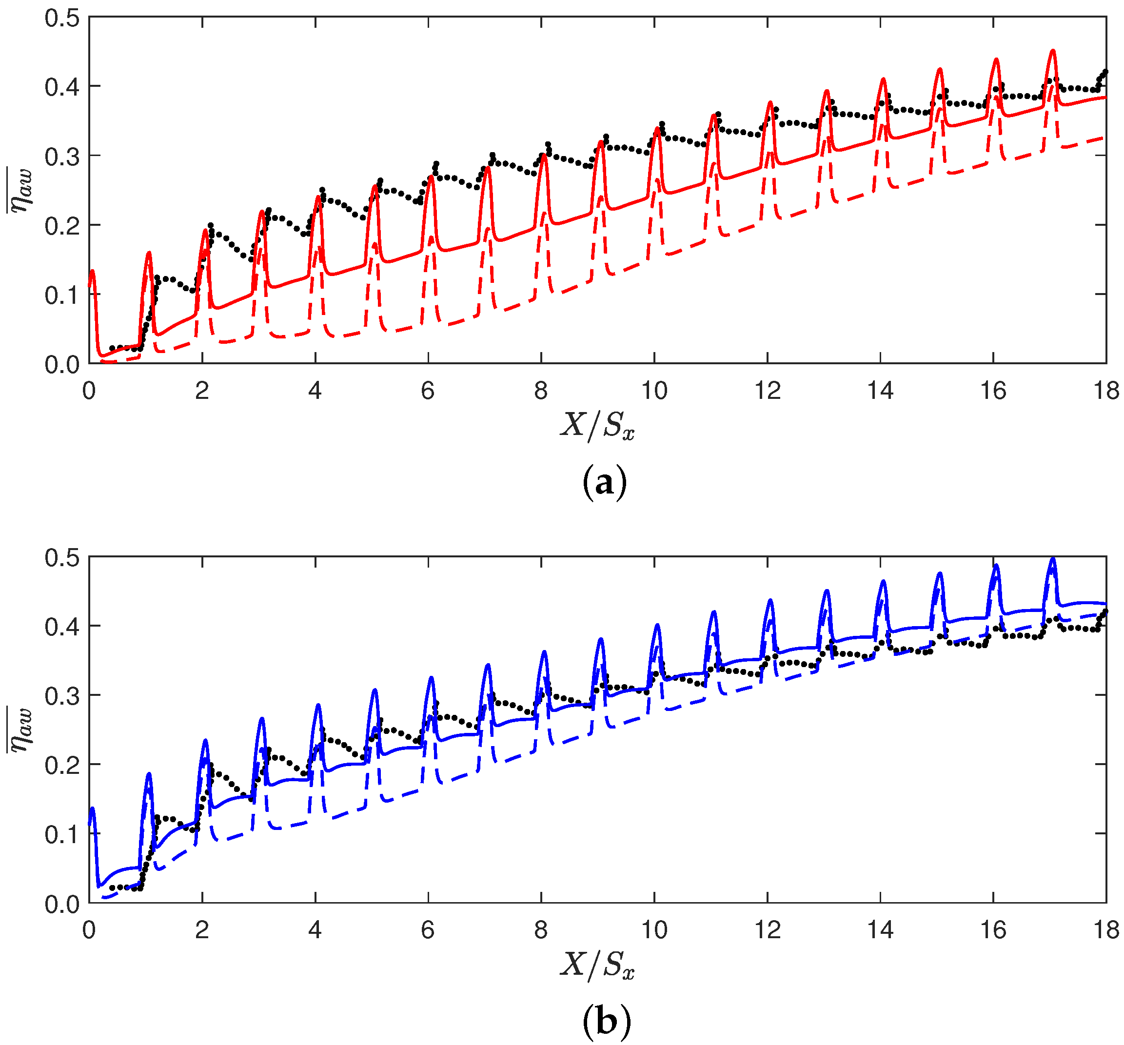

| Paper | Year | Turbulence Models | Turbulent Heat Flux |
|---|---|---|---|
| Bergeles et al. [30] | 1978 | Wall anisotropy model * | |
| Leylek and Zerkle [31] | 1993 | Standard k- | |
| Walters and Leylek [32] | 1996 | Launder–Spalding k- High Re | |
| Walters and Leylek [33] | 1996 | Launder–Spalding k- Two-layer | |
| Ferguson et al. [34] | 1998 | Standard k- two-layer wall model | |
| RNG k- | |||
| RSM * | |||
| Hoda and Acharya [35] | 2000 | High Re k- | |
| Low Re k- Launder–Sharma | |||
| Lam–Bremhost model | |||
| Low Re k- | |||
| DNS-based Low-Re k- | |||
| Low-Re Mayong–Kasagi * | |||
| Speziale * | |||
| Acharya et al. [36] | 2001 | k- | |
| RSM * | |||
| Azzi and Jubrain [37] | 2003 | k- with wall-based anisotropy model * | |
| Harrison and Bogard [38] | 2008 | Realizable k- | |
| Standard k- | |||
| RSM * | |||
| Li et al. [39] | 2015 | Algebraic anisotropic eddy viscosity model | Anisotropic scalar flux with GDH and HOGGDH |
| Ling et al. [40] | 2016 | Pseudo RANS with LES fields | GDH () |
| GDH ( from LES) | |||
| HOGGDH () | |||
| Laschet et al. [41] | 2002 | Algebraic eddy viscosity model [42] * | |
| Bohn and Krewinkel [43] | 2009 | Algebraic eddy viscosity model [42] * | |
| Ceccherini et al. [44] | 2008 | k- with wall-based anisotropy model [37] * | |
| Ceccherini et al. [45] | 2010 | SST Menter k- | |
| Andreini et al. [46] | 2010 | SST Menter k- | |
| Coletti et al. [47] | 2013 | Standard k- | GDH () |
| Andrei et al. [48] | 2014 | SST Menter k- with wall-based anisotropy model [37] * | |
| Ledezma [49] | 2016 | SST Menter k- with enhanced wall functions | |
| Realizable k- with enhanced wall functions | |||
| Krawciw [50] | 2017 | Two-layer realizable k- model | GDH |
| Case No. | Model | Parameter Value | Error |
|---|---|---|---|
| 1 | GDH | 0.013 | |
| 2 | GDH | 0.034 | |
| 3 | GDH | 0.023 | |
| 4 | HOGGDH | 0.031 | |
| 5 | HOGGDH | 0.020 |
| Paper | Year | Turbulence Models | Turbulent Inflow Model |
|---|---|---|---|
| Roy et al. [57] | 2009 | SA-DES | − |
| Foroutan and Yavuzkurt [58] | 2015 | realizable k--based DES | − |
| Chen and Xia [5] | 2018 | SST-based implicit LES | SEM |
| Jin et al. [59] | 2022 | k- based VLES | NA |
| LES-WALE | NA | ||
| SST-based DES | NA | ||
| Zamiri et al. [60] | 2020 | LES-WALE | NA |
| SST-based SAS | NA | ||
| DES | NA | ||
| Mazzei et al. [61] | 2015 | SST-based SAS | NA |
| SST-based DES | NA | ||
| Mazzei et al. [62] | 2016 | SST-based SAS | NA |
| Lenzi et al. [63] | 2020 | SST-based SBES | NA |
| Arroyo-Callejo et al. [64] | 2016 | DRSM | NA |
| SA-based Zonal DES | NA | ||
| k- SST | NA | ||
| Chen and Xia [5,6,7] | 2018–2021 | SST-based implicit LES | SEM |
| k- SST | NA |
| Paper | Year | Sub-Grid Scale Model | Turbulent Inflow Model |
|---|---|---|---|
| Tyagi and Acharya [66] | 2003 | DMM | No inflow turbulence |
| Iourokina and Lele [67] | 2005 | Dynamic Smagorinsky | Recycle-Rescaling [68] |
| Renze et al. [69,70] | 2008 | MILES | Recycle-Rescaling |
| Guo et al. [71] | 2006 | Implicit | Recycle-Rescaling [68] |
| Rozati and Tafti [72] | 2008 | Dynamic Smagorinsky () | No inflow turbulence |
| Bodart et al. [56] | 2013 | Vreman’s eddy viscosity model [73] | Digital filtering [74] |
| Oliver et al. [75] | 2019 | WALE | No inflow turbulence |
| Ellis and Xia [10] | 2022 | WALE () | Digital filtering [76] |
| Kang et al. [77] | 2021 | WALE | Turbulence generated by upstream cylinders |
| Hao and di Mare [78,79,80] | 2023 | Implicit | Digital filtering [81] |
| Mendez et al. [82] | 2008 | WALE | Periodic (assumes asymptotic effusion behaviour) |
| Renze et al. [83] | 2009 | MILES | No inflow turbulence |
| Motheau et al. [84] | 2012 | WALE | Synthetic turbulence [85] |
| Standard Smagorinsky | Synthetic turbulence [85] | ||
| Konopka et al. [86] | 2013 | Recycle-Rescaling [87] | |
| Sung et al. [88] | 2016 | Implicit wall resolved and modelled | No inflow turbulence |
| Ledezma [49] | 2016 | WALE | No inflow turbulence |
Disclaimer/Publisher’s Note: The statements, opinions and data contained in all publications are solely those of the individual author(s) and contributor(s) and not of MDPI and/or the editor(s). MDPI and/or the editor(s) disclaim responsibility for any injury to people or property resulting from any ideas, methods, instructions or products referred to in the content. |
© 2024 by the authors. Licensee MDPI, Basel, Switzerland. This article is an open access article distributed under the terms and conditions of the Creative Commons Attribution (CC BY) license (https://creativecommons.org/licenses/by/4.0/).
Share and Cite
Xia, H.; Chen, X.; Ellis, C.D. Modelling and Simulation of Effusion Cooling—A Review of Recent Progress. Energies 2024, 17, 4480. https://doi.org/10.3390/en17174480
Xia H, Chen X, Ellis CD. Modelling and Simulation of Effusion Cooling—A Review of Recent Progress. Energies. 2024; 17(17):4480. https://doi.org/10.3390/en17174480
Chicago/Turabian StyleXia, Hao, Xiaosheng Chen, and Christopher D. Ellis. 2024. "Modelling and Simulation of Effusion Cooling—A Review of Recent Progress" Energies 17, no. 17: 4480. https://doi.org/10.3390/en17174480
APA StyleXia, H., Chen, X., & Ellis, C. D. (2024). Modelling and Simulation of Effusion Cooling—A Review of Recent Progress. Energies, 17(17), 4480. https://doi.org/10.3390/en17174480