Optimising Flywheel Energy Storage Systems: The Critical Role of Taylor–Couette Flow in Reducing Windage Losses and Enhancing Heat Transfer

Abstract

Amidst the growing demand for efficient and sustainable energy storage solutions, Flywheel Energy Storage Systems (FESSs) have garnered attention for their potential to meet modern energy needs. This study uses Computational Fluid Dynamics (CFD) simulations to investigate and optimise the aerodynamic performance of FESSs. Key parameters such as radius ratio, aspect ratio, and rotational velocity were analysed to understand their impact on windage losses and heat transfer. This study reveals the critical role of Taylor–Couette flow on the aerodynamic performance of FESSs. The formation of Taylor vortices within the airgap was examined, demonstrating their effect on temperature distribution and overall system performance. Through a detailed examination of the skin friction coefficient and Nusselt number under different conditions, this study identified a nonlinear relationship between rotor temperature and rotational speed, highlighting the accelerated temperature rise at higher speeds. The findings indicate that optimising these parameters can significantly enhance the efficiency of FESSs, reducing windage losses and improving heat transfer. This research provides valuable insights into the aerodynamic and thermal optimisation of FESSs, offering pathways to improve their design and performance. The results contribute to advancing guidelines for the effective implementation of FESSs in the energy sector, promoting more sustainable energy storage solutions.

1. Introduction

Flywheel Energy Storage Systems (FESSs) are pivotal in the energy storage landscape due to their high energy density, rapid charging and discharging capabilities, long lifespan, and quick response for short-duration, high-cycle applications [1]. These systems are vital for effectively harnessing renewable energy sources such as solar and wind by mitigating supply and demand fluctuations, thus ensuring a continuous power supply [2]. Recent advancements, such as incorporating high-speed motors and magnetic levitation bearings into flywheels, have broadened their industrial applications, presenting significant opportunities for energy saving and emissions reduction [3]. Additionally, the deployment of flywheel energy storage arrays enhances grid stability by providing inertia support during sudden large power shortages, improving the grid’s frequency response, and addressing challenges related to active power support and frequency disturbance resistance [4].

The primary drawback of FESSs is the high mechanical losses, originating from bearing and aerodynamic “windage” losses [5]. Bearing losses, influenced by the flywheel mass and lubricant choice, increase linearly with flywheel speed. Windage losses, caused by friction between the rotor and the surrounding fluid, are particularly significant in high-speed applications and substantially contribute to increased self-discharge and thus lower overall FESS efficiency [6]. These losses result from the frictional interaction between the rotor and the working fluid, dissipating energy as heat, thus reducing system performance [1]. Gurumurthy et al. [7] found that mechanical losses, primarily due to drag, accounted for 72% of total losses in FESSs at high speeds.

Taylor [8] theoretically studied laminar flow between concentric cylinders and discovered an unstable flow structure characterised by complex toroidal vortices. This instability occurs when the angular velocity of the inner cylinder surpasses a certain value. In such scenarios, the centrifugal forces resulting from the rotation of a Couette flow dominate the viscous forces, leading to flow instability and the emergence of a secondary flow. These steady alternate vortices, known as ‘Taylor vortices’, occur under specific flow conditions [8]. Taylor vortex flow is characterised by the Taylor number, which facilitates the classification of potential flow regimes within the annulus of concentric cylinders. In the unstable regime, various complex spatial flow features such as spirals, modulated waves, and Taylor cells can be observed. The Taylor number enables the categorisation of potential flows in a system with an inner rotating cylinder and an outer stationary cylinder into several types: Couette flow (laminar flow), Taylor vortex flow (TVF), Wavy Vortex Flow (WVF), Modulated Wavy Vortices (MWV), turbulent Taylor vortices (TTV), and featureless turbulent flow (TUR) [9]. In FESSs, the flow within the airgap can exhibit three distinct patterns: Taylor–Couette flow, occurring where the cylinder face meets the housing; Von Karman flow, existing between the discs and housing [10], and an “Intermediate Region” at the intersection of the two aforementioned flows.

The stability of Taylor–Couette flow within the annulus of a FESS is essential for managing windage losses. This flow is extensively studied in fluid mechanics, particularly in high-speed electric motors where windage loss and heat transfer are critical factors [11]. Methods proposed by Nakane [12] and Pfister [13], such as using rotor shrouds or adjusting airgap size, have shown improvements in torque and power efficiency. Awad and Martin [14] explored windage losses on the disc and cylinder sides of pulse generator rotors, noting that the skin friction coefficient is influenced by the Taylor number, which is used to determine flow characteristics in concentric cylinders.

Heat transfer within FESSs, influenced significantly by Taylor–Couette flow, also impacts windage losses. Early research by Gazley [15] and subsequent studies by Becker and Kaye [15] and Tachibana et al. [16] have examined heat transfer in concentric cylinder annuli, emphasising the impact of airgap size on heat generation and dissipation. Howey et al. [17] further analysed how airgap size affects convective heat transfer in high-speed electric motors, calculating surface convective heat transfer coefficients for thermal modelling of radial-flux and axial-flux electrical machines. A study on high-speed electric motors highlighted the significance of understanding windage losses and optimising air cooling to improve motor efficiency [18]. A CFD study on high-speed electric motors showed that optimising axial air cooling can significantly reduce windage losses and meet temperature requirements, proposing a novel heat transfer correlation for such systems [19].

The objective of this study is to investigate the influence of Taylor–Couette flow on the performance of FESSs by examining the impact of airgap size and rotational velocity on windage losses. By focusing on these parameters, this study aims to understand how variations in the annular gap between the flywheel and the housing, as well as changes in rotational speed, affect the frictional losses and resulting energy dissipation. This research seeks to provide insights into optimising the design and operational conditions of FESS to minimise windage losses, thereby enhancing the overall efficiency and performance. The novelty of this study lies in its detailed exploration of the complex fluid dynamics within the airgap, particularly the role of Taylor–Couette flow, which has been underexplored in the existing literature. By providing a comprehensive analysis of how these flow dynamics influence thermal and aerodynamic characteristics, this research offers a new pathway for improving the design and efficiency of FESSs.

2. Numerical Modelling

2.1. Governing Equations and Assumptions

This study aims to develop a numerical model of a FESS with a smooth, narrow, and enclosed aigap design. Computational Fluid Dynamics (CFD) is employed to model the airflow structure within the annulus and predict the skin friction coefficient based on the velocity distribution. The CFD code utilises the governing equations based on the conservation laws [20]. The CFD domain for the enclosed FESS is created by dividing it into computational cells and nodes. The governing equations are then numerically discretised into a system of linear algebraic equations using the finite volume method, following the creation of the mesh [21]. The mass conservation equation, or continuity equation, is used to represent the rate of mass change within a fluid element [21].

2.2. Boundary Conditions and Mesh Generation

This section lays the groundwork for a comprehensive study of the factors influencing the aerodynamic performance of FESSs. This investigation is pivotal to selecting appropriate parameters for subsequent analysis aimed at optimising the aerodynamic efficiency of the FESS. Conceptually, a FESS is structured as a concentric cylinder comprising a rotating inner cylinder and a stationary outer cylinder. The numerical estimation of windage losses, crucial for this study, is derived from the computation of the rotor skin friction coefficient.

In this study, the airgap is defined using a dimensionless parameter known as the radius ratio (RR), denoted by $\eta =r_o/(r_o+g)$, where $r_o$ is the rotor radius and $g$ is the airgap width. Another critical parameter is the aspect ratio $\mathsf{\Gamma }=L/g$, where $L$ is the rotor length. The rotor radius and length have been set to 0.13 m. To align with the objective of the final FESS design being compact, the RR is constrained to maintain a narrow airgap.

Table 1. Studied FESS geometries.

Design	Gap $\mathit{g}$ (mm)	Radius Ratio $\mathit{\eta }$	Aspect Ratio $\mathbf{\Gamma }$
1	1.3	0.99	100
2	2.6	0.98	50
3	4.0	0.97	32.5
4	5.4	0.96	24
5	6.8	0.95	19

presents the values of the studied FESS geometries. The maximum rotational velocity of the rotor is set at 2400 rad/s, with peripheral speeds tested ranging from 6.5 to 312 m/s. Figure 1 depicts the FESS used in this investigation; due to the symmetrical nature of the FESS geometry, the CFD domain is reduced to an 8-degree segment with a central symmetry plane, significantly reducing the computational time and cost. Periodic boundary conditions are applied to the surfaces on either side of this 8-degree segment to accurately model the full computational domain.

Mesh independence analysis constitutes a critical pre-processing step in numerical simulations, serving to enhance the accuracy and reliability of the results. The number of elements used in this investigation and the dimensions of each mesh component are detailed in

Table 2. Mesh independence test parameters.

Mesh Number	Case	Element Number	Gap	Rotor and Housing
			Element Size (mm)
1	0.99	908,028	0.2	2
2		1,340,936	0.175	1.75
3		1,867,804	0.15	1.5
4		2,889,173	0.125	1.25
5		4,672,452	0.1	1
1	0.98	1,180,415	0.2	2
2		1,729,824	0.175	1.75
3		2,535,730	0.15	1.5
4		3,952,091	0.125	1.25
5		6,890,190	0.1	1
1	0.97	1,479,895	0.2	2
2		2,220,412	0.175	1.75
3		3,270,519	0.15	1.5
4		5,222,153	0.125	1.25
5		9,358,620	0.1	1
1	0.96	1,821,634	0.2	2
2		2,686,524	0.175	1.75
3		4,033,366	0.15	1.5
4		6,642,483	0.125	1.25
5		11,915,970	0.1	1
1	0.95	2,136,892	0.2	2
2		3,092,805	0.175	1.75
3		4,745,840	0.15	1.5
4		7,777,068	0.125	1.25
5		14,561,976	0.1	1

. All airgap models employed in this study utilise a structured quadrilateral mesh. The primary aim of this process is to identify a mesh configuration that yields solutions independent of the mesh size. This objective was pursued by conducting a mesh independence test, focusing on the rotor skin friction coefficient and the Nusselt number as key parameters of interest, at the highest rotational speed of 2400 rad/s.

The relationship between the skin friction coefficient and the Nusselt number, and the number of mesh elements for the five RRs studied, is depicted in Figure 2. Based on the outcomes of these tests, a mesh configuration comprising an airgap element size of 0.125 mm and a rotor and housing element size of 1.25 mm was selected. This configuration was chosen to optimise computational efficiency, as further increasing the mesh size showed negligible impact on the accuracy of the numerical results, indicating that the numerical predictions had become mesh-independent.

In this research, high mesh quality was maintained by closely monitoring mesh metrics. By maintaining the mesh orthogonal quality above 0.8, the mesh cells align closely with the computational domain’s coordinate directions, which is crucial for minimising numerical diffusion and improving the precision of gradient calculations. This level of orthogonality is particularly important when resolving complex flow patterns and thermal effects that are sensitive to mesh geometric fidelity.

2.3. Solver

The investigation of the steady-state operation of the simplified FESS was conducted using CFD. These simulations utilised steady-state models, with time-averaged steady-state solutions for the relative motion of the rotor using the moving reference frame technique. Due to the high peripheral Reynolds number of the rotor, calculated at $1.02\times {10}^{-6}$, the use of a turbulence model was necessitated. The RANS equations were solved using the SST k-omega turbulence model due to its effectiveness in handling complex flow conditions similar to those studied in this research [22]. The k–ω model, which forms the basis for the SST variant, can be referenced from the foundational work in turbulence modelling [23]. Additionally, references [19,24,25] were included to justify the model selection, as they describe similar flow conditions using the k–ω SST model.

The numerical analysis was streamlined by making several key assumptions: gravity was disregarded, the air was treated as an ideal gas, and the system was assumed to have no inlets or outlets. The thermal conditions of the housing were defined with a free stream temperature of 24 °C and a heat transfer coefficient of 30 W/m²·K, with all components initialised at this temperature. The computational model employed double precision for enhanced accuracy and utilised a pressure-based solver, integrating the energy equation into the solution process with a coupled solution method. It maintained second-order accuracy in pressure discretisation and the QUICK scheme for discretising various parameters. Wall treatment models were implemented to define flow profiles in the wall boundary layers, addressing the limitations of turbulence models in accounting for the viscous-affected region of the boundary layer. The wall cell ${\mathrm{y}}_{+}\le 1$ was used to create a boundary layer mesh with a high resolution in order to resolve the viscous sublayer.

2.4. Validation

Figure 3 compares the predicted average velocity profile with experimental data from prior investigations by Hosain et al. [26] and H. Reichardt [27]. For a balanced comparison, the simulated velocity values were normalised to match the range of the experimental data. The non-dimensional coordinates $X=-1$ and $X=1$ correspond to the housing and rotor walls, respectively. At low Reynolds numbers, the velocity profile shows a linear inclination, while at higher Reynolds numbers, a pronounced gradient near the walls is evident due to wall-bound viscous forces. The midpoint of the airgap represents the point of average velocity. The computed average velocity profile closely matches the empirically observed profiles, with similar trends reported in earlier studies [28,29]. Empirical findings from the authors further validate the CFD model [30]. The experimental FESS was connected to an electric motor via a transmission system, enabling rotation up to 40,000 RPM. The flywheel comprises an inner steel hub and an outer reinforced carbon fibre ring. The geometrical dimensions are as follows: the flywheel case diameter is 320 mm, the flywheel diameter is 260 mm, the flywheel width is 130 mm, and the airgap size is 1.33 mm. The maximum tested rotational speed in this investigation was 14,000 RPM. Both experimental and numerical results show comparable flow characteristics, with deviations between the two data sets confined within a maximum 15% margin of error.

2.5. Flow Characterisation

Windage losses can be calculated by analysing the flow within the airgap. The power required from the system to overcome the windage losses of a rotating cylinder can be calculated using Equation (1) [31]:

$$P_w=\left(M_D+M_c\right)\omega$$

(1)

where $\omega$ is the rotational velocity of the rotor, $M_D$ is the disc moment on the side, and $M_c$ is the rotor moment, which can be calculated using Equations (2) and (3), respectively.

$$M_D={\rho \omega }^2{r_o}^5{C}_m$$

(2)

$$M_c={\pi \rho \omega }^2{r_o}^{4}L{C}_w$$

(3)

where $\rho$ is the fluid density, $L$ is the rotor length, $r_o$ is the rotor radius, $C_m$ is the disc torque coefficient, and $C_w$ is the rotor skin friction coefficient. The Reynolds number of the working fluid within the airgap can be calculated using the following equation:

$${Re}_w={\displaystyle \frac{{\rho \omega r}_o\left(2g\right)}{\mu }}$$

(4)

where $(2g$) is the hydraulic diameter of the annulus and $g$ is the airgap size. The RR between the rotor and the housing is determined by the following relationship:

$$\eta ={\displaystyle \frac{r_o}{r_o+g}}$$

(5)

The classical inviscid criterion of rotational stability shows that Couette flow is unstable with an internal rotating cylinder and an outer cylinder at rest. If the clearance of the cylinder gap is relatively small compared to the cylinder radius, the flow depends on the Taylor number [32]:

$$T_a={\displaystyle \frac{\omega \times r_o\times g}{\upsilon }}{\left({\displaystyle \frac{g}{r_o}}\right)}^{0.5}$$

(6)

where $\upsilon$ is the kinematic viscosity. The Taylor number can be used to determine the flow characteristics as shown in Equation (7):

$$If\left\{\begin{array}{c}{T}_a<41.3 Laminar Couettw flow \\ 41.3<T_a<400 Laminar flow with cellular Taylor vortices\\ T_a>400 Turbulent flow \end{array}\right.$$

(7)

The Nusselt number for the Taylor flow can be calculated through various correlations. Becker and Kaye [33] developed a correlation to calculate the Nusselt number based on the Taylor number, as shown in Equation (8):

$$Nu=\left\{\begin{array}{c}2 T{a}_m<1700\\ {{0.128Ta}_m}^{0.367} 1700<T{a}_m<{10}^4\\ {{0.409Ta}_m}^{0.241} {10}^4<T{a}_m<{10}^7\end{array}\right.$$

(8)

where $T{a}_m$ is the modified Taylor number, which can be determined by Equation (9):

$$T{a}_m={\displaystyle \frac{Ta}{F_g}}$$

(9)

where $F_g$ is the geometrical factor expressed by Equation (10):

$$F_g={\displaystyle \frac{{\pi }^4\left[\frac{2r_o-2.304g}{2r_o-g}\right]}{1697\left[0.0056+0.0571{\left(\frac{2r_o-2.304g}{2r_o-g}\right)}^2\right]{\left[1-\frac{g}{2r_o}\right]}^2}}$$

(10)

If the airgap size is minimal compared to the rotor radius, then $F_g$ is close to unity, thus $T{a}_m$ is equal to $Ta$. Therefore, Gazley’s correlation [15] given by case Equation (11) can be used to calculate the Nusselt number:

$$Nu=\left\{\begin{array}{c}1.1 Ta<41\\ 0.117T{a}^{0.63}P{r}^{0.27} 41<Ta<100\\ 0.212T{a}^{0.5}P{r}^{0.27} 100<Ta<\infty \end{array}\right.$$

(11)

This comprehensive approach to characterising flow within the airgap of FESSs will provide critical insights into optimising the system to reduce windage losses and enhance overall system performance.

3. Results and Discussion

3.1. Flow Fields of the FESS

This study analyses the influence of Taylor–Couette flow on the air velocity distribution within the airgap of FESSs at different rotational speeds (200, 800, 1600, and 2400 rad/s) and radius ratios (RRs). As the rotational speed increases, the formation of Taylor vortices becomes more pronounced, leading to complex flow patterns. These vortices are more compact and frequent at higher speeds, significantly impacting heat transfer and windage losses. Figure 4 illustrates the air velocity distribution within the radial airgap with a RR of 0.99. The formation of Taylor–Couette flow within the annulus is responsible for the observed spike-shaped flow pattern. It is noted that air velocity near the housing approaches zero, while it reaches its peak near the rotor.

A critical Taylor number, indicative of flow instability, is reached at a rotational speed of 38 rad/s. Consequently, Taylor vortices form within the radial airgap at all the rotational speeds examined in this study. These vortices increase in intensity at higher rotational speeds. The velocity vector plot showcasing the Taylor vortices at various studied rotational speeds is presented in Figure 5, which exhibits symmetry along the axial direction. As the rotational speed increases, viscous forces are outweighed by inertial forces, leading to the formation of these vortices.

The size and compactness of Taylor vortices are influenced by the rotor speed. At higher speeds, the vortices appear more stretched, as illustrated in Figure 6. This effect results from the fact that vortices traverse less distance within a shorter time at higher speeds. This study demonstrates that Taylor vortex cells become progressively more compact as the rotational speed increases, a phenomenon primarily attributed to the reduced spatial travel of the vortices in a given timeframe.

The variation in airgap size has a significant impact on the number of Taylor vortices formed, as the wavelength of these vortices is approximately equal to twice the size of the airgap. The critical wavelength of the Taylor vortices can be estimated using the following equation [34]:

$${\lambda }_{cr}={\displaystyle \frac{2\pi g}{k_{cr}}}\approx 2g$$

(12)

where $k_{cr}$ represents the non-dimensional axial wave number at the onset of instability, which has a value of 3.12, and $g$ is the airgap size. This relationship suggests that the height of a Taylor cell is nearly equal to the gap size, resulting in a nearly square cell. However, it is important to note that this equation provides an approximation of the Taylor vortices’ wavelength and, while it offers a good representation of the number of Taylor vortices, it is not precise.

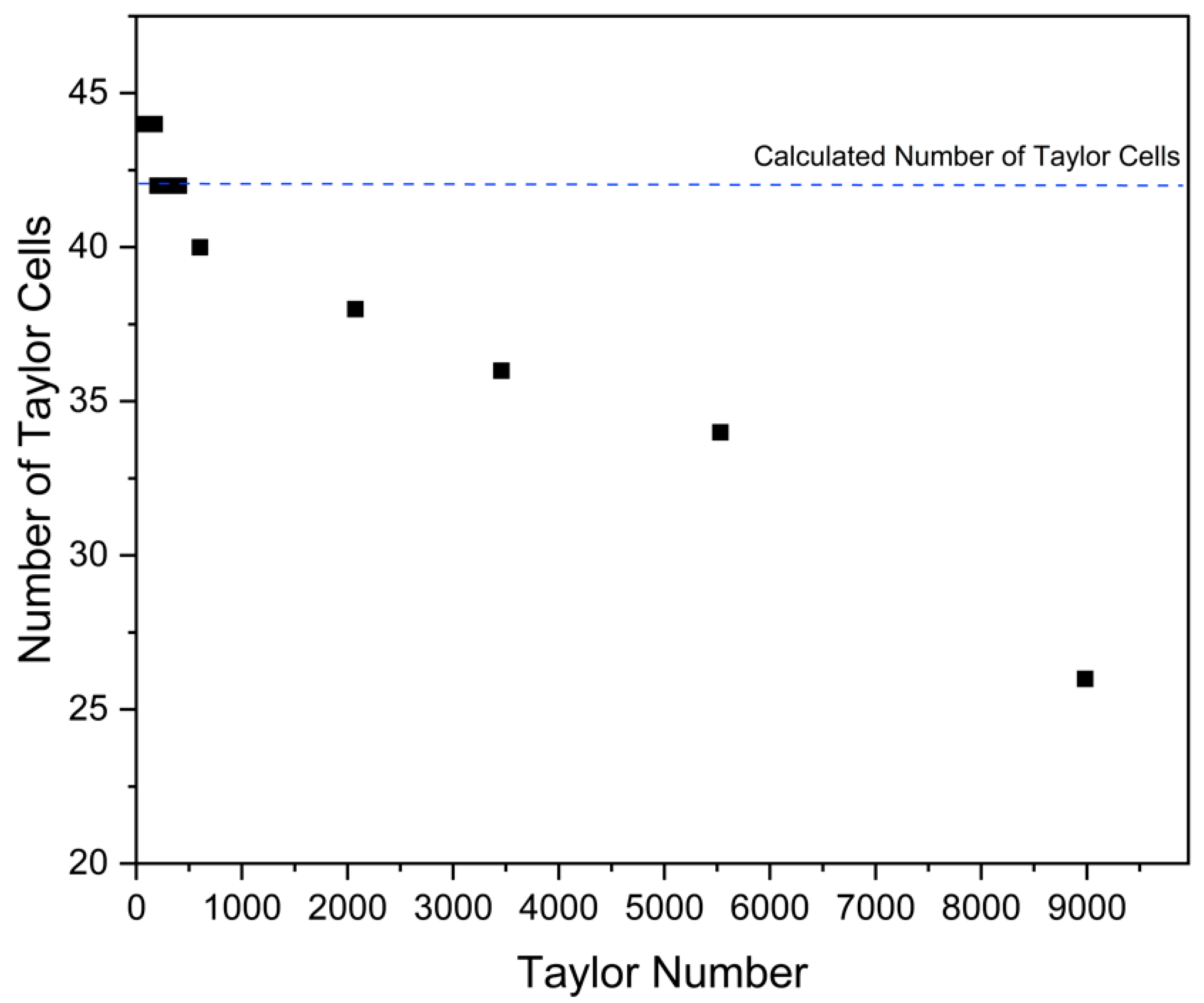
As the Taylor number increases, the discrepancy between the actual number of Taylor cells and the number calculated from this equation grows, as depicted in Figure 7. This is due to the fact that the equation primarily considers the system in terms of airgap size, whereas, in reality, a higher Taylor number leads to an intensified formation of Taylor vortices. This increase in vortex formation consequently affects the number of Taylor cells, making the Taylor vortices more dominant.

On the other hand, an increase in the radial airgap size results in a reduction in the number of Taylor vortices, as demonstrated in Figure 8. This phenomenon becomes evident when maintaining a constant rotational speed; in this case, as the airgap size increases, the number of Taylor vortices decreases. Further analysis reveals that the rotational velocity remains relatively consistent across various airgap sizes. This consistency is illustrated in Figure 9, which shows that despite changes in the radial airgap size, the rotational velocity remains almost uniform.

This study reveals a direct correlation between the number of Taylor vortices and the temperature within the FESS, specifically the rotor, housing, and the working fluid (i.e., air). This relationship is illustrated in Figure 10, where a decrease in the number of Taylor vortices corresponds to a reduction in the temperature across these components. Notably, the highest temperature within the system was recorded in the smallest airgap studied, while the lowest temperature in the housing was observed in the largest airgap size. The flow instability within the system manifests as counter-rotating toroidal vortices. This phenomenon is not only evident in the velocity contour plots but is similarly reflected in the temperature contour plots, underscoring the significant impact of Taylor vortices on air temperature distribution within the annulus. Consequently, it is observed that an increase in the number of Taylor vortices leads to a rise in the air temperature within the airgap.

Due to the rotation of the inner cylinder, the fluid particles located near the rotor encounter an increased centrifugal force, causing them to exhibit a propensity to move outward. The vortices cause the fluid with significant tangential momentum near the rotor to move outward in a radial direction, specifically in the regions where the flow is moving away between two neighbouring pairs of vortices. In a symmetrical manner, fluid with low velocity is transported from the vicinity of the stationary housing towards the centre in the regions where two neighbouring vortices meet, as shown in Figure 11. This process redistributes the rotational momentum of the fluid throughout the ring-shaped region. The subsequent redistribution of mass flow throughout the annulus impacts the velocity distribution of both the inward and outward flows. Therefore, the outward flow between the vortices is significantly more powerful than the inward flow.

An observed characteristic of the velocity vectors is the blending and transfer of momentum at the intersection of two neighbouring vortices. At this point, there is a substantial fluid mixture between neighbouring vortices. Each vortex contributes to the central mixing region of a vortex pair, located near the inner cylinder, and subsequently receives fluid from this mixing region, near the outer cylinder. A similar blending process takes place at the entrance area, where adjacent vortex pairs interact. Another notable observation regarding the velocity vectors is the movement of the vortex centres towards the outer cylinder. This phenomenon can be attributed to the flow regime being investigated at a high Reynolds number. At a high Reynolds number, the centrifugal force resulting from the rotation of the rotor exceeds the pressure gradient caused by the stationary housing wall. The disparity between these two forces results in the displacement of the vortex centre towards the outer cylinder wall.

Figure 12 presents a contour plot depicting the axial velocity in the Z-Y plane of the FESS for a RR of 0.96 at a rotational velocity of 1600 rad/s. This figure specifically highlights the radial airgap between the rotor and the housing, which is the primary area of interest in this study. The objective is to examine the influence of radial airgap size on the system performance. To facilitate a clearer understanding of the effects, especially in scenarios where the airgap is relatively small, a more focused section of the airgap has been selected for detailed analysis. Approximately one-third of the airgap width will be used for this purpose. This strategic selection enables a more visible and precise observation of the velocity changes across different airgap sizes.

Figure 13 illustrates the development of a recurring pattern of maximum and minimum axial velocities within the annulus at the four examined RRs. The observed flow pattern is a consequence of the rotor operating at high speed, resulting in a transition from a stable Couette flow to a Taylor vortex flow. This transition is characterised by the formation of vortices that extend across the radial airgap. The velocity maxima and minima are caused by the rotational movement of the vortex and are positioned in a radial direction above and below each vortex core, as shown in Figure 12. The zero contour lines in Figure 13 represent the radial positions of the central core of the vortices shown in Figure 12, which occur between the highest and lowest values. Figure 14 illustrates that each Taylor vortex rotating in a clockwise direction causes maximum axial velocity below its central core near the rotor wall and minimum axial velocity above its core near the housing wall on the Z-Y plane.

The contour plots in Figure 14 depict the radial velocity of the studied RRs at a rotational velocity of 1600 rad/s. These plots reveal a recurring pattern of alternating minimum and maximum values of radial velocity along the axial direction. The radial flow occurs as a result of the difference between the centrifugal forces applied to the fluid caused by the rotation of the rotor and the radial pressure gradients that restore equilibrium in the radial momentum of the flow. The amplitude of the alternating radial velocity maxima and minima is depicted at the centre of the corresponding concentric contours in Figure 14.

The contour plot utilises a colour scheme where the red lines represent positive values of radial velocity, while the blue lines represent negative values of radial velocity. The contour displays the rotational direction of the Taylor vortices through positive and negative values. A red contour cluster followed by a blue contour cluster in the positive axial direction indicates the presence of an anti-clockwise vortex on the Z-Y plane. In the same manner, the presence of a blue contour cluster followed by a red contour cluster indicates the occurrence of a Taylor vortex rotating in a clockwise direction. The contour clusters in Figure 14 display negative and positive values, which correspond to regions of inward flow and outward flow, respectively, which occur at the meeting point of adjacent vortices.

The highest values of radial velocity are observed in the regions of outward flow along the radial direction, as depicted in Figure 14, specifically at the location indicated in Figure 12. The points of lowest radial velocity can be observed in the regions where the flow is directed inward. One specific location of interest is indicated in Figure 12. The zero velocity contours correspond to the central positions of the vortices depicted in Figure 14. The observed flow pattern, characterised by alternating axial and radial velocity maxima and minima, in Figure 13 and Figure 14, is consistent and qualitatively agrees with previous CFD research and experimental measurements conducted by Deshmukh et al. [35], Deng et al. [36], and Adebayo [37].

Figure 15 displays the contour plots of the tangential velocity for the investigated RRs at a rotational velocity of 1600 rad/s. The contour plots display a minimum tangential velocity adjacent to the rotor wall and a maximum tangential velocity adjacent to the housing wall. The magnitude of the minimum tangential velocity exceeds that of the maximum tangential velocity. Specifically, the tangential velocity is highest in the vicinity of the rotor, aligning with the rotational direction of the rotor. This outcome is anticipated due to the convective fluid motion caused by the rotation of the rotor, which aligns with the solid body and reaches its highest angular velocity at the surface of the rotor. The negative tangential velocity is a result of the direction of rotation of the rotor, as indicated by the reference system in Figure 1.

The tangential velocity of the fluid possesses two characteristics: magnitude, which refers to the absolute value of the rotational speed, and direction. In this case, the rotor maintains a constant speed at its surface, and the direction of rotation of the rotor is specified as clockwise. The alteration in the orientation of the tangential velocity vectors within the azimuthal plane results in a centripetal force that is aimed towards the centre of the rotor. The red and blue colour codes on the contour plots represent the minimum and maximum negative values of tangential velocity, respectively.

In Figure 15, the contours exhibit outward bulging in the regions where fluid flows radially outward. This is due to the transport of high tangential momentum fluid by the Taylor vortices from the vicinity of the rotor towards the stationary housing. The contours exhibit radial inward bulging in the regions where the flow is directed inward, as the Taylor vortices transport low-momentum fluid from the stationary housing wall towards the rotor. The contour lines exhibit more pronounced curvature in the regions where the flow moves away from the centre compared to the regions where the flow moves towards the centre. This is because the Taylor vortex centres are closer to the outward flow saddle planes, leading to a higher radial velocity in the outward flow regions caused by the Taylor vortices. This feature also demonstrates the magnitude of the induced velocity caused by the Taylor vortices in these regions.

The air velocity distribution within the radial airgap, characterised by distinct RRs of 0.98, 0.97, and 0.96, respectively, follows a similar pattern to that of RR 0.99 (see Figure 4). A common observation across these RRs is the spike-shaped flow pattern, a characteristic feature of the Taylor–Couette flow. Adjacent to the housing, the air velocity is notably minimal, nearing zero, while it reaches its peak near the rotor. This pattern is consistent across the studied RRs. Additionally, an interesting phenomenon was observed, wherein an increase in the airgap size resulted in a reduction in the number of Taylor vortices. The reduction is quantitatively significant, as evidenced by the decrease in the number of vortices: from 22 vortices for a RR of 0.98 to 14 for a RR of 0.97, and down to 12 for a RR of 0.96. This trend underscores the influence of radial airgap size on the formation and number of Taylor vortices within the FESS annulus.

The size of the airgap plays a pivotal role in determining the number of Taylor vortices. Each Taylor cell consists of a pair of Taylor vortices, which typically exhibit a quadrilateral shape. Consequently, an increase in the airgap size leads to larger Taylor vortices, resulting in the formation of fewer Taylor cells. Within the FESS annulus, Taylor vortices exhibit a consistent symmetrical formation along the axial direction. This symmetry arises from the interplay of forces within the system. As the rotational velocity increases, inertial forces begin to outweigh viscous forces, leading to the formation of Taylor vortices. This phenomenon is particularly pronounced at higher speeds. A notable characteristic of Taylor vortices is the variation in their size and compactness, which are influenced by the rotor speed. At higher rotational speeds, these vortices tend to stretch more, similar to Figure 5 with a RR of 0.99.

Figure 16, Figure 17 and Figure 18 show the linear velocity within the airgap of the FESS at four rotational speeds: 200, 800, 1600, and 2400 rad/s. The data were collected from the centre of the airgap on the Y-Z plane. The rapid changes in the linear velocity are due to the Taylor vortices that form within the annulus. The wavelength of the Taylor vortices is equal to the distance between two adjacent spikes in Figure 16, Figure 17 and Figure 18. As the rotational velocity increases, so does the wavelength of the Taylor vortices. This is because the fluid has more inertia at higher rotational speeds, which allows the vortices to grow larger. The figures also show that the linear velocity distribution within the airgap is not symmetrical around the centre. This is because the Taylor vortices are not symmetrical. The vortices are typically stronger at the outer edge of the airgap than the inner edge since the working fluid has more inertia at the outer edge.

This study compares the theoretical and simulated wavelengths of Taylor vortices (Taylor cells) across various RRs. For a RR of 0.99, the theoretical wavelength derived from Equation (12) is 2.6 mm, suggesting the presence of 100 Taylor cells. However, the simulation results yield a slightly larger wavelength of 2.8 mm, resulting in a lower cell count of 92. As the airgap size increases, a notable reduction in the number of Taylor cells is observed. For instance, with a RR of 0.98, the theoretical calculation predicts 50 cells, whereas the simulation shows only 44 cells, each with a wavelength of 5.9 mm. This trend of fewer Taylor cells with larger airgap sizes is consistent for RRs of 0.97 and 0.96. Specifically, the simulation results for a 0.97 RR show a wavelength of 8.1 mm with 32 cells, and for a 0.96 ratio, the wavelength extends to 10.8 mm, corresponding to only 24 cells. This reduction in cell count with larger airgaps could be attributed to the limited space available for the formation of new Taylor cells. Importantly, the increase in the airgap size and the corresponding decrease in the number of Taylor cells contribute to enhanced heat transfer between the rotor, housing, and the working fluid. This improved heat transfer efficiency results in lower temperatures for each of the above-mentioned components, showcasing a critical aspect of thermal management in FESSs.

3.2. Characterisation of Windage Losses and Heat Transfer

This study analyses the effect of rotational speed on the rotor skin friction coefficient at five different RRs. The investigation reveals that the air velocity distribution within the airgap undergoes significant changes at different rotational speeds across all RRs, as shown in Figure 19. This change is attributed to the Taylor number surpassing the critical value of 41.3, leading to the formation of Taylor vortices.

As Figure 20 illustrates, the Taylor number increases as the rotational velocity, hence the Reynolds number increases, thereby complicating the flow dynamics. A notable observation is the dramatic drop in the skin friction coefficient value beyond a Taylor number of 1700. Beyond this point, changes in the coefficient with respect to the Taylor number become minimal. This phenomenon is linked to the boundary layers becoming thinner and more dispersed, indicative of a transition to turbulent flow.

Figure 21 presents the variation of the rotor skin friction coefficient as a function of rotational speed for different RRs. For all the studied RRs, the skin friction coefficient decreases sharply with an increase in rotational speed up to a certain point, after which the decrease levels off. This trend suggests that as the flywheel spins faster, the relative impact of skin friction on its performance diminishes, possibly due to the onset of turbulent flow, which reduces the relative effect of surface roughness. The curves suggest that the skin friction coefficient is also dependent on the RR, with higher RR values starting off with higher skin friction coefficients at lower speeds. This could be due to the increased surface area in contact with the fluid at higher RR values, leading to greater initial resistance. Additionally, the skin friction coefficient is influenced by the fluid density, which is in turn affected by the temperature of the system components. Figure 22 illustrates the correlation between the rotor temperature in Kelvin (K) and the rotational speed in radians per second (rad/s) for various RRs. There is a clear trend across all the studied RRs demonstrating that as the rotational speed increases, so does the rotor temperature. This positive correlation suggests that higher speeds lead to greater frictional forces, thus generating more heat. At lower speeds, the increase in temperature is relatively moderate; however, the curve becomes steeper beyond a certain value for all RRs. This steeper rise indicates a nonlinear relationship, where temperature rise accelerates at higher speeds, due to the exponential increase in frictional heating. This increase in temperature has a significant impact on the rotor skin friction coefficient.

Air friction is more significant in larger airgaps, this is due to the increasing rotor shear stress being exacerbated by the Taylor vortices. In fact, the critical Taylor number is reached in larger airgaps before the onset of these vortices in narrower airgaps, since the Taylor number is a function of the airgap size. The highest windage losses are produced by the smallest airgap. Figure 23 shows the windage losses in Watts (W) as a function of rotational speed for various RRs. There is a pronounced increase in windage losses as the rotational speed increases for all RRs due to greater air resistance. At lower speeds, the windage losses for different RRs appear very similar, but as speed increases, slight divergences emerge. This indicates that the flywheel geometry affects windage losses, but its impact becomes more noticeable at higher speeds. Initially, the increase in windage losses is gradual, but beyond a certain speed threshold, the losses rise more sharply. This nonlinear increase is attributed to the transition from laminar to turbulent flow, resulting in higher resistance thus greater windage losses.

Figure 24 illustrates the Reynolds number as a function of rotational speed for FESSs at various RRs. A Reynolds number is a dimensionless quantity used in fluid mechanics to predict flow regimes. For all RRs, as the rotational speed increases, so does the Reynolds number, indicating a shift towards more turbulent flow conditions. This is a known fluid flow characteristic around rotating objects, where increased speed leads to increased turbulence. Each curve peaks at a certain rotational speed, suggesting an optimal speed at which the flow transitions from laminar to turbulent for each RR value. Beyond this speed, the Reynolds number decreases, which is due to the change in flow characteristics as the temperature of the working fluid within the airgap rises with the increase in the rotational speed. This is mainly attributed to the change in the kinematic viscosity of the air as the temperature changes which leads to the creation of a reverse parabolic shape. The peak Reynolds number and the speed at which it occurs vary with the RR. Higher RRs reach higher Reynolds numbers, implying that a larger airgap experiences more significant turbulent flow effects at a given speed.

Figure 25 shows the Taylor number against the Reynolds number across the studied RRs. The graph shows a direct relationship between these two critical dimensionless parameters, indicating how the rotational effects are captured by the Taylor number and the inertial and viscous forces are represented by the Reynolds number. There is a direct and almost linear correlation between the Taylor number and the Reynolds number for each RR, as the inertial forces become more significant relative to viscous forces (higher Reynolds number), the impact of rotation on the flow (Taylor number) also increases. The graph displays different lines for each RR, indicating that the geometry of the flywheel affects how rotational effects scale with changes in the flow regime. Higher RRs show a steeper slope, which indicates that a larger airgap amplifies the rotational effects more significantly at the same increase in inertial forces.

Figure 26 presents the windage losses against the Taylor number for different RRs. The windage losses for all studied RRs initially increase with the Taylor number, indicating that as the flow becomes more influenced by rotational effects, the losses due to air resistance inside the FESS housing increase. Each RR displays a distinct relationship between the Taylor number and windage losses, suggesting that the flywheel airgap size significantly impacts the aerodynamic performance of the system. Higher RRs appear to be associated with higher windage losses at lower Taylor numbers. The curves demonstrate that the windage losses increase to a peak before declining sharply. The peak represents a critical point where the fluid flow likely transitions from stable to unstable, marked by the formation of turbulent Taylor vortices.

Figure 27 presents the relationship between the Nusselt number and the rotational speed for the studied RRs. The Nusselt number is a dimensionless parameter that describes the convective heat transfer relative to conductive heat transfer across a boundary. For all the studied RRs, the Nusselt number initially increases with the rotational speed, indicating enhanced convective heat transfer as the flywheel spins faster. This is because higher speeds increase fluid motion, thereby improving the heat transfer from the flywheel surface. Each curve peaks at a certain speed, which represents the point of maximum convective heat transfer efficiency for a given RR, beyond which the Nusselt number decreases. The graph shows that the peak Nusselt number and the speed at which it occurs vary with RR. Higher RRs reach higher Nusselt numbers at lower speeds, which is due to the Taylor number value and the number of Taylor vortices. The trend indicates that there is an optimal speed range for thermal management in FESSs, where convective cooling is most effective. Operating beyond this range could lead to less efficient cooling, which must be considered when designing the system.

The Nusselt number also varies with the Taylor number for different RRs, as shown in Figure 28. The trend shows that as the Taylor number increases, indicating more pronounced rotational effects, the Nusselt number also increases, suggesting that stronger rotational flow provides better mixing between cold and hot surfaces. On the other hand, higher RRs tend to have higher Nusselt numbers, indicating that the flywheel airgap can significantly influence the convective heat transfer characteristics of the system. Unlike previous figures where the Nusselt number peaks at certain speeds, here it shows steady growth with the Taylor number.

4. Conclusions

This study has comprehensively examined the influence of Taylor–Couette flow on the aerodynamic performance of FESSs through detailed CFD simulations. Key parameters such as radius ratio, aspect ratio, and rotational velocity were systematically studied to assess their impact on windage losses and heat transfer. The findings underscore the critical role of Taylor–Couette flow on the aerodynamic and thermal performance of FESSs. It examines how the airgap size affects the number of Taylor vortices, their size, and compactness.

This study also discusses the influence of these vortices on the temperature distribution within the system, demonstrating how an increase in the number of Taylor vortices leads to a rise in the airgap temperature. The effects of rotational speed on the rotor skin friction coefficient and windage losses are also analysed. It is observed that as the flywheel spins faster, the impact of skin friction diminishes, likely due to the onset of turbulent flow. This study also finds a direct correlation between the number of Taylor vortices, rotor temperature, and windage losses, indicating that the geometry of the flywheel significantly impacts its aerodynamic performance. Additionally, this study explores the relationship between various dimensionless flow parameters such as Reynolds number, Taylor number, and Nusselt number, highlighting their roles in determining flow patterns and heat transfer efficiency in FESSs.

These findings contribute to advancing the guidelines for the effective implementation of FESSs in the energy sector, promoting more sustainable energy storage solutions. This research highlights the importance of Taylor–Couette flow dynamics in the design and operation of FESSs. By optimising key geometrical and operational parameters, it is possible to enhance the performance and efficiency of FESSs, making them more viable for modern energy storage needs.

The results suggest that specific design optimisations such as the airgap size and rotational speed can reduce windage losses and improve heat transfer. These optimisations can lead to more efficient and cost-effective FESS designs. Based on our findings, we recommend further exploration of the interplay between different flow regimes within the airgap and their impact on system efficiency. Additionally, the development of advanced cooling strategies to manage the heat generated by Taylor vortices is suggested. Future studies should focus on the long-term operational stability of FESSs under varying environmental conditions and the integration of advanced materials to further reduce mechanical losses and enhance system performance.

References

1. Amiryar, M.E.; Pullen, K.R. A review of flywheel energy storage system technologies and their applications. Appl. Sci. 2017, 7, 286. [Google Scholar] [CrossRef]
2. Nguyen, X.P.; Hoang, A.T. The Flywheel Energy Storage System: An Effective Solution to Accumulate Renewable Energy. Presented at the 2020 6th International Conference on Advanced Computing and Communication Systems (ICACCS), Coimbatore, India, 6–7 March 2020; pp. 1322–1328. [Google Scholar]
3. Murakami, I.; Zhao, Y.; Tashiro, T. Stabilization of a Magnetic Repulsive Levitation Flywheel System Using a High-Efficiency Superconducting Magnetic Bearing. Actuators 2022, 11, 180. [Google Scholar] [CrossRef]
4. Lai, H.T.T.; Trung, H.D.; Lai, K.L.; Nguyen, D.-T. Enhancing grid stability through predictive control and fuzzy neural networks in flywheel energy storage systems integration. Int. J. Mod. Phys. B 2024, 2540020. [Google Scholar] [CrossRef]
5. Amiryar, M.E.; Pullen, K.R. Analysis of standby losses and charging cycles in flywheel energy storage systems. Energies 2020, 13, 4441. [Google Scholar] [CrossRef]
6. Martinez-Gonzalez, P. A Study on the Integration of a High-Speed Flywheel as an Energy Storage Device in Hybrid Vehicles; Imperial College London: London, UK, 2010. [Google Scholar]
7. Gurumurthy, S.R.; Sharma, A.; Sarkar, S.; Agarwal, V. Apportioning and mitigation of losses in a Flywheel Energy Storage system. Presented at the 2013 4th IEEE International Symposium on Power Electronics for Distributed Generation Systems (PEDG), Rogers, AR, USA, 8–11 July 2013; pp. 1–6. [Google Scholar]
8. Sharp, D. An overview of Rayleigh-Taylor instability. Phys. D Nonlinear Phenom. 1984, 12, 3–18. [Google Scholar] [CrossRef]
9. Andereck, C.D.; Liu, S.S.; Swinney, H.L. Flow regimes in a circular Couette system with independently rotating cylinders. J. Fluid Mech. 1986, 164, 155–183. [Google Scholar] [CrossRef]
10. Wu, C.-J.; Wang, L.; Wu, J.-Z. Suppression of the von Kármán vortex street behind a circular cylinder by a travelling wave generated by a flexible surface. J. Fluid Mech. 2007, 574, 365–391. [Google Scholar] [CrossRef]
11. Anderson, K.R.; Lin, J.; Wong, A. Experimental and Numerical Study of Windage Losses in the Narrow Gap Region of a High-Speed Electric Motor. Fluids 2018, 3, 22. [Google Scholar] [CrossRef]
12. Nakane, H.; Okada, Y.; Kosaka, T.; Matsui, N. Experimental Study on Windage Loss Reduction Using Two Types of Rotor for Hybrid Excitation Flux Switching Motor. In Proceedings of the 2016 XXII International Conference on Electrical Machines (ICEM), Lausanne, Switzerland, 4–7 September 2016; pp. 1707–1713. [Google Scholar]
13. Pfister, P.-D.; Perriard, A.Y. 200,000 rpm, 2 kW Slotless Permanent Magnet Motor. In Proceedings of the 2008 International Conference on Electrical Machines and Systems, Wuhan, China, 17–20 October 2008; pp. 3054–3059. [Google Scholar]
14. Awad, M.; Martin, W. Windage Loss Reduction Study for TFTR Pulse Generator. In Proceedings of the 17th IEEE/NPSS Symposium Fusion Engineering (Cat. No. 97CH36131), San Diego, CA, USA, 6–10 October 1997; pp. 1125–1128. [Google Scholar]
15. Gazley, C., Jr. Heat-transfer characteristics of the rotational and axial flow between concentric cylinders. Trans. Am. Soc. Mech. Eng. 1958, 80, 79–89. [Google Scholar] [CrossRef]
16. Tachibana, F.; Fukui, S. Convective heat transfer of the rotational and axial flow between two concentric cylinders. Bull. JSME 1964, 7, 385–391. [Google Scholar] [CrossRef]
17. Howey, D.A.; Childs, P.R.N.; Holmes, A.S. Air-gap convection in rotating electrical machines. IEEE Trans. Ind. Electron. 2010, 59, 1367–1375. [Google Scholar] [CrossRef]
18. Fawzal, A.S. Numerical Modelling and Analysis of a New Rotor Cooling Technique for Axial Flux Permanent Magnet Machines; Coventry University: Coventry, UK, 2018. [Google Scholar]
19. Anderson, K.R.; Lin, J.; McNamara, C.; Magri, V. CFD study of forced air cooling and windage losses in a high speed electric motor. J. Electron. Cool. Therm. Control 2015, 5, 27. [Google Scholar] [CrossRef]
20. Andersson, B.; Andersson, R.; Håkansson, L.; Mortensen, M.; Sudiyo, R.; van Wachem, B. Computational Fluid Dynamics for Engineers; Cambridge University Press: Cambridge, UK, 2011. [Google Scholar]
21. Tu, J.; Yeoh, G.H.; Liu, C. Chapter 3-Governing Equations for CFD—Fundamentals. In Computational Fluid Dynamics; Tu, J., Yeoh, G.H., Liu, C., Eds.; Butterworth-Heinemann: Burlington, MA, USA, 2008; pp. 65–125. [Google Scholar] [CrossRef]
22. Menter, F. Zonal Two Equation kw Turbulence Models for Aerodynamic Flows. In Proceedings of the 23rd Fluid Dynamics, Plasmadynamics, and Lasers Conference, Orlando, FL, USA, 6–9 July 1993; p. 2906. [Google Scholar]
23. Wilcox, D.C. Reassessment of the scale-determining equation for advanced turbulence models. AIAA J. 1988, 26, 1299–1310. [Google Scholar] [CrossRef]
24. Howey, D.A.; Holmes, A.S.; Pullen, K.R. Pullen, Measurement and CFD prediction of heat transfer in air-cooled disc-type electrical machines. IEEE Trans. Ind. Appl. 2011, 47, 1716–1723. [Google Scholar] [CrossRef]
25. Jungreuthmayer, C.; Bauml, T.; Winter, O.; Ganchev, M.; Kapeller, H.; Haumer, A.; Kral, C. A detailed heat and fluid flow analysis of an internal permanent magnet synchronous machine by means of computational fluid dynamics. IEEE Trans. Ind. Electron. 2011, 59, 4568–4578. [Google Scholar] [CrossRef]
26. Hosain, L.; Fdhila, R.B.; Rönnberg, K. Taylor-Couette flow and transient heat transfer inside the annulus air-gap of rotating electrical machines. Appl. Energy 2017, 207, 624–633. [Google Scholar] [CrossRef]
27. Reichardt, H. Über die Geschwindigkeitsverteilung in einer geradlinigen turbulenten Couetteströmung. ZAMM-J. Appl. Math. Mech./Z. Angew. Math. Mech. 1956, 36 (Suppl. S1), S26–S29. [Google Scholar] [CrossRef]
28. Tatsumi, T. Turbulence as a complex mechanical-system. Appl. Energy 2000, 67, 91–116. [Google Scholar] [CrossRef]
29. Aoki, H.; Nohira, H.; Arai, H. Convective heat transfer in an annulus with an inner rotating cylinder. Bull. JSME 1967, 10, 523–532. [Google Scholar] [CrossRef]
30. Motaman, S.; Eltaweel, M.; Herfatmanesh, M.R.; Knichel, T.; Deakin, A. Numerical analysis of a flywheel energy storage system for low carbon powertrain applications. J. Energy Storage 2023, 61, 106808. [Google Scholar] [CrossRef]
31. Liu, H.-P.; Werst, M.; Hahne, J.J.; Bogard, D. Bogard, Prediction of Windage Losses of an Enclosed High Speed Composite Rotor in Low Air Pressure Environments. In Proceedings of the Heat Transfer Summer Conference, Las Vegas, NV, USA, 21–23 July 2003; pp. 15–23. [Google Scholar]
32. Reinke, P.; Schmidt, M.; Beckmann, T. The cavitating Taylor-Couette flow. Phys. Fluids 2018, 30, 104101. [Google Scholar] [CrossRef]
33. Becker, K.M.; Kaye, J. Measurements of diabatic flow in an annulus with an inner rotating cylinder. J. Heat Transf. 1962, 84, 97–104. [Google Scholar] [CrossRef]
34. Kundu, P.K.; Cohen, I.M.; Dowling, D.R. Chapter 11-Instability. In Fluid Mechanics, 6th ed.; Kundu, P.K., Cohen, I.M., Dowling, D.R., Eds.; Academic Press: Cambridge, MA, USA, 2016; pp. 533–602. [Google Scholar] [CrossRef]
35. Deshmukh, S.S.; Vedantam, S.; Joshi, J.B.; Koganti, S.B. Computational flow modeling and visualization in the annular region of annular centrifugal extractor. Ind. Eng. Chem. Res. 2007, 46, 8343–8354. [Google Scholar] [CrossRef]
36. Deng, R.; Arifin, D.Y.; Mak, Y.C.; Wang, C. Characterization of Taylor vortex flow in a short liquid column. AIChE J. 2009, 55, 3056–3065. [Google Scholar] [CrossRef]
37. Adebayo, D.S. Annular Flows and Their Interaction with a Cylindrical Probe; University of Leicester: Leicester, UK, 2012. [Google Scholar]
Figure 1. Numerical domain: (a) FESS geometry in 3D, (b) the simplified geometry with periodic and symmetry regions.
Energies 17 04466 g001
Figure 2. Nusselt number vs. skin friction coefficient for the five tested meshes at different RR values: (a) R R = 0.99 , (b) R R = 0.98 , (c) R R = 0.97 , (d) R R = 0.96 , and (e) R R = 0.95 .
Energies 17 04466 g002
Figure 3. Comparison of average velocity profile between current CFD with Hosain et al. [26] and H. Reichardt [27].
Energies 17 04466 g003
Figure 4. Air velocity distribution within the airgap of a FESS with a RR of 0.99 at different rotational speeds: (a) 200 rad/s, (b) 800 rad/s, (c) 1600 rad/s, and (d) 2400 rad/s.
Energies 17 04466 g004
Figure 5. Velocity vector plot within the airgap of a FESS with a RR of 0.99 at different rotational speeds: (a) 200 rad/s, (b) 800 rad/s, (c) 1600 rad/s, and (d) 2400 rad/s. The dotted lines indicate the boundaries of a Taylor vortex, each of which consists of two vortex cells.
Energies 17 04466 g005
Figure 6. Linear velocity as a function of distance at the midpoint of the FESS airgap with a RR of 0.99.
Energies 17 04466 g006
Figure 7. The comparison of CFD and computed Taylor cell numbers as a function of Taylor number at a RR of 0.975.
Energies 17 04466 g007
Figure 8. Velocity vector plot within the airgap of a FESS operating at 1600 rad/s at different RRs: (a) 0.99, (b) 0.98, (c) 0.97, and (d) 0.96. The dotted lines indicate the boundaries of a Taylor vortex, each of which consists of two vortex cells.
Energies 17 04466 g008
Figure 9. Air velocity distribution within the airgap of a FESS operating at 1600 rad/s at different RRs: (a) 0.99, (b) 0.98, (c) 0.97, and (d) 0.96.
Energies 17 04466 g009
Figure 10. Temperature distribution within the airgap of a FESS operating at 1600 rad/s at different RRs: (a) 0.99, (b) 0.98, (c) 0.97, and (d) 0.96.
Energies 17 04466 g010
Figure 11. Enlarged velocity vectors within the airgap of a FESS operating at 1600 rad/s with a RR of 0.96.
Energies 17 04466 g011
Figure 12. Contour plot illustrating the examined section of axial velocity in the Z-Y plane within the airgap of a FESS operating at 1600 rad/s with a RR of 0.96.
Energies 17 04466 g012
Figure 13. Contour plot of axial velocity in the Z-Y plane within the gap of a FESS operating at 1600 rad/s at different RRs: (a) 0.96, (b) 0.97, (c) 0.98, and (d) 0.99.
Energies 17 04466 g013
Figure 14. Contour plot of radial velocity in the Z-Y plane within the airgap of a FESS operating at 1600 rad/s at different RRs: (a) 0.96, (b) 0.97, (c) 0.98, and (d) 0.99.
Energies 17 04466 g014
Figure 15. Contour plot of tangential velocity in the Z-Y plane within the airgap of a FESS operating at 1600 rad/s at different RRs: (a) 0.96, (b) 0.97, (c) 0.98, and (d) 0.99.
Energies 17 04466 g015
Figure 16. Linear velocity as a function of distance at the midpoint of the FESS airgap with a RR of 0.98 operating at different operational speeds.
Energies 17 04466 g016
Figure 17. Linear velocity as a function of distance at the midpoint of the FESS airgap with a RR of 0.97 operating at different operational speeds.
Energies 17 04466 g017
Figure 18. Linear velocity as a function of distance at the midpoint of the FESS airgap with a RR of 0.96 operating at different operational speeds.
Energies 17 04466 g018
Figure 19. Skin friction coefficient vs. Taylor number for different RRs.
Energies 17 04466 g019
Figure 20. Taylor number vs. rotational speed for different RRs.
Energies 17 04466 g020
Figure 21. Skin friction coefficient vs. rotational speed for different RRs.
Energies 17 04466 g021
Figure 22. Rotor temperature vs. rotational speed for different RRs.
Energies 17 04466 g022
Figure 23. Windage losses vs. rotational speed for different RRs.
Energies 17 04466 g023
Figure 24. Reynolds number vs. rotational speed for different RRs.
Energies 17 04466 g024
Figure 25. Taylor number vs. Reynolds number for different RRs.
Energies 17 04466 g025
Figure 26. Windage losses vs. Taylor number for different RRs.
Energies 17 04466 g026
Figure 27. Nusselt number vs. rotational speed for different RRs.
Energies 17 04466 g027
Figure 28. Nusselt number vs. Taylor number for different RRs.
Energies 17 04466 g028