Short-Term Campus Load Forecasting Using CNN-Based Encoder–Decoder Network with Attention

Abstract

Short-term load forecasting is a challenging research problem and has a tremendous impact on electricity generation, transmission, and distribution. A robust forecasting algorithm can help power system operators to better tackle the ever-changing electric power demand. This paper presents a novel deep neural network for short-term electric load forecasting for the St. John’s campus of Memorial University of Newfoundland (MUN). The electric load data are obtained from the Memorial University of Newfoundland and combined with metrological data from St. John’s. This dataset is used to formulate a multivariate time-series forecasting problem. A novel deep learning algorithm is presented, consisting of a 1D Convolutional Neural Network, which is followed by an encoder–decoder-based network with attention. The input used for this model is the electric load consumption and metrological data, while the output is the hourly prediction of the next day. The model is compared with Gated Recurrent Unit (GRU) and Long Short Term Memory (LSTM)-based Recurrent Neural Network. A CNN-based encoder–decoder model without attention is also tested. The proposed model shows a lower mean absolute error (MAE), mean squared error (MSE), mean absolute percentage error (MAPE), and higher R² score. These evaluation metrics show an improved performance compared to GRU and LSTM-based RNNs as well as the CNN encoder–decoder model without attention.

1. Introduction

Modern power systems require an uninterrupted supply of electricity, which demands the least amount of error when determining electric load demand [1]. Accurate day-ahead load forecasting is critical for the system’s operation [2]. The financial impact of load forecasting accuracy is also very critical. A 1% rise in forecasting error is associated with a USD 10 million increase in operating costs [3]. Hence, it is extremely important to increase the accuracy of load-forecasting algorithms. Accurate forecasting algorithms have multiple other applications outside of the power sector. For example, in railway systems [4,5], they can lead to the efficient operation of superconductor-based energy-storage systems (SC-ESSs). Predicting the load can allow the control strategy to efficiently manage the charge and discharge cycles of supercapacitors. By predicting the load, the SC-ESS can be pre-optimized to capture and store the maximum possible braking energy, which can later be utilized during high-demand phases like acceleration. Predicting the load can help extend the lifespan of the SC-ESS by minimizing unnecessary charge–discharge cycles and avoiding extreme operating conditions. Aligning the usage of the energy-storage system with anticipated loads reduces the stress on the supercapacitors. Based on the forecasting horizon, the load-forecasting problem can be divided into three major categories: (1) short-term load forecasting deals with intervals ranging from one hour to one week, (2) medium-term forecasting deals with predicting electricity demand from one week up to 1 year, and (3) long-term forecasting deals with predictions longer than 1 year [6]. Forecasting methods can also be divided based on the number of inputs required by the algorithm. They can be divided into a multi-factor forecasting approach, which uses multiple variables to predict the load demand, and a time-series approach, in which the algorithm only uses the univariate load data [7]. Forecasting algorithms can also be divided into statistical models, artificial intelligence-based models, and hybrid methods [6]. Statistical Algorithms can be divided into the following [8]:

• Autoregressive (AR) Model;
• Moving Average (MA) Model;
• Autoregressive Moving Average (ARMA) Model;
• Autoregressive Integrated Moving Average (ARIMA) Model;
• Seasonal Autoregressive Integrated Moving Average (SARIMA) Model;
• ARIMAX and SARIMAX models;
• Kalman Filtering Algorithm;
• Gray Models;
• Exponential Smoothing (ES).

Artificial intelligence and computational intelligence-based algorithms can be divided into the following:

• Artificial Neural Network Algorithms (ANNs)
• Extreme learning machines (ELMs);
• Support Vector Machines (SVMs);
• Fuzzy Logic;
• Wavelet Neural Networks (WNNs);
• Genetic Algorithms (GAs);
• Expert System.

Exponential Smoothing and autoregressive approaches have been considered the baseline for time series forecasting, but for these approaches, we have to manually set the number of inputs to use and also make a priori assumptions about the data [9]. In particular, ARIMA is one of the most popular approaches, but the algorithm works under the assumption that future values are linearly related to the observed data points. Hence, it is unsuitable for modeling highly non-linear behavior [10].

Time series exhibit temporal dependencies, which cause two identical points in time to exhibit different behavior in the future. For time series prediction tasks, deep learning architectures show greater potential due to their ability to learn complex features and patterns in the data. For water quality prediction tasks, ANN was found to have a greater generalization ability [11]. For short-term forecasting, Long Short Term Memory (LSTM) architecture showed superior performance [12]. For day-ahead forecasting in independent buildings, either LSTM or Bi-directional LSTM showed superior performance compared to more conventional techniques [13].

For campus load forecasting, conventional machine learning techniques were employed in [14], and it was found that Rational Quadratic Gaussian Process Regression (RQ-GPR) showed the best performance. In [15], the k-means clustering algorithm is used, followed by the LSTM algorithm for the prediction of campus load data. In [16], a CNN + sequence to sequence model is proposed, which is trained on residential data to achieve better performance than conventional RNN or LSTM models. Previous works in similar ANNs have used the Luong attention mechanism, but the use of Bahdanau attention is absent from any literature for 1D CNN + sequence to sequence attention models. A lot of work is being performed using univariate time series load data. In [17], univariate time series is divided into two portions using TimesNet, and then the data are fed to a Temporal Convolutional Network for load forecasting. In [18], a multistage ensemble network is used for power forecasting. This model decomposes the univariate data into intrinsic mode functions and then feeds them to the hybrid model to load forecasting. There is a lack of research on multivariate times series data, which takes spatial features into account for forecasting. Previous works with similar ANNs have used the Luong attention mechanism, and even that work focuses on residential data rather than campus loads. Moreover, the use of Bahdanau attention is absent from any literature for 1D CNN + sequence to sequence attention models. The work focuses on that model for campus load forecasting. Additionally, an extensive input horizon optimization study is performed to find the optimal input horizon for the algorithm. The robustness of the algorithm is also studied by adding noise to the input data.

This work focuses on a novel deep-learning technique for electric load forecasting. It consists of a convolutional neural network followed by an encoder–decoder model with attention. The main contribution of the work includes:

• A novel deep learning network architecture for short-term electric load forecasting. The architecture uses a hybrid neural network to make use of spatiotemporal patterns in the data for forecasting. It consists of a 1D CNN and a GRU-based encoder–decoder with Bahdanau attention for short-term electric load forecasting. The author has not observed the use of this attention mechanism in the literature for multivariate short-term load forecasting for campuses.
• Input horizon optimization for more accurate forecasting results. This novel neural network decouples the input window length from the number of training parameters. This allows much faster training times for longer input windows.
• A robustness-testing framework for deep neural network algorithms. A robustness-testing framework is developed and utilized to assess the change in model performance in the case of the addition of noise to the data.
• Model performance comparison between the proposed architecture and other popular algorithms for campus electric load forecasting. The data used for this comparison study are taken from Memorial University St. John’s Campus, along with metrological data of the city. A comparison is carried out with other deep learning techniques, which include a GRU-based RNN, an LSTM-based RNN, and a 1D CNN + encoder–decoder model without attention. The model shows a higher R² score and lower MAPE, MAE, and MSE.

This paper is divided into five sections. In Section 2, data are described (campus load information and metrological data), and the basic characteristics of the data are presented. In Section 3, the algorithms are discussed. In Section 4, the procedure and simulation results are discussed. Finally, Section 5 concludes the paper.

2. Data Description

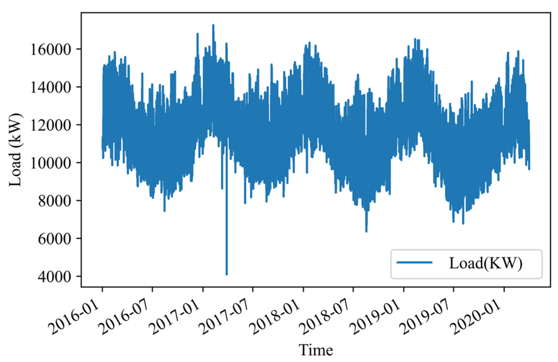
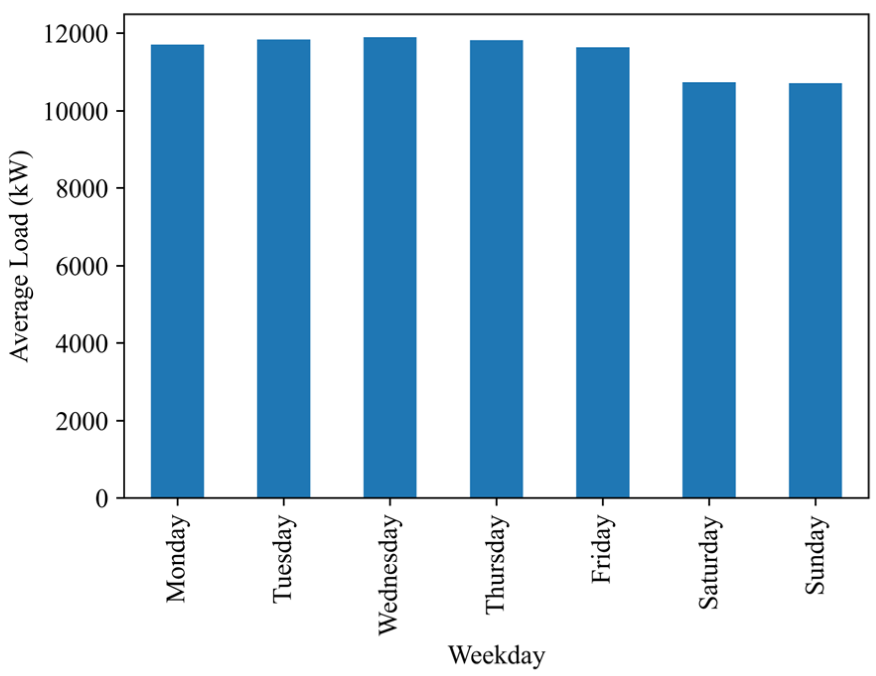
2.1. Campus Load Information

Memorial University of Newfoundland (MUN) is located in St. John’s, Newfoundland and Labrador (NL). The average temperature of the city can range from 6 degrees Celsius to as high as 21 Degrees Celsius. Due to this harsh weather, the heating system represents a very significant portion of the total electric load. MUN employs hot water plants to fulfill its heating requirements. During the harsh weather of winter, the boilers operate at full capacity, while during summer, the load is decreased, and usually half of the boilers are used. The boilers use diesel to operate and can consume up to 70,000 barrels of oil annually to heat more than 50 buildings across the campus. The university uses two meters to monitor the electric load, and meters are used to log data every 15 min. We conduct our analysis using hourly data. Figure 1 is a line plot that shows the trend of electricity consumption for MUN St. John’s campus with a data resolution of 1 h.

The average electric load by weekday can be seen in Figure 2 below. The decreased load during weekends is quite evident. There are minor differences across the week, but a major change is observed in electricity consumption for weekdays and weekends. Understandably, weekdays have a higher consumption of electricity compared to weekends. Figure 3 is a bar plot similar to Figure 2, but it shows the average electricity consumption for each month. Given the weather of St. John’s, it is quite evident that months with higher average temperatures (summer and spring) have a lower electricity consumption compared to months with lower ambient temperatures (winter and fall).

2.2. Metrological Data

Metrological data have a significant impact on energy consumption, so these data are used in the forecasting strategy. Typically used variables for forecasting include temperature, relative humidity, visibility, cloud cover, rainfall, precipitation, dew point, wind speed, and wind chill [19,20]. These metrological data were obtained from weather.gc.ca (accessed on 30 August 2024). Our data use the following metrological factors [14]:

• Dry Bulb Temperature: The temperature visible on a thermometer when it is exposed to the air in the absence of moisture and radiation is called the dry bulb temperature. It is proportional to the mean kinetic energy of the air molecules.
• Dew Point: The temperature required at constant pressure to achieve a relative humidity of 100% is called the dew point of the air. It is directly proportional to the moisture in the air.
• Relative Humidity: At any given temperature, the water mass ratio to air mass represents absolute humidity. The relative humidity is obtained by dividing the absolute humidity by the maximum possible humidity at any given temperature.
• Wind Direction: This represents the direction of the blowing wind. A value of 0 denotes that the wind is calm. A value of 9 represents that the wind is blowing from the east, while a value of 36 means that the wind is blowing from the north.
• Wind Speed: This is the speed of the wind. It is measured at a distance of 10 m from the ground. In our data, we use km/h as the measuring unit.
• Visibility: Visibility is the distance at which an object of tangible size can be observed. In our data, we use kilometers as the measuring unit.
• Atmospheric Pressure: The atmospheric pressure is the force exerted per unit area at the height of the measuring station.

After concatenating metrological and electric data, we obtain our complete training dataset.

Table 1. Comparison of different algorithms.

Research Article	Spatiotemporal Mapping	Robustness Testing	Input Horizon Optimization
[13]	No	No	No
[14]	No	No	No
[15]	Yes	No	No
[16]	Yes	No	No

shows all the chief features of the complete dataset, which are then fed to the preprocessing pipeline.

Table 2. Training dataset parameters.

Parameter	Value
Data start date	2 January 2016
Data end date	31 March 2020
Data interval	1 h
Total data points	37,221
Features	08

shows all the parameters for the training dataset.

3. Algorithms, Evaluation Metrics, and Loss Functions

3.1. Algorithms

3.1.1. Seasonal Autoregressive Integrated Moving Average (SARIMA)

The SARIMA algorithm is the variation of the Autoregressive Integrated Moving Average (ARIMA) algorithm, which handles the seasonality in the data. ARIMA itself is a generalized case of the Autoregressive Moving Average (ARMA) algorithm. An ARIMA algorithm has the following components:

Autoregressive Model: the autoregressive model is a common way to model a time series. Equation (1) represents the time series as an autoregressive model. It means that the future values of a time series are linearly related to the previous values in the time series. The order of the time series represents the number of previous values. For example, if a time series has an autoregressive order of p, then it means that any value in that time series can be written as a linear combination of previous p values. Such a time series would be called an AR(p) time series:

$$y_t=\delta +{\phi }_1{y}_{t-1}+{\phi }_2{y}_{t-2}+\cdots +{\phi }_p{y}_{t-p}+{ϵ}_t$$

(1)

Here, ${ϵ}_t$ represents the white noise. Here, $y_t$ can be seen as a regression p lagging values; hence, it is an AR(p) model.

Moving Average Model: The moving average model is a way to model a time series as a linear combination of past forecasting errors. Equation (2) represents the time series as a moving average model. A moving average model of order q can be represented as MA(q). Each value in such a time series can be thought of as a moving average of past q forecasting errors. This can be observed in Equation (2).

$$y_t=\mu +{ϵ}_t-{\epsilon }_{t-1}{\theta }_1-\cdots -{\epsilon }_{t-q}{\theta }_q$$

(2)

Here, $\mu$ represents the mean. (${ϵ}_t$,…${\epsilon }_{t-q}$) represent the past errors, while (${\theta }_1$…${\theta }_q$).

An ARIMA model is obtained by combing these two models with differencing to induce stationarity on the time series. The order of differencing is represented by the parameter d. Hence, the ARIMA(p,d,q) model is represented by three parameters, i.e., p,d, and q, each representing the order of autoregression, differencing, and moving average of the model.

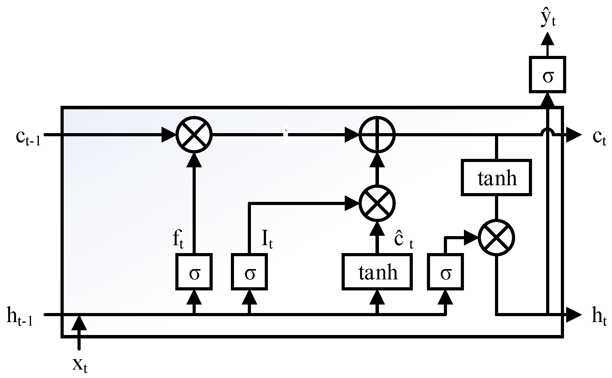
3.1.2. Long Short Term Memory Recurrent Neural Network

Recurrent neural networks are a type of artificial neural network that are capable of handling sequential data. A simple RNN network takes the input value of the sequence and combines it with the hidden state from the previous timestamp and uses an activation function to generate the hidden state for the next timestamp. RNNs are susceptible to exploding and vanishing gradients. To resolve this issue, RNN cells are modified using various gates. The Long Short Term Memory (LSTM) [21] artificial neural network consists of LSTM cells, and each cell has an input gate, output gate, and forget gate. Through these gates, an LSTM cell can forget or pay attention to different parts of a sequential input [22].

Forget Gate: The forget gate ($f_t$) determines what data need to be forgotten from a network’s long-term memory/cell state ($c_t$) based on the new input $x_t$ and hidden state obtained from the previous time step ($h_{t-1}$).

$$f_t=sigmoid\left(W_{fx}{x}_t+W_{fh}{h}_{t-1}+b_f\right)$$

(3)

Input Gate: The input gate ($I_t$) determines which information needs to be added to the network based on the current input and hidden state from the previous step. The gate also generates a candidate hidden state (${\widehat{c}}_t$) by using a tangent hyperbolic activation function. Finally, the cell state at time $t$ represented by $c_t$ is calculated as well:

$$I_t=sigmoid\left(W_{Ix}{x}_t+W_{Ih}{h}_{t-1}+b_I\right)$$

(4)

$${\widehat{c}}_t=tanh\left(W_{cx}{x}_t+W_{ch}{h}_{t-1}+b_c\right)$$

(5)

$$c_t=f_t.c_{t-1}+{\widehat{c}}_t.I_t$$

(6)

Output Gate: The output gate ($O_t$) generates the hidden state ($h_t$), which is passed over to the next LSTM cell.

$$O_t=sigmoid\left(W_{ox}{x}_t+W_{oh}{h}_{t-1}+b_o\right)$$

(7)

$$h_t=O_t\otimes tanh(c_t)$$

(8)

All the variables represented by $W$ and $b$ represent weights and biases (respectively) learned by the network during training. The $\otimes$ symbol represents pointwise multiplication. Figure 4 shows a basic LSTM unit below.

3.1.3. Gated Recurrent Unit

Gated Recurrent Units are a type of recurrent neural network in which a single unit has 2 gates (reset gate and update gate) [23]. GRUs also do not have cell states and instead, they use hidden states to pass the information to the next time step. Compared to LSTMs, this network is simpler and takes less time to train. A basic GRU unit is shown in Figure 5.

The basic description of the gates is given below:

Reset Gate: The reset gate decides how much of the previous information needs to be forgotten.

$$r_t=sigmoid\left(W_{rx}{x}_t+W_{rh}{h}_{t-1}+b_r\right)$$

(9)

Update Gate: The update gate in the GRU decides how much of the information from previous time steps need to be passed to the next blocks.

$$z_t=sigmoid\left(W_{zx}{x}_t+W_{zh}{h}_{t-1}+b_z\right)$$

(10)

First, the reset gate is used to create a candidate vector (${\widehat{h}}_t$) while following

$${\widehat{h}}_t=tanh\left(W_z{x}_t+W_h(r_t\otimes h_{t-1})+b_{ht}\right)$$

(11)

Finally, the update gate is used to generate the hidden state as follows:

$$h_t=z_t\otimes {\widehat{h}}_t+\left(1-z_t\right)\otimes h_{t-1}$$

(12)

3.1.4. Bi-Directional Recurrent Neural Networks

Bi-directional RNNs process the data in both directions using two separated hidden layers before feeding them to the same output layer [24]. This architecture can be used for both LSTM Recurrent Neural Networks (Bi-Directional LSTM) and Gated Recurrent Networks (Bi-Directional GRU).

3.1.5. Convolutional Neural Network

Convolutional neural networks (also referred to as shift invariant artificial neural networks) consist of filters that slide along the input features to create feature maps. Typical convolutional neural network architectures usually consist of convolutional layers with a pooling layer between two convolutional layers and dense or fully connected layers.

A convolutional layer performs convolutional operations using filters or kernels to generate feature maps. Important parameters include the stride and filter size. Each neuron of a feature map is connected to neurons in the previous layer, referred to as the receptive field of that neuron.

The activation value of a neuron located at the (i,j) location in the kth feature map of layer l is obtained by passing the feature map through an activation function, which adds the ability to learn non-linear patterns to a network. The activation value can be represented as

$$a_{i,j,k}^l={Activation(W_k^l}^T{x}_{i,j}^l+B_h^l)$$

(13)

Here, $x_{i,j}^l$ represents the input, while ${W_k^l}^T$ and $B_h^l$ are weights and biases. Activation functions used could be ReLU, tanh, or sigmoid.

Pooling operation is used to sample the feature map. It introduces shift invariance to the network. Max pooling [25] and average pooling [26] are the typical pooling operations employed in convolutional networks. Pooling layers are placed between two convolutional layers.

A network usually consists of a number of convolutional layers with pooling layers in between. The earlier layers in a network learn low-level features, while the layers after learn more abstract or higher-level features. In the case when a convolutional neural network is used for image classification, the earlier layers will learn features such as lines, edges, and corners, while later layers learn more abstract features that are built on top of previous low-level features.

After several convolutional and pooling layers, one or more fully connected layers are added at the end of the network. This fully connected layer performs high-level reasoning, although it can be replaced by a 1x1 convolution layer [27]. This layer is then connected to the output layer. A loss function is generated using the output of this layer and true outputs from the training dataset. This loss function is then minimized to obtain network parameters (weights and bias terms). A popular optimization algorithm used for minimizing loss function is stochastic gradient descent [28].

3.1.6. Sequence to Sequence (Seq2Seq) Model

As the name implies, this model converts an input sequence to an output sequence. The length of both sequences can be different. The model consists of two recurrent neural networks. The input is fed to a network called the encoder network, while we obtain an output from a model called the decoder network.

The encoder model is a recurrent neural network that takes an input sequence. At each time step in the recurrent neural network, the GRU or LSTM block takes the input of that time step and produces an output and a hidden state. The hidden state is passed along to the next LSTM/GRU block, which uses it along with input from that time step to generate a hidden state for the next block. The hidden state generated by the last LSTM/GRU block is used as the initial hidden state for the decoder part. It is called the context vector.

The decoder is an RNN consisting of either GRUs or LSTMs. The first decoder block uses a hidden state to generate output value and a hidden state for the next LSTM/GRU block. Each block will use the output and hidden state from the previous block.

3.1.7. Sequence to Sequence (Seq2Seq) Model with Attention

The motivation for using the attention mechanism stems from the underperformance of the basic encoder–decoder model for long sequences. This is caused by the use of a fixed-length context vector.

When using the attention mechanism, an alignment score is calculated by using a vector consisting of all the encoder hidden state vectors as well as the output generated from the decoder block of the previous time step. Using alignment scores, attention weights are generated using the Softmax Activation function, and finally, a context vector is generated by using attention weights and encoder hidden states.

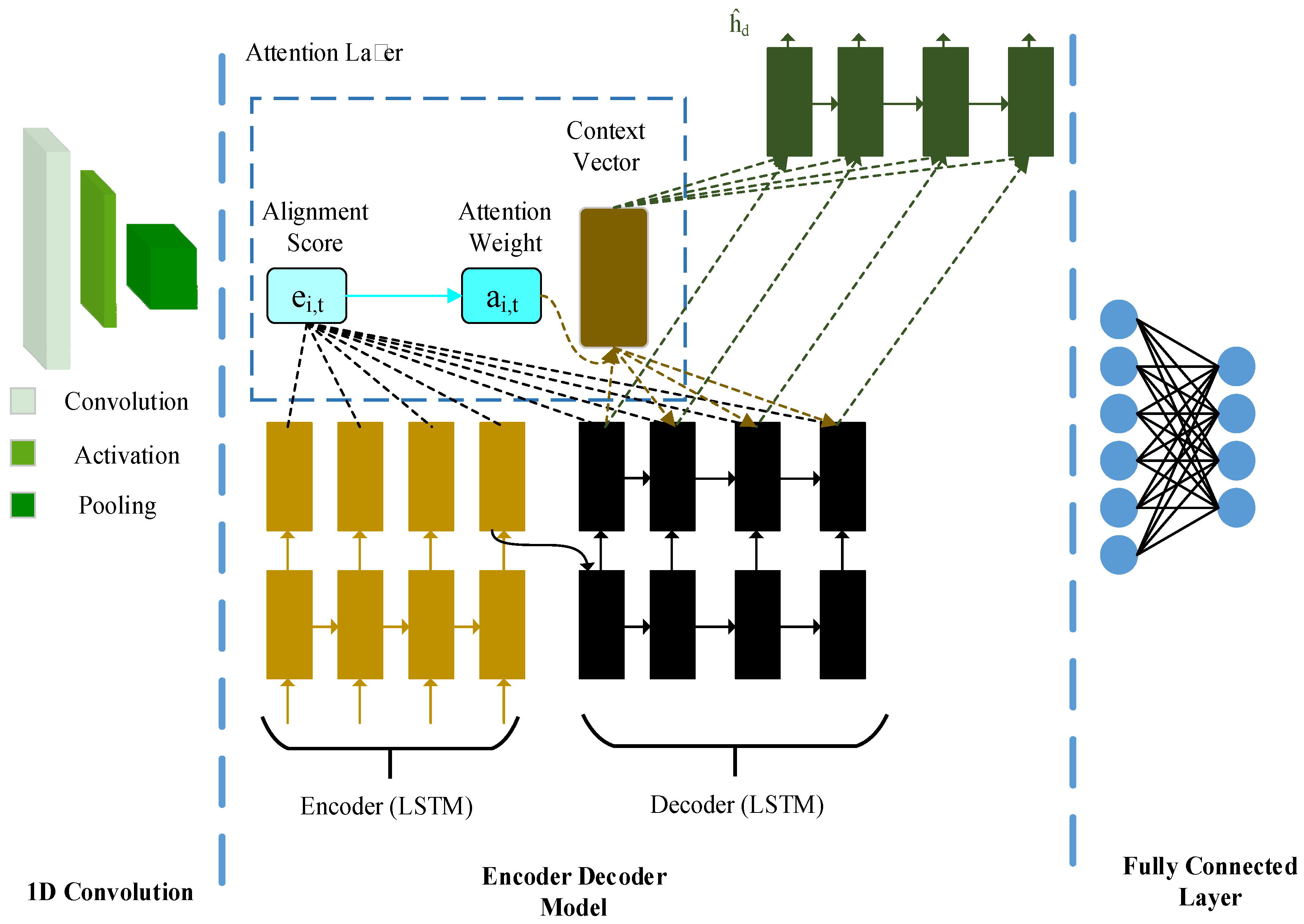
3.1.8. Proposed Custom Architecture

The proposed custom architecture consists of a 1D convolution neural network (CNN). The 1D CNN provides temporal features to the next model, which is the encoder–decoder model. The encoder–decoder model also has an attention mechanism. The attention mechanism helps the encoder–decoder model to pay attention to more important patterns in the extracted temporal features. Both the encoder and decoder consist of GRU units. After the encoder–decoder model, a fully connected layer is used. The 24 output cells of the fully connected layer are the predicted outputs representing the predicted hourly load profile of the model.

3.2. Evaluation Metrics

3.2.1. Mean Absolute Error (MAE)

The mean absolute error is the average of the absolute difference between a predicted/forecasted value and ground truth. It can be written as

$$\mathrm{M}\mathrm{e}\mathrm{a}\mathrm{n} \mathrm{A}\mathrm{b}\mathrm{s}\mathrm{o}\mathrm{l}\mathrm{u}\mathrm{t}\mathrm{e} \mathrm{E}\mathrm{r}\mathrm{r}\mathrm{o}\mathrm{r}={\displaystyle \frac{{\sum }_{i=1}^N\left|P_i-G_i\right|}{N}}$$

(14)

Here, $P$ and $G$ are predictions and ground values, respectively. $N$ is the number of values in the dataset. If an estimator is more accurate, it results in a lower MAE. An inaccurate estimator results in a higher MAE. One major drawback of the MAE is that it is scale-dependent (it uses same scale as that of the dataset). Being scale-dependent means that it cannot be used to compare algorithm performance across different datasets.

3.2.2. Mean Squared Error

The mean squared error is the average of the squared difference between the predicted values and ground truth. This evaluation metric is based on Euclidean distance. It can be written as

$$\mathrm{M}\mathrm{e}\mathrm{a}\mathrm{n} \mathrm{S}\mathrm{q}\mathrm{u}\mathrm{a}\mathrm{r}\mathrm{e}\mathrm{d} \mathrm{E}\mathrm{r}\mathrm{r}\mathrm{o}\mathrm{r}={\displaystyle \frac{{\sum }_{i=1}^N({P_i-G_i)}^2}{N}}$$

(15)

This evaluation metric is based on the Euclidian distance. An accurate estimator would have a lower MSE, while an inaccurate estimator would have a higher MSE. Compared to MAE, MSE is more sensitive to outliers since errors are squared. MSE is scale-dependent, so it should only be used to compare algorithm performance for the same dataset.

3.2.3. R² Score

This is also referred to as the coefficient of determination. It can have a maximum value of 1, which would indicate that the model has predicted every ground truth value correctly. It can also have negative values with no limit since an estimator can be arbitrarily worse. If the ground truth is non-constant and the model predicts a constant mean value, then the R² value would be 0. The formula for this metric is given by the relationship below:

$$R^2=1-{\displaystyle \frac{{\sum }_{i=1}^N({P_i-G_i)}^2}{{\sum }_{i=1}^N({G_i-M)}^2}}$$

(16)

Here, M is the mean of all the observed values and is defined as

$$M=\sum _{i=1}^N\left(G_i\right)$$

(17)

It is evident from 15 that the $R^2$ would have a value of 1 for a model with all the predicted values equal to ground truths, as $({P_i-G_i)}^2$ would be 0. For a baseline model that only predicts mean values, ${\displaystyle \frac{{\sum }_{i=1}^N({P_i-G_i)}^2}{{\sum }_{i=1}^N({G_i-M)}^2}}$ would be 1, and the overall value would be 0. Adding a high number of features to the model can increase the R² score of the model, even though it might have lower prediction power. Similarly, a model with non-random residuals can have high score while still being fairly inaccurate. So, it is always advisable to use the coefficient of determination with other metrics, such as the mean squared error, mean absolute error, and mean absolute percentage error.

3.2.4. Mean Absolute Percentage Error (MAPE)

The mean absolute percentage error (MAPE) is an evaluation metric that is defined as

$$\mathrm{M}\mathrm{A}\mathrm{P}\mathrm{E}={\displaystyle \frac{100}{n}}\sum _{i=1}^N\left|{\displaystyle \frac{{G_i-P}_i}{G_i}}\right|$$

(18)

This metric is independent of the scale of data and can be used to compare an algorithm across different time series. However, if a time series has zero or near zero values, this evaluation metric becomes infinite. It also penalizes negative and positive errors asymmetrically. A more accurate algorithm would have a lower MAPE compared to a less accurate model.

4. Methodology and Results

4.1. Methodology

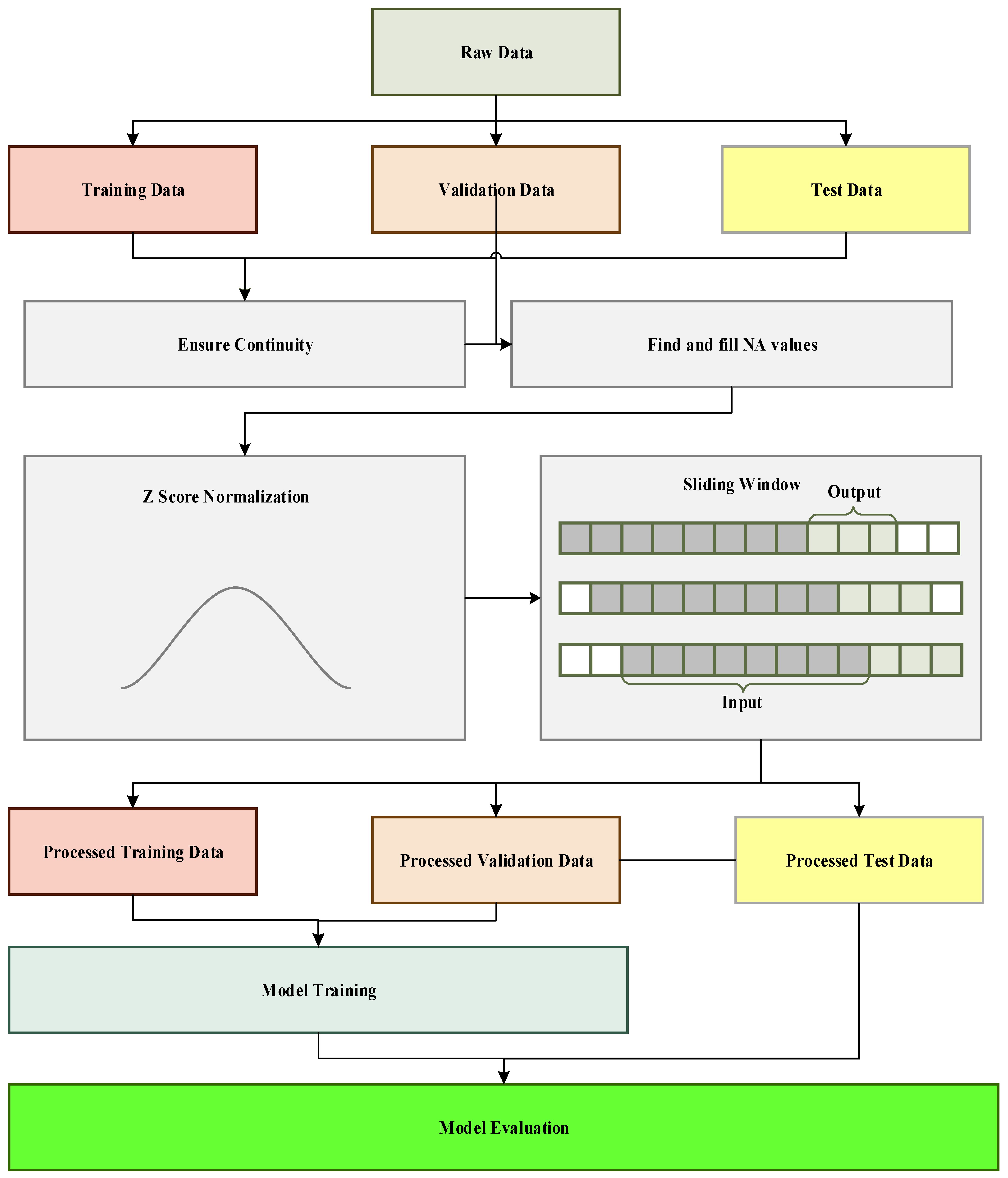
4.1.1. Data Cleaning

Data cleaning and data preprocessing are divided into two different steps as they represent different sets of procedures used on the dataset. Typically, data cleaning consists of initial set of methods, while data preprocessing occurs downstream of data cleaning and involves more advanced techniques.

Data cleaning is performed on the data to make it consistent and remove any discrepancies. Some of the major data cleaning procedures involve the following:

Removal of outliers could be extremely large values, extremely small values, or non-plausible values (such as negative values for temperature in Kelvin). They might be a part of the dataset because of a number of reasons, including faulty instrument or some errors in data-collection software.

Removal of any NA (Not available) values from the dataset. These values represent gaps or breaks in the data.

The outliers are detected based on interquartile range (IQR). These outliers are then represented as NA values. These NA values along with any gaps in the dataset are filled using forward-filling method. This method involves filling any breaks or outliers in the data with values from previous timestamp. Data were analyzed again to find any missing values and outliers. None were found after the procedure.

4.1.2. Data Preprocessing

In this step, data standardization is performed. Data standardization is carried out for each feature separately. This process helps the model converge faster. It is also called Z-Score Normalization. It is more robust to any outliers in the data compared to data normalization. Equation (19) shows the basic formula for the standardization of a single feature.

$$x_{normalized}={\displaystyle \frac{x-M}{\alpha }}$$

(19)

Here, α is the standard deviation.

Secondly, a sliding windowing function is implemented. Data windowing is performed to create input–output pairs from a continuous time series. Since we are using the hourly input, we will be dividing the time series into continuous slices while striding 24 time steps, which correspond to one complete day. The output of the network is an hourly prediction of one complete day.

After data windowing, we divide the dataset into 3 portions. These are the training set, validation set, and test set. A total of 75% of the data is used for training and 15% is used for validation, while remaining 10% of the data is used for testing.

4.1.3. Network Architecture

The networks used for training include RNNs (LSTM and GRU), a 1D CNN + encoder–decoder model, as well as a custom architecture consisting of a 1D CNN followed by an encoder–decoder model with attention. The difference between the above 2 models is the attention mechanism. Following this, a fully connected layer generates the desired output. The complete model pipeline is shown in Figure 6 while the proposed architecture is shown in Figure 7.

Model consists of three main parts. The first part is the 1D CNN model, which aims to embed the spatial features in the model. These features include metrological features present in the original data. The second part is the RNN network based on LSTM model. This portion of the model is concerned with temporal features of the data. The dataset is fed to network in the form of windows, so LSTM model tries to capture the temporal patterns and features in the data. Finally, we have the attention mechanism, which is part of the temporal network. Attention mechanism is typically used for capturing long-range dependencies. Here, this mechanism captures long-range temporal features that could be missed by a simple RNN or LSTM.

4.1.4. Training

Finally, the training set is used to train the data. Huber loss is used along with Adams optimizer.

$$Huber loss=\left\{\begin{array}{c}{\displaystyle \frac{1}{2}}{\left(P-G\right)}^2 for \left(P-G\right)\le \delta \\ \delta . \left(\left|P=G\right|-{\displaystyle \frac{1}{2}}\delta \right), otherwise\end{array}\right.$$

(20)

Equation (20) defines the Huber loss. This loss function is non-linear (quadratic) for small values of the residual (P-G) and linear for larger residuals. As a result, this function combines the sensitivity of mean squared error (MSE) with the robustness of mean absolute error (MAE).

Each of the algorithms is trained up to 100 epochs. An early stopping routine is implemented for a more efficient training process and to save time. Validation loss is monitored, and the best results are saved based on its minimum value.

Table 3. Training hyperparameters.

Hyperparameters	Values
Epochs	100
Loss Function	Huber Loss
Batch Size	128
Optimizer	Adams Optimizer
Early Stopping Patience	20
Early Stopping Parameter	Validation Loss
Input Features	10
Output Window Width	24
Input Window Width	672

shows the training hyperparameters. Finally, mean absolute error (MAE), mean squared error (MSE), mean absolute percentage error (MAPE), and R² values are tabulated on the test data to evaluate the model performance.

Table 4. Training and Inference time.

Parameter	Value (Seconds)
Training time	257.4
Inference time	0.21

shows training and inference times on Nvidia GTX 970m (Santa Clara, CA, USA) and Intel i7 4720 HQ (Santa Clara, CA, USA) with 16 GB of memory for the model with best performance.

4.2. Results

4.2.1. Model Comparison

Data cleaning and preprocessing were performed in Python 3.9 using pandas and Numpy. Keras was used to create deep learning models and compare various evaluation metrics. We can see graphs of electric load prediction created by all the models. By looking at the prediction graphs in Figure 8, it can be seen that the models have learned the daily electric usage profile quite well. The proposed model has the lowest MAPE, MSE, and MAE. The proposed model also shows the highest R² score. We also compare this to some of the other forecasting models found in literature, which include Rational Quadratic Gaussian Process Regression (RQ-GPR), which is used in [12] for interpolation; however, we are interested in forecasting future values while training the model on past information. We compare our model with this algorithm. Similarly, model proposed in [14], called sequence to sequence + Luong attention, is also trained and compared with our trained algorithm. RQ-GPR has the weakest performance compared to all the other algorithms, as it is a conventional machine learning technique, compared to rest of the methods, which employ deep learning. GRU-based RNN is the second weakest performer, followed by LSTM. Using 1D CNN + sequence to sequence model significantly improves the performance. Adding Luong attention, as mentioned in [14], improves the performance further, but the best performance is achieved by employing the proposed method, which shows lower MAPE, MSE, and MAE. It also shows a higher R² score, which corresponds to better forecasting potential compared to rest of the algorithms. The better performance of the proposed method can be characterized as the ability of the algorithm to capture long-range temporal dependencies and also capture the spatial characteristics between different metrological features.

The major parameters for each of the algorithms used are also shown in

Table 5. Results for various algorithms.

Algorithm/Metric	MAE (kW)	R2 Score	MSE (kW2)	MAPE (% Age)	Chief Parameters
LSTM	442.94	0.77	340,026.33	3.64	Hidden units = 64 Dropout = 0.1 Number of layers = 1
GRU	493.72	0.739	386,019.62	4.05	Hidden units = 32 Dropout = 0.05 Number of layers = 1
1D CNN + Encoder Decoder	423.326	0.8011	294,162.21	3.51	Encoder Hidden units = 32 Decoder Hidden Units = 64 Number of layers = 1
RQ-GPR [14]	450.21	0.71	401,264.54	4.98	Length Scale = 1.0 Scale mixture parameter = 5.0 Noise level range = [0.1, 1]
Sequence to Sequence + Luong Attention [16]	410.11	0.795	298,765.45	3.40	Encoder Hidden Size = 32 Decoder Hidden Size = 64 Attention Layer Hidden Size = 16
Proposed Network Architecture	407.308	0.805	287,346.33	3.37	Encoder Hidden Size = 32 Decoder Hidden Size = 32 Attention Layer Hidden Size = 8

, along with relevant evaluation metrics. A thorough hyperparameter-optimization procedure was carried out for each of the algorithms/methods to ensure a fair comparison among them.

4.2.2. Input Horizon Optimization

We obtained all the results for an input window of 672 time steps; 672 time steps correspond to 28 days (24 × 28 = 672). Since the model uses a 1D CNN network, the number of learning variables is independent of the input size of each training example. This allows us to further optimize the model by varying the input horizon. Using a larger input window allows the network to capture more dependencies among variables, but it also reduces the number of training samples we can have. This can lead to overfitting as a more complex model requires more training examples. The use of a 1D CNN-based network allows the optimization of the input horizon without increasing the number of trainable parameters in the network. Another similar architecture with an LSTM-based encoder–decoder is also used for comparison. The input window was changed from 24 to 672 with an interval of 24. This corresponds to the input horizon ranging from 1 to 28 days. The results are tabulated in

Table 6. Different input horizons.

Architecture	Train Steps	MSE kW2	MAE kW	R2 Score	MAPE (×100%)
GRU	24	536,352.076	541.330	0.663	0.045
	48	464,480.438	501.336	0.708	0.043
	.	.	.	.	.
	.	.	.	.	.
	168	328,631.031	435.952	0.786	0.037
	192	284,889.734	408.822	0.814	0.034
	216	287,705.298	412.394	0.812	0.035
	.	.		.	.
	.	.	.	.	.
	.	.	.	.	.
	648	364,983.889	458.885	0.754	0.038
	672	385,770.860	471.314	0.739	0.039
LSTM	24	508,925.840	533.137	0.680	0.045
	48	488,299.198	532.989	0.693	0.045
	.	.	.	.	.
	.	.	.	.	.
	168	344,335.384	448.178	0.776	0.038
	192	356,604.350	465.067	0.767	0.039
	216	345,513.005	452.298	0.775	0.038
	240	302,698.183	421.951	0.802	0.035
	264	400,005.317	477.321	0.738	0.040
	.	.	.	.	.
	.	.	.	.	.
	648	413,153.544	505.153	0.721	0.042
	672	368,893.385	473.734	0.751	0.039

. The evaluation metrics used are MAPE, MAE, MSE, and R² score. It can be observed from the table below that the GRU-based proposed model performs the best overall with an 8-day (or 192 time steps) input horizon.

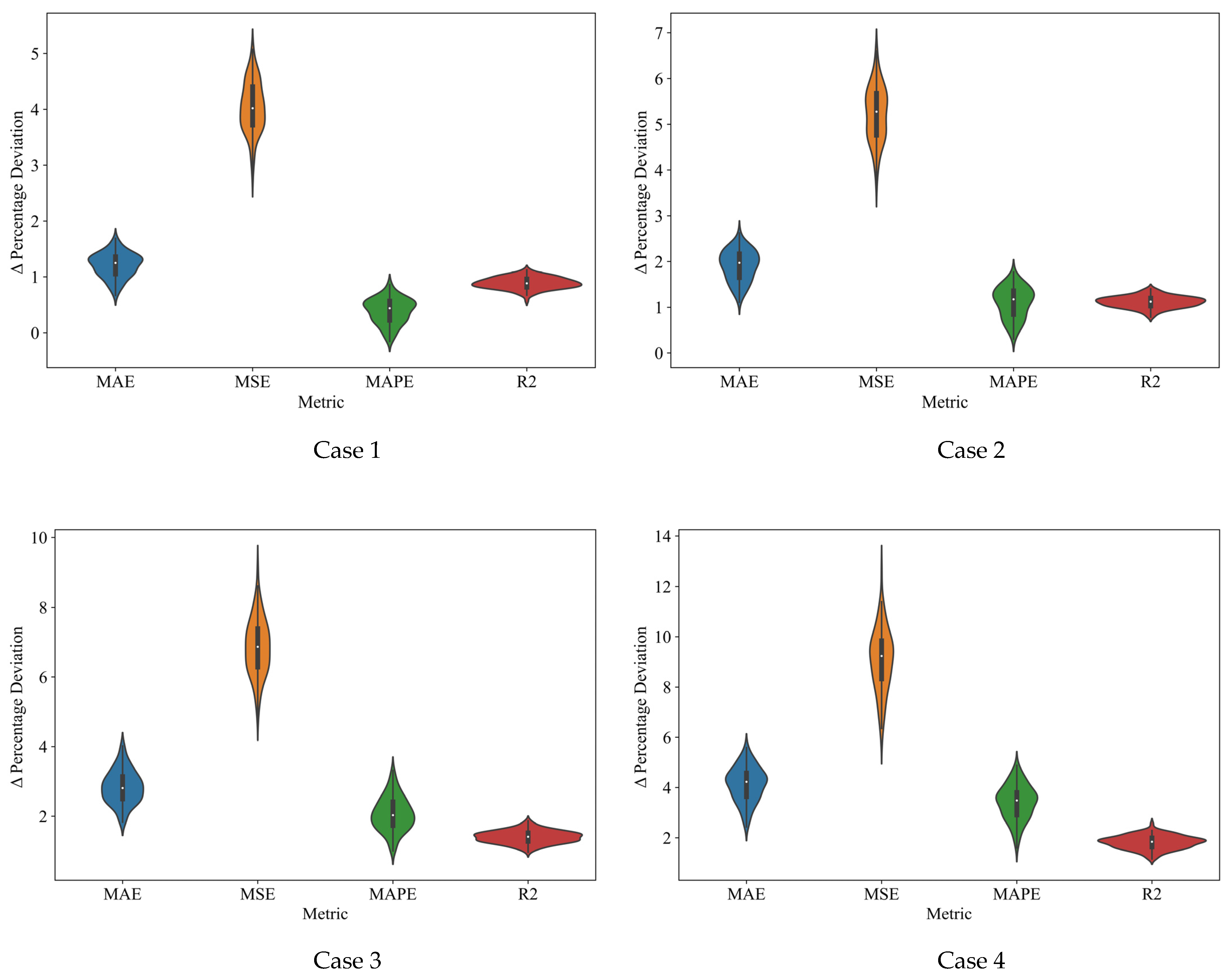
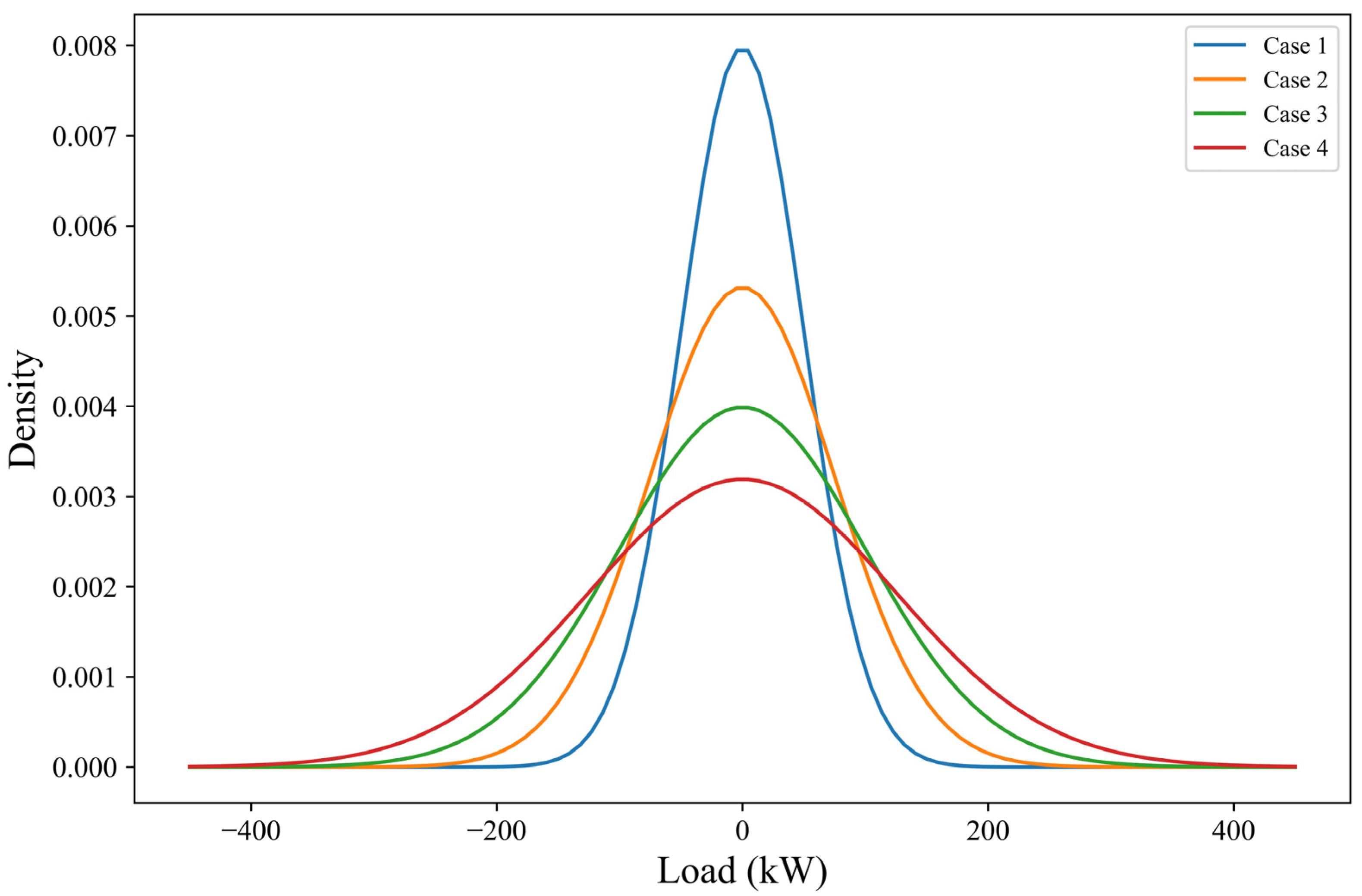
4.2.3. Robustness Testing

To ensure that the trained algorithm is sufficiently robust and invariant to perturbations in the data, noise is added to the testing set, and evaluation metrics are re-evaluated to check for any major changes. Gaussian White Noise is added to the load variable in the data, with a 0 mean and different standard deviations.

Cases are studied with over 100 tests for each case. A case is defined as [μ,σ], where σ is the standard deviation of the normal distribution of the added noise.

Figure 9 shows the basic robustness-testing pipeline. Figure 10 shows the results obtained while Figure 11 shows the probability distribution functions of the 4 cases studied of added noise. These results obtained after conducting over 100 tests are tabulated in

Table 7. Robustness testing with different cases.

Case	Study Details	Test Parameters	Evaluation Metrics
			% ∆MAE	% ∆MSE	% ∆MAPE	% ∆R2
1	[0, 50]	Average	1.241453	4.06674	0.417076	0.89951
		Maximum	1.863907	5.261097	1.003151	1.157584
		Standard Deviation	0.283457	0.509466	0.285956	0.112588
2	[0, 75]	Average	1.85939	5.20309	1.051538	1.111195
		Maximum	2.71684	6.87143	1.879937	1.437032
		Standard Deviation	0.393231	0.663161	0.397011	0.13982
3	[0, 100]	Average	2.796778	6.779848	2.024935	1.405992
		Maximum	4.115265	9.339956	3.419123	1.944015
		Standard Deviation	0.546864	0.948765	0.559865	0.203264
4	[0, 125]	Average	4.02232	8.966153	3.297807	1.807394
		Maximum	5.781688	12.74125	5.005656	2.662423
		Standard Deviation	0.624861	1.205047	0.629848	0.268467

. The highest percentage deviation was observed for MSE, which was close to 12%; this can be explained by the fact that any outliers in the added noise would have affected the score in a more significant manner compared to MAE, MAPE, and the R² score. The rest of the metrics show a maximum deviation of around 6%. The average percentage deviation of the metrics scores also does not exceed 9% (for MSE). Overall, the model is fairly unaffected by the added noise.

5. Conclusions

The model is trained on real-world data and shows a higher R² score and lower MSE, MAE, and MAPE compared to other conventional LSTM-based and GRU-based models. The difference in performance achieved by the attention mechanism is also evident, as the model with attention performs better (a higher R² and lower MAE, MSE, and MAPE) compared to the similar model without attention. An analysis was also carried out to find optimal input window sizes while also changing the basic RNN block from GRU to LSTM. The input window size of 8 days or 192 timse steps with a GRU-based encoder–decoder performs the best, with the lowest MAE and MAPE and the highest R² score. Robustness testing of the proposed method was also conducted and shows that the proposed model is unaffected by the added perturbations to the data.

References

1. Mamun, A.A.; Sohel, M.; Mohammad, N.; Sunny, M.S.H.; Dipta, D.R.; Hossain, E. A Comprehensive Review of the Load Forecasting Techniques Using Single and Hybrid Predictive Models. IEEE Access 2020, 8, 134911–134939. [Google Scholar] [CrossRef]
2. Bashari, M.; Rahimi-Kian, A. Forecasting Electric Load by Aggregating Meteorological and History-Based Deep Learning Modules. In Proceedings of the 2020 IEEE Power & Energy Society General Meeting (PESGM), Montreal, QC, Canada, 2 August 2020; pp. 1–5. [Google Scholar]
3. Zhang, W.; Chen, Q.; Yan, J.; Zhang, S.; Xu, J. A Novel Asynchronous Deep Reinforcement Learning Model with Adaptive Early Forecasting Method and Reward Incentive Mechanism for Short-Term Load Forecasting. Energy 2021, 236, 121492. [Google Scholar] [CrossRef]
4. Chen, J.; Zhao, Y.; Wang, M.; Wang, K.; Huang, Y.; Xu, Z. Power Sharing and Storage-Based Regenerative Braking Energy Utilization for Sectioning Post in Electrified Railways. IEEE Trans. Transp. Electrif. 2024, 10, 2677–2688. [Google Scholar] [CrossRef]
5. Yang, Z.; Yang, Z.; Xia, H.; Lin, F. Brake Voltage Following Control of Supercapacitor-Based Energy Storage Systems in Metro Considering Train Operation State. IEEE Trans. Ind. Electron. 2018, 65, 6751–6761. [Google Scholar] [CrossRef]
6. Mocanu, E.; Nguyen, P.H.; Gibescu, M.; Kling, W.L. Deep Learning for Estimating Building Energy Consumption. Sustain. Energy Grids Netw. 2016, 6, 91–99. [Google Scholar] [CrossRef]
7. Lin, Y.; Luo, H.; Wang, D.; Guo, H.; Zhu, K. An Ensemble Model Based on Machine Learning Methods and Data Preprocessing for Short-Term Electric Load Forecasting. Energies 2017, 10, 1186. [Google Scholar] [CrossRef]
8. Hammad, M.A.; Jereb, B.; Rosi, B.; Dragan, D. Methods and Models for Electric Load Forecasting: A Comprehensive Review. Logist. Supply Chain Sustain. Glob. Chall. 2020, 11, 51–76. [Google Scholar] [CrossRef]
9. Bianchi, F.M.; Maiorino, E.; Kampffmeyer, M.C.; Rizzi, A.; Jenssen, R. An Overview and Comparative Analysis of Recurrent Neural Networks for Short Term Load Forecasting. arXiv 2017, arXiv:1705.04378. [Google Scholar]
10. Zheng, J.; Xu, C.; Zhang, Z.; Li, X. Electric Load Forecasting in Smart Grids Using Long-Short-Term-Memory Based Recurrent Neural Network. In Proceedings of the 2017 51st Annual Conference on Information Sciences and Systems (CISS), Baltimore, MD, USA, 22–24 March 2017; pp. 1–6. [Google Scholar]
11. Wang, X.; Tian, W.; Liao, Z. Statistical Comparison between SARIMA and ANN’s Performance for Surface Water Quality Time Series Prediction. Environ. Sci. Pollut. Res. 2021, 28, 33531–33544. [Google Scholar] [CrossRef] [PubMed]
12. Muzaffar, S.; Afshari, A. Short-Term Load Forecasts Using LSTM Networks. Energy Procedia 2019, 158, 2922–2927. [Google Scholar] [CrossRef]
13. Jain, M.; AlSkaif, T.; Dev, S. Are Deep Learning Models More Effective against Traditional Models for Load Demand Forecasting? In Proceedings of the 2022 International Conference on Smart Energy Systems and Technologies (SEST), Eindhoven, The Netherlands, 5 September 2022; pp. 1–6. [Google Scholar]
14. Madhukumar, M.; Sebastian, A.; Liang, X.; Jamil, M.; Shabbir, M.N.S.K. Regression Model-Based Short-Term Load Forecasting for University Campus Load. IEEE Access 2022, 10, 8891–8905. [Google Scholar] [CrossRef]
15. Yi, L.; Zhu, J.; Liu, J.; Sun, H.; Liu, B. Multi-Level Collaborative Short-Term Load Forecasting. In Proceedings of the 2022 25th International Conference on Electrical Machines and Systems (ICEMS), Chiang Mai, Thailand, 29 November 2022; pp. 1–5. [Google Scholar]
16. Aouad, M.; Hajj, H.; Shaban, K.; Jabr, R.A.; El-Hajj, W. A CNN-Sequence-to-Sequence Network with Attention for Residential Short-Term Load Forecasting. Electr. Power Syst. Res. 2022, 211, 108152. [Google Scholar] [CrossRef]
17. Zuo, C.; Wang, J.; Liu, M.; Deng, S.; Wang, Q. An Ensemble Framework for Short-Term Load Forecasting Based on TimesNet and TCN. Energies 2023, 16, 5330. [Google Scholar] [CrossRef]
18. Fan, C.; Nie, S.; Xiao, L.; Yi, L.; Wu, Y.; Li, G. A Multi-Stage Ensemble Model for Power Load Forecasting Based on Decomposition, Error Factors, and Multi-Objective Optimization Algorithm. Int. J. Electr. Power Energy Syst. 2024, 155, 109620. [Google Scholar] [CrossRef]
19. Jawad, M.; Nadeem, M.S.A.; Shim, S.-O.; Khan, I.R.; Shaheen, A.; Habib, N.; Hussain, L.; Aziz, W. Machine Learning Based Cost Effective Electricity Load Forecasting Model Using Correlated Meteorological Parameters. IEEE Access 2020, 8, 146847–146864. [Google Scholar] [CrossRef]
20. Schaeffer, R.; Szklo, A.S.; Pereira de Lucena, A.F.; Moreira Cesar Borba, B.S.; Pupo Nogueira, L.P.; Fleming, F.P.; Troccoli, A.; Harrison, M.; Boulahya, M.S. Energy Sector Vulnerability to Climate Change: A Review. Energy 2012, 38, 1–12. [Google Scholar] [CrossRef]
21. Hochreiter, S.; Schmidhuber, J. Long Short-Term Memory. Neural Comput. 1997, 9, 1735–1780. [Google Scholar] [CrossRef] [PubMed]
22. Yamak, P.T.; Yujian, L.; Gadosey, P.K. A Comparison between ARIMA, LSTM, and GRU for Time Series Forecasting. In Proceedings of the Proceedings of the 2019 2nd International Conference on Algorithms, Computing and Artificial Intelligence, Sanya, China, 20 December 2019; pp. 49–55. [Google Scholar]
23. Tao, Q.; Liu, F.; Li, Y.; Sidorov, D. Air Pollution Forecasting Using a Deep Learning Model Based on 1D Convnets and Bidirectional GRU. IEEE Access 2019, 7, 76690–76698. [Google Scholar] [CrossRef]
24. Graves, A.; Mohamed, A.; Hinton, G. Speech Recognition with Deep Recurrent Neural Networks. In Proceedings of the 2013 IEEE International Conference on Acoustics, Speech and Signal Processing, Vancouver, BC, Canada, 26–31 May 2013. [Google Scholar]
25. Boureau, Y.-L.; Ponce, J.; LeCun, Y. A Theoretical Analysis of Feature Pooling in Visual Recognition. In Proceedings of the 27th International Conference on Machine Learning, Haifa, Israel, 21–24 June 2010. [Google Scholar]
26. Wang, T.; Wu, D.J.; Coates, A.; Ng, A.Y. End-to-End Text Recognition with Convolutional Neural Networks. In Proceedings of the 21st International Conference on Pattern Recognition (ICPR2012), Tsukuba, Japan, 11–15 November 2012; pp. 3304–3308. [Google Scholar]
27. Gu, J.; Wang, Z.; Kuen, J.; Ma, L.; Shahroudy, A.; Shuai, B.; Liu, T.; Wang, X.; Wang, G.; Cai, J.; et al. Recent Advances in Convolutional Neural Networks. Pattern Recognit. 2018, 77, 354–377. [Google Scholar] [CrossRef]
28. Wijnhoven, R.G.J.; de With, P.H.N. Fast Training of Object Detection Using Stochastic Gradient Descent. In Proceedings of the 2010 20th International Conference on Pattern Recognition, Istanbul, Turkey, 23–26 August 2010; pp. 424–427. [Google Scholar]
Figure 1. MUN electric load.
Energies 17 04457 g001
Figure 2. Average electric load by day.
Energies 17 04457 g002
Figure 3. Average electric load by month.
Energies 17 04457 g003
Figure 4. A basic LSTM unit.
Energies 17 04457 g004
Figure 5. A basic GRU unit.
Energies 17 04457 g005
Figure 6. Model pipeline.
Energies 17 04457 g006
Figure 7. Proposed network architecture.
Energies 17 04457 g007
Figure 8. Predictions for various days using the algorithms.
Energies 17 04457 g008aEnergies 17 04457 g008b
Figure 9. Basic robustness-testing pipeline.
Energies 17 04457 g009
Figure 10. Violin plot showing variation in evaluation metrics for each case.
Energies 17 04457 g010
Figure 11. Probability distribution functions of added noise.
Energies 17 04457 g011