Optimization of Bi-LSTM Photovoltaic Power Prediction Based on Improved Snow Ablation Optimization Algorithm

Abstract

To enhance the stability of photovoltaic power grid integration and improve power prediction accuracy, a photovoltaic power prediction method based on an improved snow ablation optimization algorithm (Good Point and Vibration Snow Ablation Optimizer, GVSAO) and Bi-directional Long Short-Term Memory (Bi-LSTM) network is proposed. Weather data is divided into three typical categories using K-means clustering, and data normalization is performed using the minmax method. The key structural parameters of Bi-LSTM, such as the feature dimension at each time step and the number of hidden units in each LSTM layer, are optimized based on the Good Point and Vibration strategy. A prediction model is constructed based on GVSAO-Bi-LSTM, and typical test functions are selected to analyze and evaluate the improved model. The research results show that the average absolute percentage error of the GVSAO-Bi-LSTM prediction model under sunny, cloudy, and rainy weather conditions are 4.75%, 5.41%, and 14.37%, respectively. Compared with other methods, the prediction results of this model are more accurate, verifying its effectiveness.

1. Introduction

With the rapid development of renewable energy worldwide, photovoltaic (PV) power generation technology has become a hot research topic in the field of new energy [1,2,3]. Unlike the stable grid connection characteristics of traditional fossil energy, PV power generation is significantly influenced by environmental factors such as irradiance, temperature, and humidity. Therefore, conducting research on output power prediction has become a crucial part of the PV power generation process [4]. Accurate prediction of PV power generation can help grid dispatch departments better mitigate risks, facilitate the power sector in making scheduling plans in advance, and reduce the impact of PV grid integration. This is of great importance for the safe and stable operation of the power grid [5,6].

Presently, domestic and international scholars have conducted extensive research into forecasting PV power generation system outputs. Predominant predictive approaches encompass physically modeled mathematical principles as well as data-driven machine-learning algorithms. Physical principle-based mathematical models for PV power generation systems are constrained by factors like installation site specifics and module parameters, thus limiting their applicability for widespread adoption. Conversely, historical-data-based artificial intelligence models exhibit reduced reliance on physical information while demonstrating robust feature extraction capabilities alongside strong generalization potential within diverse datasets. Within artificial intelligence’s predictive methodologies lie three primary categories: traditional direct predictions encompassing support vector machines, Markov-Monte Carlo (MCMC) methods, XG-Boost algorithms, deep-learning techniques comprising BP neural networks along with gate recurrent neural networks (GRU), or long short-term memory neural networks (LSTM); finally, swarm intelligence algorithms integrated with other machine-learning models primarily address issues related to overfitting as well as gradient vanishing or exploding phenomena in singular algorithms.

In the first approach, Al-Duais [7] presents a prediction model that integrates regression analysis and Markov chain processes to enhance prediction accuracy. This is achieved by constructing a state transition probability matrix based on Markov chain theory. Additionally, Zhou et al. [8] validate the effectiveness of the XG-Boost algorithm in power prediction under various weather conditions. Meanwhile, the literature [9,10,11,12] introduces an algorithmic model based on similar day combinations, considering key factors such as season type, weather type, and meteorological conditions. Specific weather conditions of photovoltaic generation are selected for similarity day selection to improve algorithm convergence accuracy. In the second approach, Liu et al. [13] propose a backpropagation BP neural network model and identify the optimal neural network structure as 28-20-11. Furthermore, Castillo-Rojas et al. [14] establish an RNN hybrid architecture capable of effectively processing ordered time series data. Moreover, Wang et al. [15] apply ensemble empirical mode decomposition (EEMD) to decompose original photovoltaic sequence data into high-frequency and low-frequency sub-sequences for feature extraction. An improved LSTM model is then proposed which enhances prediction accuracy and stability by 15% compared with other models. Papers [16,17,18,19,20] utilizing long short-term memory neural networks for predicting PV power generation highlight the need for improvement and optimization of hyperparameters due to unsatisfactory results obtained using traditional long short-term memory neural networks.

In the third approach, Li et al. [21] propose the improved whale optimization algorithm (IWOA) for optimal hyperparameters of Bi-LSTM, and an attention mechanism is incorporated for effective key information capture. Additionally, Lu et al. [22] introduce an improved Grey Wolf Optimization algorithm, integrated with an optimized LSTM neural network, for PV power generation prediction. The approach utilizes cosine similarity, incorporates a non-linear convergence factor, and employs a differential change strategy to enhance the performance of the Grey Wolf Optimization algorithm. The resulting predictive model has demonstrated superiority over traditional GWO optimization strategies. Furthermore, Chen et al. [23] introduce an improved sparrow search algorithm (ISSA) to optimize the hyperparameters of LSTM neural networks for PV power prediction, yielding high prediction accuracy in simulation results. Moreover, Liang et al. [24] propose a prediction model based on decision trees, least squares support vector regression, and an improved whale optimization algorithm for medium-term and short-term PV power prediction at different time scales such as one day prior or a month earlier; this enhances computing speed and prediction accuracy compared to traditional models. Lastly, a PV power forecasting model is developed based on swarm intelligence algorithms combined with other machine-learning models where swarm intelligence optimization algorithms are utilized to optimize parameters of different machine-learning models; results indicate higher prediction accuracy than traditional models along with significant practical value.

This study aims to investigate the latest advancements and research findings in neural network-based PV power forecasting for long-term and short-term memory, analyze the strengths and weaknesses of various swarm intelligence algorithms, and propose an enhanced snow ablation optimization model based on a K-means clustering analysis of weather attributes, categorizing weather into three types: sunny, cloudy, and rainy. By adjusting the hyperparameters of the bipolar long-term and short-term memory neural network, prediction accuracy can be enhanced. Through extensive testing and analysis of real-world data, this study will offer a new theoretical foundation and technical support for PV power generation system forecasting.

2. Data Processing and Analysis

This section delineates the pertinent data analysis procedures subsequent to data acquisition and furnishes relevant data for ensuing model construction.

2.1. Data Processing

The experimental data presented in this paper are derived from the performance test data of the photovoltaic panel group at a specific site of Trina Solar Company, with a sampling interval of 5 min. During this research, the data underwent meticulous preprocessing. Missing values were filled with 0 to guarantee the integrity of the data. Furthermore, to prevent the interference of meaningless data on the model’s prediction results, particularly during the early morning and night when the PV power generation output is typically zero, the data groups with zero PV power generation were excluded from the dataset during the data processing. The time span of the dataset ranges from 15:35 on 14 August 2020 to 23:40 on 27 July 2021. After data processing, the quantity of data decreased from the initial 49,998 to 45,230. To further enhance the prediction accuracy of the model, the data were categorized into three types, namely sunny, cloudy, and rainy, through K-means clustering analysis, corresponding to 14,872, 23,550, and 6,808 data, respectively.

Additionally, during the data division process, strict compliance was maintained with the standard procedures of machine learning. The data was partitioned at a ratio of 3:7, and the models for sunny, cloudy, and rainy conditions were trained and tested respectively. Distinct from the approaches that merely train and test using data from one or two days, this study exploited a substantial amount of data encompassing multiple seasons and weather conditions. This not only strengthened the robustness and generalization capacity of the model but also guaranteed the reliability and practicability of the results. Consequently, the proposed method was not only applicable to the data of one or two specific days but was trained and validated based on an extensive amount of data over an extended period. Such an experimental design renders the research outcomes more valuable for reference.

2.2. Pearson Correlation Coefficient Analysis

Pearson correlation coefficient analysis is a type of statistical method employed to gauge the intensity and direction of a linear association between variables. This paper centers on the degree of influence exerted by environmental variables within the dataset on PV power generation. Different environmental variables might possess varying degrees of influence. Among them, the collected meteorological data encompass environmental information such as global horizontal irradiance (GHI), diffuse horizontal irradiance (DHI), temperature, humidity, wind speed, wind direction, etc. To determine the most significant environmental variable impacting PV power generation, this paper adopts Pearson correlation coefficient analysis to assess the output degree of different environmental variables on PV power generation. The formula of Pearson correlation coefficient is presented as follows:

$$r={\displaystyle \frac{{\displaystyle \sum _{i=1}^n(x_i-\overline{x})(y_i-\overline{y})}}{\sqrt{{\displaystyle \sum _{i=1}^n{(x_i-\overline{x})}^2}}\sqrt{{\displaystyle \sum _{i=1}^n{(y_i-\overline{y})}^2}}}}$$

(1)

Among them, $r$ stands for the Pearson correlation coefficient, which indicates the linear intensity and direction between two variables. In this study, it mainly concerns the relationship between PV power generation and other environmental variables. $x_i$ and $y_i$ are the sample values of the variables. $x_i$ and $y_i$ denote the sample values of the variables. Herein, $y_i$ represents the ith sample value of PV power generation. When the relationship between PV power and GHI is evaluated at this point, $x_i$ stands for the ith observed value of GHI. $\overline{x}$ and $\overline{y}$ respectively denote the sample means of variables x and y. Specifically, $\overline{y}$ represents the sample mean of PV power generation. If the relationship between PV power and temperature is established at this point, then $\overline{x}$ represents the sample mean of temperature.

In addition, $n$ represents the number of samples. Herein, $r$ varies within the range from −1 to 1. A value of 1 indicates a complete positive linear relationship among the variables, while −1 indicates a complete negative linear relationship among the variables. As depicted in Figure 1, it shows the Pearson correlation coefficients between each variable. Power represents the PV power generation value. Among them, the correlation coefficient of GHI is 0.95, the correlation coefficient of wind speed is 0.33, the correlation coefficient of temperature is 0.31, the correlation coefficient of wind direct is −0.095, and the correlation coefficient of humidity is −0.44. Hence, the variable exerting the most significant impact on power is GHI, followed by wind speed and temperature. Humidity also exerts a certain influence, whereas wind direct has nearly no influence on the power generation.

2.3. K-Means Clustering Analysis

The K-means clustering analysis is used to categorize the weather into three types, namely sunny, cloudy, and rainy, in accordance with the attributes of diverse weather conditions such as rainfall and irradiance values. This classification facilitates the establishment of a feature matrix, thereby yielding more standardized training samples, which holds significant importance for enhancing the prediction accuracy of the algorithm. The standardization of the feature matrix enables the algorithm to better learn the patterns under various weather conditions and mitigate the impact of noisy data on model training. Additionally, standardized training samples contribute to improving the generalization ability of the model to ensure that it can handle the PV power prediction under all kinds of weather conditions in practical applications. When undertaking the cluster analysis of weather data, the following indicators should be taken into account to distinguish different weather types:

(1)

The distinction between rainfall weather and other weather conditions can be made based on the quantity of rainfall at different intervals of each day and the occurrence of rain. Herein, the lower threshold is set at 0.5 mm. If the cumulative daily rainfall exceeds 0.5 mm, the weather of that day is classified as a rainy day.

(2)

GHI fluctuation: Sunny days usually have a consistently stable irradiance, resulting in stable and high-power output from photovoltaic modules. Conversely, the movement of clouds in cloudy weather leads to rapid changes in irradiance, thereby causing fluctuations in PV power generation. In this study, the standard deviation of irradiance fluctuation is used as a judgment indicator. If the standard deviation of irradiance exceeds 50 W/m², it is determined as a cloudy day; otherwise, it is determined as a sunny day. The reason for choosing the standard deviation as the evaluation criterion lies in that the standard deviation can effectively measure the degree of dispersion of irradiance values and reflect the magnitude of irradiance fluctuation.

The specific steps of the K-means clustering algorithm are as follows:

(1)

Specify the number of clusters K: Set the number of clusters K for the samples at three, corresponding respectively to the three weather types, namely sunny, cloudy, and rainy. Select three samples from the sample set as the initial cluster centers.

(2)

The Euclidean distance from each data point to the center point of k classes is calculated in turn, and all samples are divided into the nearest class according to the principle of the nearest to the center point of K. The Euclidean distance is:

$$d(x,y)=\sqrt{{\displaystyle \sum _{i=1}^n{(x_i-y_i)}^2}}$$

(2)

(3)

Determines whether the conditions for terminating clustering are met, and if not, returns to step 2. The condition of termination is to meet the following objective function, that is, if the sum of squares of the deviation of each sample to the center point of the class is less than the specified value, and the clustering terminates.

$$\min {\displaystyle \sum _{i=1}^k{\displaystyle \sum _{x_i\in C_i}dist{(C_i,x_i)}^2}}$$

(3)

For each category, there exists a cluster center $C_i$, where i = 1, 2, and 3 respectively correspond to sunny, cloudy, and rainy. Each data point $x_i$ determines its specific category by computing the distances to the three cluster centers. The $dist(C_i,x_i)$ represents the Euclidean distance from data point $x_i$ to $C_i$. The objective of clustering is to minimize the sum of the squared distances from all data points to the corresponding cluster centers, thereby enabling each point to be assigned to the most appropriate weather type. The process analysis diagram is presented as Figure 2.

3. GVSAO-Bi-LSTM Algorithm

This section primarily presents traditional neural network models, such as LSTM neural networks and Bi-LSTM neural networks, along with two enhancement strategies: the Optimal Point Strategy and the Periodic Oscillation Strategy. It provides detailed explanations of the principles behind these two enhancement strategies and simulates the process of snow transitioning from melting to sublimation.

3.1. Good Point Strategy

In the enhancement of optimization algorithms, the initialization stage frequently boosts the overall performance of the algorithm through modifying the random distribution of the population. Conventional approaches typically employ the strategy of randomly generating the population; however, this method readily causes the population to concentrate in specific areas of the parameter space, thereby heightening the risk of the algorithm being trapped in the local optimal solution. To address this issue, this study incorporates the Good Point strategy to optimize the initialization process of the population. The Good Point Strategy is an effective parameter optimization method originally proposed by the Chinese mathematician Hua Luogeng [25]. The core concept lies in searching for the initial points via uniform distribution within the parameter space. In contrast to the traditional random generation approach, Good Point strategy ensures that the initial population uniformly covers the entire parameter space by devising a uniformly distributed scheme. This uniformity enhances the diversity of the population and lowers the probability that the initial points are concentrated in a specific region, thereby effectively preventing the algorithm from getting trapped in the local optimal solution at the early stage. Its basic definition and construction are as follows: Set $G_s$ is a unit cube in $S$ dimensional Euclidean space. The range of each coordinate value’s interval is [0, 1].

$$G_s=\left\{\left(x_1,x_2,\dots ,x_s\right)\mid 0\le x_i\le 1,\forall i=1,2,\dots ,s\right\}$$

(4)

Among them, $x_i$ represents the coordinate on the ith dimension; $S$ is the dimension of the space.

If $r\in G_s$:

$$P_n(k)=\left\{\left\{r_1^{(n)}\cdot k\right\},\left\{r_2^{(n)}\cdot k\right\},\dots ,\left\{r_s^{(n)}\cdot k\right\}\right\}$$

(5)

where n is a positive integer, denoting the quantity of parameters utilized when generating the point set; $k$ is a natural number, signifying the index value of the generated point within the set; $r_i^{\left(n\right)}$ represents the parameter of the ith variable in the nth calculation. Through this operation, the sampling points can be concentrated within the unit cube.

Its deviation $f_{(n)}$ satisfies:

$$f_{(n)}=C(r,\epsilon )n^{-1+\epsilon }$$

(6)

where $C(r,\epsilon )$ is a constant that is only related to $r$ and $\epsilon$, and $\epsilon$ is any positive number, then $P_n(k)$ is the set of good points and $r$ is the good point.

Through the definition and construction of the above three formulas, the good point sets that are uniformly distributed in the parameter space can be effectively generated. These point sets can significantly improve the diversity of the population of the optimization algorithm, thereby enhancing the global search ability of the algorithm and reducing the risk of falling into local optima.

3.2. Vibration Strategy

The Vibration strategy is frequently employed to introduce a certain level of stochasticity or variability into the search process, thereby aiding the algorithm in augmenting its global search capability. The fundamental concept involves introducing random perturbations or variations to the current solution or parameters of the objective function during the iterative optimization process based on a defined periodic function or pattern. In this study, we utilize a sine function oscillation, which serves to modify the position or velocity of the solution. The basic formula is as follows:

$$X_{new}=X_{current}+A\cdot \sin (2\pi \cdot {\displaystyle \frac{k}{T}})$$

(7)

$X_{current}$ represents the current position state, $A$ represents the amplitude, $K$ represents the current iteration count, and $T$ represents the oscillation period.

3.3. Snow Ablation Optimization Algorithm

The snow ablation optimizer (SAO) is a novel optimization algorithm that simulates the melting and sublimation processes of snow. This algorithm achieves a balance between exploration and exploitation in the solution space, thereby avoiding premature convergence and making it suitable for complex global optimization problems. The inspiration for the SAO algorithm comes from the physical changes in snow found in nature, including sublimation and melting. As shown in Figure 3, the sublimation process involves snow transitioning directly from a solid to a gaseous state under low-temperature and low-pressure conditions, simulating large jumps in the solution space and promoting extensive exploration. The melting process involves snow transitioning from a solid to a liquid state as the temperature increases, simulating local searches in the solution space and aiding in finding local optima. The core of the algorithm is to balance global exploration and local optimization by simulating the physical changes in snow.

The specific principle includes the initialization stage, the exploration stage, and the exploitation stage [26]. In the initialization stage, the iterative process typically commences with a population randomly generated. The randomly generated population is capable of covering diverse regions of the solution space, thereby facilitating the guarantee that the algorithm does not prematurely fall into local optima and enabling it to explore a broader solution space. Generally, the entire population is modeled as a matrix with the population size and the dimension of the solution space, as depicted in the following equation, where N represents Population 1 and Dim represents the dimension of the solution space.

$$Z={\left[\begin{array}{ccccc}{z}_{1,1}& z_{1,2}& \cdots & z_{1, \mathrm{Dim}-1 }& z_{1, \mathrm{Dim} }\\ z_{2,1}& z_{2,2}& \cdots & z_{2, \mathrm{Dim}-1 }& z_{2, \mathrm{Dim} }\\ ⋮& ⋮& ⋮& ⋮& ⋮\\ z_{N-1,1}& z_{N-1,2}& \cdots & z_{N-1, \mathrm{Dim}-1 }& z_{N-1, \mathrm{Dim} }\\ z_{N,1}& z_{N,2}& \cdots & z_{N, \mathrm{Dim}-1 }& z_{N, \mathrm{Dim} }\end{array}\right]}_{N\times \mathrm{Dim} }$$

(8)

In the exploration stage, when snow is transformed from solid to liquid and finally into steam, Brownian motion can effectively simulate the diffusion of steam in the search space due to its dynamic and uniform step size characteristics. Therefore, Brownian motion is used to simulate this random process. The main process is as follows:

$$\begin{array}{l}{Z}_i\left(t+1\right)=Elite\left(t\right)+B{M}_i\left(t\right)\otimes \\ \left({\theta }_1\times \left(G\left(t\right)-Z_i\left(t\right)\right)+\left(1-{\theta }_1\right)\times \left(\overline{Z}\left(t\right)-Z_i\left(t\right)\right)\right)\end{array}$$

(9)

$$Elite(t)\in \left[G\left(t\right),Z_{\sec ond}\left(t\right),Z_{third}\left(t\right),Z_c\left(t\right)\right]$$

(10)

$$\overline{Z}\left(t\right)={\displaystyle \frac{1}{N}}{\displaystyle \sum _{i=1}^N{Z}_i\left(t\right)}$$

(11)

$$Z_c\left(t\right)={\displaystyle \frac{1}{N_1}}{\displaystyle \sum _{i=1}^{N_1}{Z}_i\left(t\right)}$$

(12)

where: $Z_i\left(t\right)$ indicates the position of the $i$ molecule at time $t$; $B{M}_i\left(t\right)$ represents a random number vector based on Gaussian distribution and used to describe Brownian motion; $G\left(t\right)$ indicates the current optimal solution; $Elite\left(t\right)$ represents an elite individual randomly selected from the group; ${\overline{Z}}_{\left(t\right)}$ represents the solution of the centroid position of the whole group; $Z_{\sec ond}\left(t\right)$, and $Z_{third}\left(t\right)$ represents the second and third best solutions in the current population, respectively. $Z_{c\left(t\right)}$ indicates the individual centroid position solution with fitness in the top 50%. The weighting factor, represented by ${\theta }_1$, is employed to balance the influence exerted by $G\left(t\right)$ and ${\overline{Z}}_{\left(t\right)}$ on the individual update.

It can be discerned from the formula for the updated positions of molecules that the principle of position update lies in delineating the computation of the tensor product of the cross-terms and random vectors of Brownian motion. These two vectors delineate the cross-terms of the two-dimensional parameter space. Among them, the first vector governs the movement towards the current best individual, while the second vector governs the movement towards the centroid. The two cross-terms predominantly describe the interaction among individuals.

During the development stage, the search process is predominantly governed by introducing the key parameter of snowmelt rate, allowing the algorithm to strike a balance between global search and local optimization. Additionally, the modulation of the snowmelt speed not only mirrors the inspiration source of the actual physical process but also precisely delineates this dynamic change through mathematical formulations, guaranteeing the coherence of the algorithm in both theory and practice. The snowmelt rate is dynamically adjusted in accordance with the temperature, emulating the gradual alteration of the actual snowmelt process. When the snow transforms into liquid water, the degree-day method is employed to depict this behavior:

$$M=DDF\times \left(T-T_1\right)$$

(13)

$$DDF=0.35+0.25\times {\displaystyle \frac{e^{\frac{T}{T_{\max }}}-1}{e-1}}$$

(14)

where $DDF$ represents the degree-day factor, which is used to estimate the amount of snow ablation. $T$ represents the current temperature. $T_{\max }$ denotes the maximum temperature recorded during a specific time interval. $T_1$ indicates the base temperature. Therefore, in the update phase, the position update equation is as follows:

$$\begin{array}{l}{Z}_i\left(t+1\right)=M\times G\left(t\right)+B{M}_i\left(t\right)\otimes \\ \left({\theta }_2\times \left(G\left(t\right)-Z_i\left(t\right)\right)+\left(1-{\theta }_2\right)\times \left(\overline{Z}\left(t\right)-Z_i\left(t\right)\right)\right)\end{array}$$

(15)

At time $t+1$, $Z_i\left(t+1\right)$ denotes the position of the ith individual; $M$ represents the scaling factor, which is utilized to adjust the impact of $G\left(t\right)$ on the individual’s updated position; and ${\theta }_2$ is the weight factor used to balance the movement of the individual between $Z_i\left(t\right)$ and $G\left(t\right)$.

3.4. Bi-LSTM Neural Network Model

Bi-LSTM is a variant of LSTM that combines both forward and backward LSTM structures. Substructures allow the network to consider both past and future information when processing sequence data, better capturing the semantics and dependencies of the context. This capability enables Bi-LSTM to more fully understand and predict complex relationships and patterns in serial data. Its structure is shown in Figure 4.

3.5. LSTM Neural Network Model

LSTM mainly consists of a forget gate, an output gate, and an input gate. Its structure is shown in Figure 5. The input gate mainly controls the influence of current input $x_t$ on the memory cell $C_t$. It is calculated by the following formula, where $i_t$ is the output of the input gate and ${\tilde{C}}_t$ is the value of the candidate memory cell.

$$i_t=\sigma \left(W_i\cdot \left[h_{t-1},x_t\right]+b_i\right)$$

(16)

$${\tilde{C}}_t=\tanh (W_C\cdot \left[h_{t-1},x_t\right]+b_C)$$

(17)

The forget gate mainly controls what information is forgotten in the previous memory cell $C_{t-1}$, mainly through the sigmoid activation function $\sigma$. Its calculation formula is as follows, $f_t$ is the output of the forget gate.

$$f_t=\sigma \left(W_f\cdot \left[h_{t-1},x_t\right]+b_f\right)$$

(18)

The output gate mainly controls the flow of information from the current memory cell $C_t$ to the hidden state $h_t$. Its calculation formula is as follows: $o_t$ is the output of the output gate, and $h_t$ is the hidden state of the current time step.

$$o_t=\sigma \left(W_o\cdot \left[h_{t-1},x_t\right]+b_o\right)$$

(19)

$$h_t=o_t\cdot \tanh (C_t)$$

(20)

When implementing LSTM, it is essential to appropriately configure the bias for the input gate, candidate memory cell, forget gate, and output gate. This configuration ensures stability when dealing with extreme or sparse input data and enables the network to dynamically adjust its activation state based on varying input conditions. Moreover, introducing bias facilitates faster convergence of the network, thereby enhancing its ability to effectively update memory and control outputs in the initial state, thus improving its capability to handle complex temporal data.

Where $b_i$ represents the bias term of the input gate, enabling the model to dynamically adjust the input gate for receiving new information or disregarding input data; $b_c$ denotes the bias term of the candidate memory cell, utilized for modifying the activation function of the memory unit and regulating memory updates; $b_f$ signifies the bias term of the forget gate, which can facilitate selective forgetting or retention of previous memories in specific scenarios; and $b_o$ indicates the bias term of the output gate, offering enhanced control over the impact of memory units on current hidden states and thereby facilitating more flexible information output.

4. Analysis on the Implementation Process and Test Functions of GVSAO

4.1. The Implementation Procedure of GVSAO

Predicting PV power generation involves addressing significant nonlinearity, fluctuations, and high dimensionality within data features; additionally, its solution space demonstrates multi-peak characteristics. These intricacies render traditional SAO algorithms susceptible to converging towards local optima during hyperparameter optimization for Bi-LSTM models. In complex solution spaces, these algorithms exhibit limited global search capabilities that hinder their ability to fully explore potential hyperparameter combinations for practical applications, ultimately impacting model performance outcomes negatively. Introducing both Good Point strategy and Vibration strategy effectively mitigates these challenges specific to PV power generation prediction tasks: Good Point strategy enhances diversity among initial search points uniformly while reducing risks associated with local optima; Vibration strategy dynamically adjusts search paths using random perturbations generated by a sine function, enhancing overall global search efficiency as well as enabling escape from local optima situations more effectively. These strategic enhancements empower GVSAO’s superior performance in optimizing hyperparameters for Bi-LSTM models by better accommodating inherent nonlinearity and fluctuations present within PV power generation predictions, resulting in improved predictive accuracy alongside enhanced robustness. Figure 6 illustrates an overview of design improvements made using the snow melting optimization algorithm.

4.2. Analysis of Test Functions

Due to the stochastic nature of optimization algorithms, swarm intelligence algorithms often employ benchmark functions for evaluation. These functions are utilized to assess the effectiveness of improved optimization algorithms in solving global optimization problems. Different benchmark functions possess unique characteristics, and in this section, we utilize a subset of benchmark functions from CEC2017 for testing purposes. These benchmarks have been widely adopted by researchers as a classic test set and are effective in evaluating algorithm performance. The selected benchmark functions comprise F1, a unimodal function; F2, a multimodal function; and F3, a composite function as illustrated in

Table 1. Basic information about typical test functions.

Function Number	Function	Dimension	Value Range	Minimum Value
F1	$F_1(x)={\displaystyle {\sum }_{i=1}^n{x}_i^2}$	30	[−100, 100]	0
F2	$F_2\left(x\right)=-20\exp \left(-0.2\sqrt{{\displaystyle \frac{1}{n}}{\displaystyle {\sum }_{i=1}^n{x}_i^2}}\right)-\exp \left({\displaystyle \frac{1}{n}}{\displaystyle {\sum }_{i=1}^n\cos \left(2\pi x_i\right)}\right)+20+e$	30	[−32, 32]	0
F3	$F_3\left(x\right)={\left(x_2-{\displaystyle \frac{5.1}{4{\pi }^2}}{x}_1^2+{\displaystyle \frac{5}{\pi }}{x}_1-6\right)}^2+10\left(1-{\displaystyle \frac{1}{8\pi }}\right)\cos x_1+10$	2	[−5, 5]	0.398

.

The benchmark function results of genetic algorithm (GA), particle swarm optimization (PSO), grey wolf optimization (GWO), and SAO are utilized for comparative analysis. Given that randomness is a fundamental characteristic of swarm intelligence algorithms, each algorithm is independently executed 10 times to assess the outcomes. Subsequently, the average performance across different test functions for each algorithm is computed, and the iteration number corresponding to the best fitness value is depicted in Figure 7, Figure 8 and Figure 9.

• Unimodal function

• Multimodal function

• Combined function

The table presents the results of the three test functions. According to

Table 2. Test function performance results.

Function	Evaluation Index	GVSAO	SAO	GWO	PSO	GA
F1	avg	3.28 × 10−92	3.12 × 10−80	1.31 × 10−27	0.51	0.0007
F2	avg	4.44 × 10−16	2.86 × 10−15	5.93 × 10−14	0.95	0.057
F3	avg	0.398093	0.397968	0.397889	0.397887	0.396761

, GVSAO demonstrates superior optimization accuracy in this experiment compared to other algorithms, suggesting its broader applicability. Additionally, GVSAO exhibits commendable average precision, indicating robust optimization capabilities and resilience against randomness.

5. Construction of PV Power Prediction Model Based on GVSAO-Bi-LSTM

5.1. The Process of Model Construction

To forecast the power generation of a PV power station under three distinct weather conditions, the following procedures are essential: Firstly, ascertain the input data encompassing GHI at various time points, real-time temperature, humidity, and wind speed. Secondly, partition the data into a testing set and a training set. Within the training set, employ enhanced GVSAO to fine-tune the hyperparameters of the Bi-LSTM model. The optimized hyperparameters include feature dimensions at each time step, number of hidden units in each LSTM layer, quantity of LSTM network layers, and current optimal fitness. Utilize these optimized hyperparameters to define a novel Bi-LSTM model and conduct training. Employ the testing set for model validation and assessment of whether its predictive accuracy aligns with application requirements. Ultimately, generate an output prediction model for forecasting PV power station generation under diverse weather conditions as depicted in Figure 10. The specific steps are:

Step 1: Data analysis and processing. Initially, the collected data must undergo comprehensive analysis and processing, encompassing data cleansing, outlier detection, and data normalization to effectively support the model’s input.

Step 2: Based on correlation analysis of the aforementioned variables, select GHI, temperature, humidity, and wind speed as input features for predicting PV power generation.

Step 3: Data allocation. The processed data is divided into training and testing sets. The training set is utilized for model training while the testing set is employed for model validation and evaluation. It is essential to ensure representativeness and consistency in distribution between the two sets to enhance the model’s generalization ability in practical applications.

Step 4: Initialization of Bi-LSTM hyperparameters. Utilize GVSAO to optimize Bi-LSTM model hyperparameters, expedite convergence, and enhance prediction accuracy by adaptively selecting optimal initial parameter values through GVSAO method.

Step 5: Training the enhanced Bi-LSTM model. Employ training data to train the model while optimizing parameters through multiple iterations to accurately capture relationships between variables and output variables.

Step 6: Model validation. Validate the optimized Bi-LSTM model using the test set to assess its performance on real data and ensure robust generalization capabilities.

Step 7: Performance assessment. Analyze the test results, including MSE and MAE as evaluation metrics, to determine if the model meets expected criteria, providing a basis for further optimization.

Step 8: Finalizing model parameters. Determine and finalize the model parameters to guarantee optimal performance in practical applications and prepare for subsequent deployment.

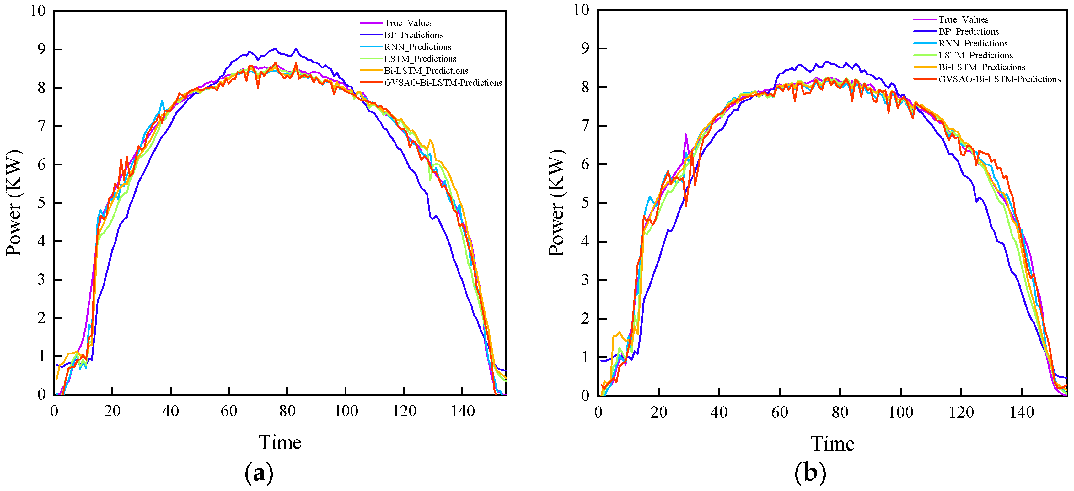
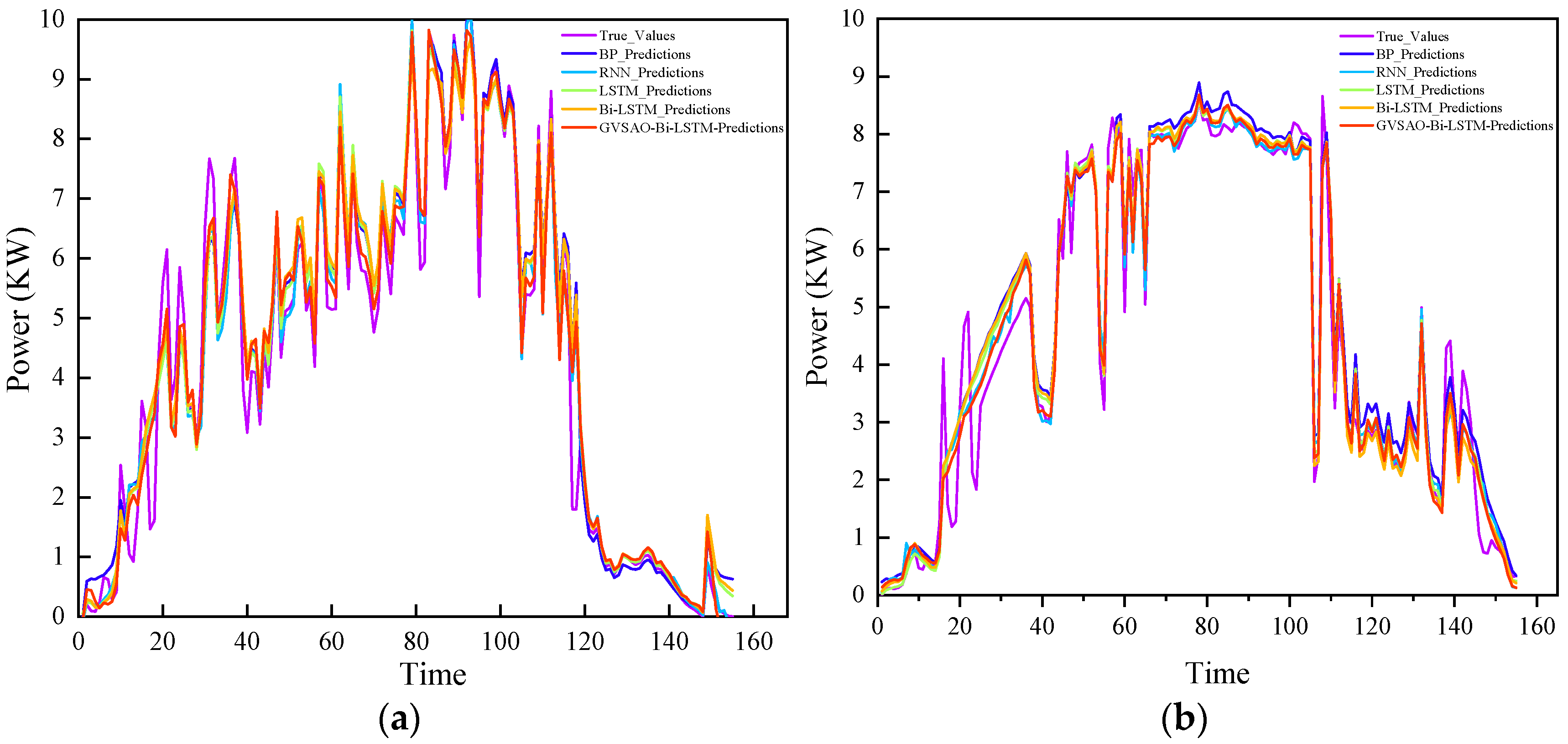
5.2. Case Verification and Analysis

In this study, the proposed method was implemented using the Python programming language, and a Bi-LSTM model was constructed based on the PyTorch deep-learning framework. The model training process utilized high-performance computing resources, including a computing cluster equipped with the NVIDIA RTX 4080 GPU, which provided exceptional capabilities for large scale data processing and complex model training. This section primarily outlines the procedures for data normalization and inverse normalization, as well as presenting the prediction results and error analysis under various weather conditions for PV power generation. These findings serve to validate the advanced and precise characteristics of the model.

(1)

Data normalization and denormalization procedures

$$X^{\prime }={\displaystyle \frac{X-X_{\min }}{X_{\max }-X_{\min }}}$$

(21)

Data normalization is a crucial step in the processing and analysis of data, particularly in the identification of analogous days and construction of predictive models. It facilitates comparison and computation of data with varying scales on a standardized scale. In this study, we employ the widely utilized min-max normalization method, which rescales the data to fit within the range of 0 to 1, thereby mitigating issues related to data overflow or numerical instability during training.

The process of denormalization involves restoring the data from its normalized range to its original range after normalization. The primary advantage of denormalization lies in its ability to restore the data to its original range, thereby enhancing the intuitive accuracy of predicting actual PV power generation. This process confers practical significance upon predicted results, facilitating convenient comparison between predicted and real data and thus enabling more effective evaluation of the model’s performance. The formula for inverse normalization is as follows:

$$X_{orig}=X_{norm}\times \left(X_{\max }-X_{\min }\right)+X_{\min }$$

(22)

where $X_{norm}$ represents the normalized data value, $X_{orig}$ denotes the original data value,$X_{\min }$ stands for the minimum value of the dataset, and $X_{\max }$ signifies the maximum value of the dataset.

(2)

Analysis of the prediction outcomes of PV power generation

For the K-means clustering analysis, weather is categorized into three groups: sunny, cloudy, and rainy. Five prediction models—BP neural network, RNN recurrent neural network, LSTM, Bi-LSTM, and GVSAO-Bi-LSTM—are established with consistent parameters to validate the effectiveness of the proposed model. Simultaneously, two days of each weather type are randomly selected for visual analysis as depicted in Figure 11, Figure 12 and Figure 13. The X-axis represents the time sequence starting from when the actual PV power generation exceeds 0 until it reaches 0 within a day; data is collected at 5-min intervals with a total of 156 data points per day. The Y-axis represents the actual value of PV power generation. During data preprocessing, normalization is performed to ensure comparability and calculation on a uniform scale across different datasets in order to enhance model stability and accuracy. In presenting results, inverse normalization is applied to the data; thus, the Y-axis reflects inversely normalized actual values of PV power generation.

As depicted in Figure 11, the PV power output exhibits remarkable stability under clear weather conditions, characterized by minimal fluctuations in solar irradiance. In the presence of stable irradiance conditions, various models demonstrate a high degree of fitting with actual measured values, exhibiting negligible errors and consistent performance. The predictable nature of solar panel output holds significant implications for the formulation of scheduling plans by the power dispatching department.

As depicted in Figure 12, the solar irradiance exhibits significant fluctuations under cloudy skies due to cloud obstruction, resulting in a more pronounced variation in the power curve of PV generation. In such complex weather conditions, the predictive challenges for each model are heightened; however, the enhanced model can still uphold high prediction accuracy. In practical applications, the dispatching department can devise appropriate scheduling plans based on these predictions to ensure power supply stability.

As depicted in Figure 13, the power curve of photovoltaic generation exhibits significant fluctuations during rainy conditions due to the influence of factors such as irradiation, temperature, and humidity. The unstable and low irradiation results in reduced actual photovoltaic generation power and a substantial deviation from the predicted value. Despite adverse weather conditions, the optimized model demonstrates remarkable robustness and adaptability. Ensuring accurate prediction of photovoltaic generation power under challenging weather conditions can effectively enhance system reliability and overall performance.

A box plot is a statistical graphic used to visually represent the distribution of a dataset, encompassing key statistics such as maximum, minimum, median, and other quartiles. Box plots offer an efficient and intuitive means to illustrate the central tendency and spread of data, as well as the symmetry and skewness of the distribution. They effectively convey the median and range of each dataset when comparing multiple datasets, providing a clear demonstration of their respective strengths and weaknesses. As depicted in Figure 14, Figure 15 and Figure 16, error box plots for prediction results under three distinct weather conditions are presented. The GVSAO-Bi-LSTM model exhibits the narrowest prediction error range across all weather conditions with a median close to 0. A comparison among the box plots reveals that all prediction models adeptly capture feature variations under relatively stable lighting conditions with minimal error ranges signifying significant predictive performance. Conversely, in more volatile lighting scenarios such as cloudy or rainy weather conditions, larger error ranges indicate limited predictive capabilities for each model. Nevertheless, relative to traditional models, the enhanced model demonstrates superior robustness and adaptability.

To assess the accuracy of the predictive model, this study utilizes a range of statistical indicators, including mean square Error (MSE), root mean square error (RMSE), mean absolute error (MAE), and mean absolute percentage error (MAPE). Among these, MSE provides an overall measure of predictive accuracy by squaring the prediction error and calculating the average; RMSE normalizes the value to the original data scale for enhanced interpretability; MAE quantifies the average predictive error by taking the absolute difference between predicted and actual values and averaging them, offering comprehensive insight into model performance; and MAPE evaluates relative prediction errors as a percentage, providing an intuitive measurement. The formulas for these indicators are provided below.

$$RMSE=\sqrt{{\displaystyle \frac{1}{n}}{\displaystyle \sum _{i=1}^n{\left(y_i-\widehat{y_i}\right)}^2}}$$

(23)

$$MAE={\displaystyle \frac{1}{n}}{\displaystyle \sum _{i=1}^n\left|y_i-\widehat{y_i}\right|}$$

(24)

$$MSE={\displaystyle \frac{1}{n}}{{\displaystyle \sum _{i=1}^n\left(y_i-\widehat{y_i}\right)}}^2$$

(25)

$$MAPE={\displaystyle \frac{100}{n}}{\displaystyle \sum _{i=1}^n\left|\frac{y_i-\widehat{y_i}}{\widehat{y_i}}\right|}\times 100\%$$

(26)

As shown in

Table 3. Comparison of model prediction error indexes under different weather conditions.

Weather Type	Model	Error Index
		MSE	RMSE	MAE	MAPE
Clear	BP	0.4462	0.6681	0.4813	95.81%
	RNN	0.3169	0.5629	0.3677	78.01%
	LSTM	0.2868	0.5356	0.3395	61.06%
	Bi-LSTM	0.2322	0.4819	0.2876	36.59%
	GVSAO-Bi-LSTM	0.2048	0.4526	0.2714	4.75%
Cloudy	BP	0.4529	0.6731	0.5152	335.20%
	RNN	0.3384	0.5817	0.3723	147.58%
	LSTM	0.2879	0.5366	0.3449	73.16%
	Bi-LSTM	0.2392	0.4891	0.3073	48.93%
	GVSAO-Bi-LSTM	0.2092	0.4574	0.2919	5.41%
Rainy	BP	0.5607	0.7489	0.5658	338.24%
	RNN	0.3549	0.5957	0.3774	259.27%
	LSTM	0.3517	0.5931	0.3711	141.08%
	Bi-LSTM	0.2898	0.5383	0.3338	73.32%
	GVSAO-Bi-LSTM	0.2714	0.5209	0.3241	14.37%

, the predictive performance is conspicuously robust under clear day conditions. Compared with conventional BP, RNN, LSTM, and Bi-LSTM models, the model investigated in this study presents reductions in MSE values by 0.2414, 0.1121, 0.082, and 0.0274, respectively. The corresponding decreases in MAPE values are 81.06%, 63.26%, 46.31%, and 21.84%.

Under cloudy day conditions, the predictive performance shows a slight decline. Nevertheless, the model under investigation in this study still reveals superiority over conventional models. Specifically, the MSE values of traditional BP, RNN, LSTM, and Bi-LSTM models are lowered by 0.2437, 0.1292, 0.0787, and 0.03, respectively. Furthermore, the MAPE decreased by 319.79%, 132.17%, 57.75%, and 33.52% for these respective models.

The predictive performance is significantly undermined in rainy conditions, as evidenced by the respective reductions in MSE values of 0.2893, 0.0835, 0.0803, and 0.0184 for the traditional BP, RNN, LSTM, and Bi-LSTM models, along with corresponding drops in MAPE values of 303.87%, 224.9%, 106.71%, and 38.95%, respectively. The findings reveal that the predictive potency of the model proposed in this paper possesses considerable superiority.

6. Conclusions

This study proposed an improved snow ablation optimization algorithm to optimize the Bi-LSTM network. By applying the optimal point strategy and periodic oscillation strategy, the key structural parameters of Bi-LSTM, such as the feature dimension at each time step and the number of LSTM hidden units in each layer, were optimized. The GVSAO-Bi-LSTM prediction model was constructed, which was used for predicting PV power generation. The research results show that the model has high accuracy in predicting PV power generation under sunny, cloudy, and rainy weather conditions. Compared with other methods, the GVSAO-Bi-LSTM model has significant advantages. This indicates that the method has high application value in improving the stability of PV power generation and power prediction accuracy.

References

1. Das, U.K.; Tey, K.S.; Seyedmahmoudian, M.; Mekhilef, S.; Idris, M.Y.I.; Deventer, W.Y.; Horan, B.; Stojcevski, A. Forecasting of photovoltaic power generation and model optimization: A review. Renew. Sustain. Energy Rev. 2018, 81, 912–928. [Google Scholar] [CrossRef]
2. Qiu, T.; Wang, L.; Lu, Y.; Zhang, M.; Qin, W.; Wang, S.; Wang, L. Potential assessment of photovoltaic power generation in China. Renew. Sustain. Energy Rev. 2022, 154, 111900. [Google Scholar] [CrossRef]
3. Hosenuzzaman, M.; Rahim, N.A.; Selvaraj, J.; Hasanuzzaman, M.; Malek, A.B.M.A.; Nahar, A. Global prospects, progress, policies, and environmental impact of solar photovoltaic power generation. Renew. Sustain. Energy Rev. 2015, 41, 284–297. [Google Scholar] [CrossRef]
4. Fu, X.; Zhang, C.; Xu, Y.; Zhang, Y.; Sun, H. Statistical Machine Learning for Power Flow Analysis Considering the Influence of Weather Factors on Photovoltaic Power Generation. IEEE Trans. Neural Netw. Learn. Syst. 2024, 109, 38587954. [Google Scholar] [CrossRef]
5. Amole, A.O.; Oladipo, S.; Olabode, O.E.; Makinde, K.A.; Gbadega, P. Analysis of grid/solar photovoltaic power generation for improved village energy supply: A case of Ikose in Oyo State Nigeria. Renew. Energy Focus 2023, 44, 186–211. [Google Scholar] [CrossRef]
6. Wang, X.; He, X.; Sun, X.; Qin, M.; Pan, R.; Yang, Y. The diffusion path of distributed photovoltaic power generation technology driven by individual behavior. Energy Rep. 2024, 11, 651–658. [Google Scholar]
7. Al-Duais, F.; Al-Sharpi, R. A unique Markov chain Monte Carlo method for forecasting wind power utilizing time series model. Alex. Eng. J. 2023, 74, 51–63. [Google Scholar] [CrossRef]
8. Zhou, B.; Chen, X.; Li, G.; Gu, P.; Huang, J.; Yang, B. Xgboost–sfs and double nested stacking ensemble model for photovoltaic power forecasting under variable weather conditions. Sustainability 2023, 15, 13146. [Google Scholar] [CrossRef]
9. Bai, R.; Shi, Y.; Yue, M.; Du, X. Hybrid model based on K-means++ algorithm, optimal similar day approach, and long short-term memory neural network for short-term photovoltaic power prediction. Glob. Energy Interconnect. 2023, 6, 184–196. [Google Scholar] [CrossRef]
10. Houran, M.A.; Salman Bukhari, S.M.; Zafar, M.H.; Mansoor, M.; Chen, W. COA-CNN-LSTM: Coati optimization algorithm-based hybrid deep learning model for PV/wind power forecasting in smart grid applications. Appl. Energy 2023, 349, 121638. [Google Scholar] [CrossRef]
11. Guo, W.; Xu, L.; Wang, T.; Zhao, D.; Tang, X. Photovoltaic Power Prediction Based on Hybrid Deep Learning Networks and Meteorological Data. Sensors 2024, 24, 1593. [Google Scholar] [CrossRef]
12. Li, C.; Pan, P.; Yang, W. Power Forecasting for Photovoltaic Microgrid Based on MultiScale CNN-LSTM Network Models. Energies 2024, 17, 3877. [Google Scholar] [CrossRef]
13. Liu, L.; Liu, D.; Sun, Q.; Li, H.; Wennersten, R. Forecasting power output of photovoltaic system using a BP network method. Energy Procedia 2017, 142, 780–786. [Google Scholar] [CrossRef]
14. Castillo-Rojas, W.; Bekios-Calfa, J.; Hernández, C. Daily prediction model of photovoltaic power generation using a hybrid architecture of recurrent neural networks and shallow neural networks. Int. J. Photoenergy 2023, 1, 2592405. [Google Scholar] [CrossRef]
15. Wang, L.; Mao, M.; Xie, J.; Liao, Z.; Zhang, H.; Li, H. Accurate solar PV power prediction interval method based on frequency-domain decomposition and LSTM model. Energy 2023, 262, 125592. [Google Scholar] [CrossRef]
16. Fan, Y.; Ma, Z.; Tang, W.; Xu, P. Using Crested Porcupine Optimizer Algorithm and CNN-LSTM-Attention Model Combined with Deep Learning Methods to Enhance Short-Term Power Forecasting in PV Generation. Energies 2024, 17, 3435. [Google Scholar] [CrossRef]
17. Zhang, J.; Hong, L.; Ibrahim, S.; He, Y. Short-term prediction of behind-the-meter PV power based on attention-LSTM and transfer learning. IET Renew. Power Gener. 2024, 18, 321–330. [Google Scholar] [CrossRef]
18. Wentz, V.H.; Maciel, J.N.; Ledesma, J.J.G. Solar Irradiance Forecasting to Short-Term PV Power: Accuracy Comparison of ANN and LSTM Models. Energies 2022, 15, 2457. [Google Scholar] [CrossRef]
19. Xiao, Z.; Huang, X.; Liu, J.; Li, C.; Tai, Y. A novel method based on time series ensemble model for hourly photovoltaic power prediction. Energy 2023, 276, 127542. [Google Scholar] [CrossRef]
20. Hu, Z.; Gao, Y.; Ji, S.; Mae, M.; Imaizumi, T. Improved multistep ahead photovoltaic power prediction model based on LSTM and self-attention with weather forecast data. Appl. Energy 2024, 359, 122709. [Google Scholar] [CrossRef]
21. Li, M.; Wang, W.; He, Y.; Wang, Q. Deep learning model for short-term photovoltaic power forecasting based on variational mode decomposition and similar day clustering. Comput. Electr. Eng. 2024, 40, 39–50. [Google Scholar] [CrossRef]
22. Lu, X.; Guan, Y.; Liu, J.; Yang, W.; Sun, J.; Dai, J. Research on Real-Time Prediction Method of Photovoltaic Power Time Series Utilizing Improved Grey Wolf Optimization and Long Short-Term Memory Neural Network. Processes 2024, 12, 1578. [Google Scholar] [CrossRef]
23. Chen, Y.; Li, X.; Zhao, S. A Novel Photovoltaic Power Prediction Method Based on a Long Short-Term Memory Network Optimized by an Improved Sparrow Search Algorithm. Electronics 2024, 13, 993. [Google Scholar] [CrossRef]
24. Liang, L.; Su, T.; Gao, Y.; Qin, F.; Pan, M. FCDT-IWBOA-LSSVR: An innovative hybrid machine learning approach for efficient prediction of short-to-mid-term photovoltaic generation. J. Clean. Prod. 2023, 385, 135716. [Google Scholar] [CrossRef]
25. Hua, L.; Wang, Y. Application of Number Theory in Modern Analysis, 1st ed.; China Science Publishing & Media Ltd.: Beijing, China, 1978; pp. 1–99. [Google Scholar]
26. Deng, L.; Liu, S. Snow ablation optimizer: A novel metaheuristic technique for numerical optimization and engineering design. Expert Syst. Appl. 2023, 225, 120069. [Google Scholar] [CrossRef]
Figure 1. Pearson correlation coefficient analysis graph.
Energies 17 04434 g001
Figure 2. K-means analysis flow chart.
Energies 17 04434 g002
Figure 3. Snow ablation process diagram.
Energies 17 04434 g003
Figure 4. Bi-LSTM schematic diagram.
Energies 17 04434 g004
Figure 5. LSTM schematic diagram.
Energies 17 04434 g005
Figure 6. GVSAO Flowchart.
Energies 17 04434 g006
Figure 7. F1 function test results.
Energies 17 04434 g007
Figure 8. F2 function test results.
Energies 17 04434 g008
Figure 9. F3 function test results.
Energies 17 04434 g009
Figure 10. Model construction flow chart.
Energies 17 04434 g010
Figure 11. Comparison of prediction results on sunny days. (a) Photovoltaic power generation forecast for the first random sunny day; (b) Photovoltaic power generation forecast for the second random sunny day.
Energies 17 04434 g011
Figure 12. Comparison of prediction results on cloudy days. (a) Photovoltaic power generation forecast for the first random cloudy day; (b) Photovoltaic power generation forecast for the second random cloudy day.
Energies 17 04434 g012
Figure 13. Comparison of prediction results on rainy days. (a) Photovoltaic power generation forecast for the first random rainy day; (b) Photovoltaic power generation forecast for the second random rainy day.
Energies 17 04434 g013
Figure 14. Error box plot of sunny forecast results.
Energies 17 04434 g014
Figure 15. Error box plot of cloudy forecast results.
Energies 17 04434 g015
Figure 16. Error box plot of rainy forecast results.
Energies 17 04434 g016