Comparison of the Energy Efficiency of Fixed and Tracking Home Photovoltaic Systems in Northern Poland

Abstract

The relevance of the article’s results lies in presenting the actual energy yields of PV panels of various generations and types of installations. The aim of the article is to provide answers about the effective operation of three different photovoltaic systems: a stationary off-grid system operated for several years, a stationary on-grid system, and a system mounted on trackers. A stationary on-grid system was used as the reference system, taking its area and energy yield as the reference point. The assessment was made on the basis of energy and cost efficiency analysis using the comparative method. The obtained results were compared to the results of other PV systems whose parameters were obtained from literature analysis. The analysis showed significant differences in adapting them to different sunlight conditions. The results confirmed the validity of using fixed PV panels (Installation II) in the short term and the advantage of the PV panel tracking system (Installation III) in the long term. The results also confirm that Installation I, despite its eight years of operation time, shows a relatively small decrease in efficiency, which confirms the validity of the long-term operation of the PV installation.

1. Introduction

In accordance with Directive (EU) 2018/2001 of the European Union [1], which defines levels of renewable energy used in the European Union and sets the renewable energy target for 2030, extensive measures should be taken to effectively reduce greenhouse gas emissions, boost energy efficiency, and create a reliable system of RES, with the aim of enhancing the security of the energy supply by engaging in significant technological and regional development in various areas [2,3].

Based on the annual report [4] published by PSE S.A. (a Polish electricity transmission systems operator) regarding the structure of the installed capacity of the KSE (the Polish National Grid) on 31 December 2020, the installed electric capacity exceeded 50 GW. This number includes conventional sources (commercial thermal power stations based on fossil fuels constituting 74.55% of this output) as well as all kinds of renewable sources (wind farms, photovoltaic installations, hydro power plants, as well as power plants based on biomass and biogas—constituting 25.45%) [5,6,7].

The rapid development of the sector based on individual photovoltaic installations necessitated an update on the structure of the KSE on 11 November 2022 [8], revealing that Poland had an installed electric capacity exceeding 53.6 GW. This figure includes conventional sources: commercial thermal power plants based on fossil fuels, constituting 67% of this capacity, as well as various kinds of renewable sources (wind farms, photovoltaic installations, hydropower plants, power plants based on biomass and biogas, accounting for 33%). Of the renewable sources, wind energy accounted for 36.7%, water 4.7%, biomass 4.6%, biogas 1.3%, and photovoltaics 52.7%. RES achieved a 35.4% (20.9 GW) share in the power sector in just a very short time. Most likely, this was due to the approaching deadline facing Poland related to the fulfillment of international obligations [9].

Such a high level of growth was achieved thanks to comprehensive action involving technological development, comprehensive government support (increase in prosumer contracts and subsidies for installations), and sociological concerns (the international energy crisis resulting from the war in Ukraine, general trends, the specter of energy price hikes due to carbon dioxide emission charges for conventional energy).

Changes in the support programs available for photovoltaic systems will probably undermine investor interest in this sector. At the same time, the huge number of systems that have been installed will soon cause many operational problems. Most of the existing photovoltaic systems built in Poland are permanent installations on the roofs of buildings with better or worse horizontal adaptation to the sun (the average installation size is 10.1 kWp) [10].

The projected decline in investor interest in this sector means that the decision to build a new installation will require a more careful consideration of many criteria and re-liable research based on operational experience. Interest in photovoltaic installations in Poland has basically decreased for three reasons as follows:

• First of all, there was a change in the status of new owners of photovoltaic installations in Poland. They stopped being prosumers with a quantitative settlement and were treated as energy producers with a financial settlement. This solution is less favorable for investors.
• Secondly, over the last five years, according to data from PSE (Polish Energy Networks), there has been a fivefold increase in the power installed in PV installations. The microgeneration market has been saturated with simple PV installations. New but much more expensive solutions have appeared (Smart Home Systems, PV tracking systems), and difference in investment costs for their use is not economically justified, which is partially shown in our article in relation to PV tracking systems.
• Thirdly, there has been a significant increase in the technical and economic awareness of potential investors. This translates into greater caution when investing in PV technology that is not supported by reliable technical information about the technology used.

This publication presents a comparison of the energy efficiency of these systems, an assessment based on efficiency analysis, and a determination of the operational factors that affect this efficiency. This collated experience will assist in the decision-making process regarding whether to purchase and operate a microgeneration system based on photovoltaic panels.

The paper is organized as follows. In the introduction, we provide a short description of the crucial need to develop PV systems that increase the share of renewable energy in the overall balance of energy produced. The next chapter presents the specifications of the tested installations. In the third chapter, the authors present the results of the energy yields of the considered PV installations. The fourth chapter sums up the cost efficiency of the considered PV installations, and in the next chapter (5), the authors discuss the energy yields of the analyzed PV installations in comparison to other systems installed in various places around the world, the data for which were obtained from the literature. The last chapter contains the conclusions from the conducted research and analyses.

2. Specifications of the Tested Installations

Currently, the Internet is full of information on experiences resulting from the operation of various photovoltaic installations. More often than not, these are user reports from the periodic operation of these systems. Particular emphasis is placed on the amount of energy produced and the payback period, usually calculated using a simple economic analysis. This approach plays a marketing role but does not take into account many factors affecting the final outcome of the operated or planned investment.

The rapid development of photovoltaic systems used in home micropower generation systems provides the basis for a broader analysis examining the operation of various types of photovoltaic systems. In order to perform a specific operational analysis of various photovoltaic installations, three micro-installations with different parameters (installed power, construction, operation time, energy conversion system, etc.) were considered as follows:

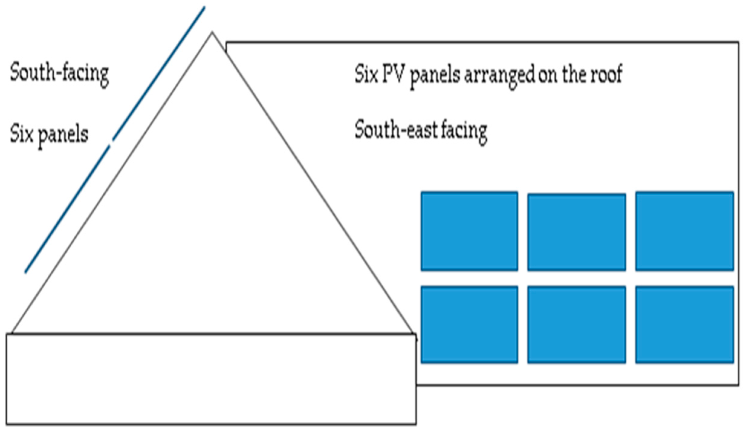
• Roof installed, off grid—year of construction 2014;
• Roof installed, on grid—year of construction 2020;
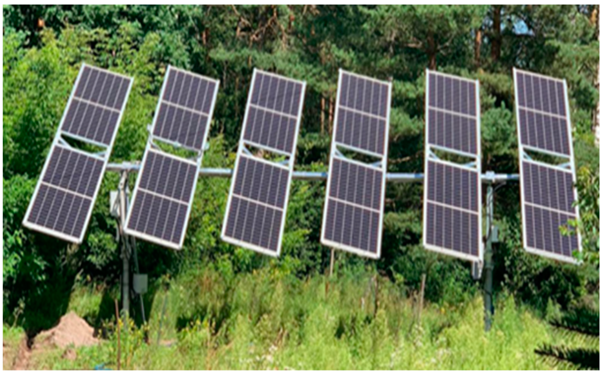
• Dual-axis tracking system, on grid—year of construction 2020.

Installation I—installed on the roof of the building in 2014 (Figure 1). The angle of inclination is 38° (detailed parameters in

Table 1. Basic technical and cost data of the tested installations.

		Installation I (2014) (Module Power 250W)			Installation II (2020) (Module Power 370W)			Installation III (2020) (Module Power 370W)
Name	IU	Quantity	Price per Item (USD)	Price (USD)	Quantity	Price per Item (USD)	Price (USD)	Quantity	Price per Item (USD)	Price (USD)
Photovoltaic module	pcs.	12	135.4	1625.3	14	149.2	2088.9	13	149.2	1939.7
Inverter	pcs.	1	270.9	270.9	1	1079	1079	1	1079	1079
Cables, supporting structure, and other elements	set	1	1489.8	1489.8	1	1607.2	1607.2	1	819.2	819.2
Dual-axis tracking system with motors	set	-	-	-	-	-	-	1	6366.8	6366.8

, Table 2 and Table 3). The system was designed as a stand-alone off-grid system using 100% of the generated electricity to power electric heaters in the heat exchanger. Currently (after expansion), the system consists of 12 panels with a power of 250 Wp (total power 3 kWp). The panels are arranged on two roofs facing 100° to the east and 190° to the south. This arrangement of panels results from the location of the building and the roof structure. Moreover, the panels are arranged so that they are shaded as little as possible. Unfortunately, this phenomenon occurs and is caused by elements of buildings (including neighboring buildings) and the adjacent forest. The system is not equipped with optimizers that turn off shaded panels but is divided into six circuits (strings) to limit this effect [11].

Installation II—standard, permanent, and installed on the roof of a building in 2020 (Figure 2). The angle of inclination is 30°, and the 14 polycrystalline panels with a power of 370 Wp were installed (detail parameters are included in Table 1, Table 2 and Table 3). The total system power is approximately 5.2 kWp. The installation is connected to the grid (on grid) and works within a prosumer system.

Installation III—a two-axis tracking system that was installed in 2020 (Figure 3). Thirteen panels with a power of 370 Wp are placed on the stand. The total power of the system is 4.8 kWp (detail parameters are included in Table 1, Table 2 and Table 3). The structure of the tracking system consists of a linear actuator driven by a three-phase induction motor (90 W/0.4kV AC) and transmission. This solution means the panels can be rotated east–west by a maximum angle of 270°. In order to enable the panels to rotate up and down, the second tracking system axis is equipped with a linear actuator driven by a DC motor (90 W/24V DC) with two limit switches installed. This enables north–south rotation by a maximum angle of 80°. This is controlled in an open system using the astronomical calendar.

The considered PV installations in a standard version with a back-up system, in order to protect against voltage surges, were equipped on the DC and AC side with dedicated varistor voltage surge protection (e.g., AC class B ETITEC-B 275/25), in accordance with the provisions of ETITEC-B-PV.

Electric shock protection complies with the provisions of the PN-HD 60364-4-41:2017-09 standard [12], using appropriate insulating enclosures for electrical devices and insulation of cables and wires. In the event of damage, protection is ensured by a rapid shutdown of the power supply using the factory circuit breaker (K60N-B16-3).

In the event of a fire, the PV system is protected by disconnecting the PV modules using a switch disconnector (IS-25/3), which is located in the PV switchboard.

The installations are provided with lightning protection via earthing in accordance with the PN-EN 62305-4:2011 standard [13].

In order to carry out a comparative analysis of the basic technical and economic specifications, Table 1 contains the specifications of the photovoltaic modules. Table 2 presents some basic data concerning the discussed microgeneration installation and Table 3 contains the specifications of PV energy conversion modules installed in the tested installations.

Table 2. Basic specs of photovoltaic modules installed at the tested sites.

		Installation I3 kWp (2014)	Installation II5.2 kWp (2020)	Installation III4.8 kWp (2020)
Module type	(-)	MS250P-60	SV120M.3.2-370	SV120M.3.2-370
Max. power	Pmax (W)	250	370	370
Open-circuit voltage	Uoc (V)	37	40.9	40.9
Max. power voltage	Umpp (V)	26	34.3	34.3
Short-circuit current	Isc (A)	9.12	11.49	11.49
Max. power current	Imppt (A)	8.71	10.79	10.79
Efficiency	(%)	17.1	20.3	20.3
Insolation [14]	(kWh/m2)	1070	985	985
Temperature coefficient of Pmax	%/°C	−0.407	−0.36	−0.36

Table 2. Basic specs of photovoltaic modules installed at the tested sites.

		Installation I3 kWp (2014)	Installation II5.2 kWp (2020)	Installation III4.8 kWp (2020)
Module type	(-)	MS250P-60	SV120M.3.2-370	SV120M.3.2-370
Max. power	Pmax (W)	250	370	370
Open-circuit voltage	Uoc (V)	37	40.9	40.9
Max. power voltage	Umpp (V)	26	34.3	34.3
Short-circuit current	Isc (A)	9.12	11.49	11.49
Max. power current	Imppt (A)	8.71	10.79	10.79
Efficiency	(%)	17.1	20.3	20.3
Insolation [14]	(kWh/m2)	1070	985	985
Temperature coefficient of Pmax	%/°C	−0.407	−0.36	−0.36

Table 3. Basic specs of energy conversion modules installed at the tested sites.

		Installation I (2014)	Installation II (2020)	Installation III (2020)
Module type of inverter	(-)	Omega S1	FroniusSymo5.0-3-M	FroniusSymo5.0-3-M
Max. input current	(A)	7/15/24	16	16
Min. input current	Umin (V)	25	150	150
Nominal input voltage	Unom (V)	52	595	595
Max. input voltage	Umax (V)	90	1000	1000
MPPT voltage range	(V)	40–90	163–800	163–800
Max. output current	(A)	7/15/24	13.5	13.5
Range of adjustable output voltage	(V)	40–90	260–485	260–485
Frequency	(Hz)	-	50	50
Internal night power consumption	(W)	<1	<1	<1

Table 3. Basic specs of energy conversion modules installed at the tested sites.

		Installation I (2014)	Installation II (2020)	Installation III (2020)
Module type of inverter	(-)	Omega S1	FroniusSymo5.0-3-M	FroniusSymo5.0-3-M
Max. input current	(A)	7/15/24	16	16
Min. input current	Umin (V)	25	150	150
Nominal input voltage	Unom (V)	52	595	595
Max. input voltage	Umax (V)	90	1000	1000
MPPT voltage range	(V)	40–90	163–800	163–800
Max. output current	(A)	7/15/24	13.5	13.5
Range of adjustable output voltage	(V)	40–90	260–485	260–485
Frequency	(Hz)	-	50	50
Internal night power consumption	(W)	<1	<1	<1

The first of the discussed photovoltaic micro-installations was installed over nine years ago, which is why it represents a different technical level. These installations have different measurement and data recording systems. In installation No. 1, the following parameters are recorded: voltage, current, power, and electricity. These measurements are based on a system built into the MPPT (Maximum Power Point Tracking) voltage optimizing system and on the Circutor MK-30-DC universal measuring unit with the following technical specifications: voltage measurement up to 125 V DC ± 0.5% FS ± 1% digit, current measurement up to 30 A DC ± 0.5% FS ± 1% digit, and power measurement up to 4.5 kW DC ± 1% FS ± 1% digit. Measurements in Installations II and III are based on data collected from the Fronius photovoltaic inverter with the “solarweb” application. For comparative purposes, the results in the tables have been converted to the capacity of standard installation No. 2.

The phenomenon of shading occurs in the examined Installation I. This was taken into account in the description of Installation I, which talks about the division of the installation and work into two planes, eastern and southern. The western plane was not used precisely because of the phenomenon in question. The next two Installations (II and III) are free from this phenomenon. The authors relied on data on energy yield. Therefore, this phenomenon is included in the obtained measurement results. In order to make the presented results more representative, the obtained energy yields were presented as average values.

3. Energy Yields of the Considered PV Installations

The following comparative criteria were adopted to run a multi-faceted analysis of photovoltaic installations:

• Efficiency was understood as an energy source operating in a specific geographic and time period;
• Cost effectiveness was understood as an investment with a specific depreciation;
• Operation was understood as a technical object subject to wear and tear over time.

Table 4. Production of electricity from installation No. 1 during its operation.

No.	Year of Energy Production	Energy Produced (kWh)	Total Energy Produced (kWh)
1	2014	6.2	6.2
2	2015	2201	2207
3	2016	1798	4005
4	2017	2016	6021
5	2018	1849	7870
6	2019	1646	9516
7	2020	1832	11,348
8	2021	1728	13,076
9	2022	1569	14,645

and Figure 4 present a summary of annual electricity production yields from installation No. 1 during the years of its operation. The calculated R² coefficient is ~0.64, which means a low agreement of the theoretical trend line with the experimental data. This confirms the fact that there were large weather differences in the individual years of operation affecting energy yields.

Installation I was manufactured in 2013 and has been in service since 2014. In order to compare it with the younger installations considered here, its rated power was converted to that of Installation III, which was taken as the model. The conversion involved adopting the area factor of the tested installation, which determines the ratio of the area of the considered installation (Installations II and III) to the reference installation (Installations III and I for comparison with Installation II).

Table 5. Monthly energy conversion in the tested installations in the recorded time period (1 July 2020 to 31 December 2020).

Month	Installation I (2014)(kWh)	Installation II (2020)(kWh)	Installation III (2020)(kWh)
July	610.3	705.8	914.0
August	476.1	665.7	947.0
September	381.7	493.9	695.2
October	204.9	278.4	363.4
November	87.5	116.9	188.7
December	43.0	45.2	110.3
Total	1803.5	2305.9	3218.6

,

Table 6. Monthly energy conversion in the tested installations in the recorded time period (1 January 2021 to 31 December 2021).

Month	Installation I (2014) (kWh)	Installation II (2020) (kWh)	Installation III (2020) (kWh)
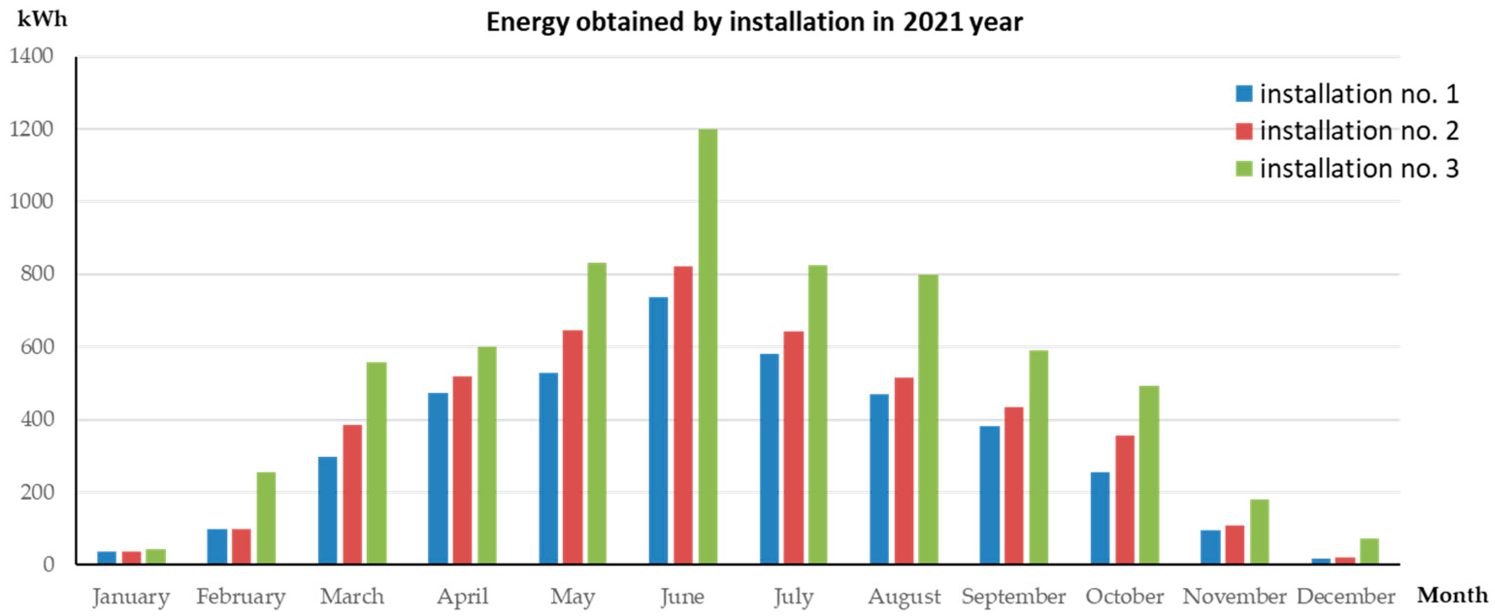
January	38.2	36.8	43.2
February	98.1	98.2	256.4
March	299.0	385.4	558.5
April	473.5	520.6	599.7
May	527.2	645.7	832.0
June	736.4	820.5	1199.7
July	582.4	643.4	826.3
August	469.1	517.1	799.6
September	381.7	434.8	591.8
October	255.8	357	491.4
November	95.5	108.4	180.9
December	18.0	20.9	72.3
Total	3974.9	4588.8	6451.8

and

Table 7. Monthly energy conversion in the tested installations in the recorded time period (1 January 2022 to 31 December 2022).

Month	Installation I (2014) (kWh)	Installation II (2020) (kWh)	Installation III (2020) (kWh)
January	42.8	23.9	86.6
February	148.0	88.4	474.3
March	464.3	412.6	501.5
April	472.1	448.9	581.8
May	471.7	554.9	878.3
June	497.7	813.1	1227.7
July	473.8	545.5	819.1
August	514.0	586.6	703.3
September	276.5	351.2	607.3
October	192.7	298.9	434.6
November	47.0	92.9	152.1
December	8.7	15.5	64.8
Total	3609.3	4232.4	6531.4

show the efficiency outcomes obtained for all installations at the same time.

The same time interval for recording the energy yield data (1 July 2020 to 31 December 2022) was used to compare the energy efficiency of the systems in question. The tests were carried out in similar climatic conditions (average monthly horizontal radiation = 2.76 kWh/m²).

The apparent decrease in this installation’s efficiency, calculated as a relative difference based on the value of the beginning and end of the trend line, is almost 29%. This difference in energy yield boils down to differences, inter alia, in the efficiencies of both installations (16.3%), which results from the technological progress of the considered installations and wear and tear resulting, for example, from matting of the surface, contamination with bird droppings, micro-cracks and corrosion of metallic connections, and changing weather conditions in the period under consideration. Installation I is inspected every year in the spring and the PV panel surfaces are washed. Periodical increases in the energy efficiency of the compared installations result mainly from insolation differences in individual locations (northern Poland) 50 or so kilometers apart. Graphical interpretation of the output of the discussed photovoltaic installations in 2021 is presented in Figure 5 and in 2022 is presented in Figure 6.

Table 7 and

Table 8. Comparison results of the tested installations.

Period of Operation	Comparison of Installations
	Installation I/II (%)	Installation III/II (%)	Installation III/I (%)
1 July–31 December 2020	−21.8	39.6	78.5
1 January–30 June 2021	−15.4	39.2	60.6
1 July–31 December 2021	−15.5	42.3	64.3
2021	−15.4	40.6	62.3
1 January–30 June 2022	−11.7	60.1	78.9
1 July–31 December 2022	−25	47.1	83.9
2022	−17.3	54.3	81

Note: In order to be able to compare it with Installations II and III, Installation I was converted to a comparable installed power of 4.8 kWp. Explanation: Installation I consists of two planes of panels placed east and south with a power of 3.08 kWp. This arrangement of panels and their mutual shading means that the actual power of the installation is 2.5 kWp—the measured value is 2 kWp. The converted energy value was obtained from the power ratio of Installations II, III, and I, 4.8 kWp/2.25 kWp, multiplied by the actual energy yield.

suggest the conclusion that the annual energy yields for individual installations differ, although the calculation area is assumed to be the same.

This is due to the arrangement of the surface of the PV panels relative to the sun. The first installation has two equal groups of panels, one facing east and the other facing south. In both cases, the angle of panel inclination is 35°. The analysis indicates that the annual yield may be influenced by weather conditions, so 2020 and 2022 were comparable years, while the energy yield in 2021 was 10% higher. The annual yield was obtained by multiplying the energy obtained during half a year of PV panel operation by two. Installation II has one group of panels facing south at an angle of 30°. The analysis shows that the energy yield in 2020 and 2021 was comparable, while in 2022 it was 8.4% lower. This difference between the yields of Installations I and II relates to the different weather conditions in which these installations operated, despite the relatively short distance between them. Installation III, which has one group of panels positioned to catch the maximum insolation potential due to its tracking system, presented the smallest annual changes, which do not exceed 1.2% for the analyzed period. It follows that over the study period, the two-way installation was the most sensitive to weather conditions due to the fact that only one part of the installation operates at a certain angle of insolation. Installation III with its tracking system is the least sensitive to years of better or worse weather.

The three installations differ in terms of efficiency. Installation I has an efficiency of 17%, while Installations II and III are based on modules of the same type and have an efficiency of 20.3%, which means that these installations are 16.3% more efficient than Installation I. The comparison presented in column 2 of Table 8, after taking into account the variance in efficiency, shows a similar difference in energy yield between Installations I and II. In this case, the difference in energy yields boils down solely to the difference in efficiency due to technological progress. The lack of remarkable differences is probably due to the short observation period during which the installations were compared. In such a short time (2.5 years), no differences were caused by wear and tear.

The third column of Table 8 contains a comparison of two installations made in the same panels with the same efficiency, thus referring to the yield related to the tracking system, which is not less than 39.2%; the maximum yield from the tracking installation is 60.1%, with an average of 46%.

A comparison of the yields of Installations III and I is presented in column 4 of Table 8. The energy yields of Installation III are significantly higher than those of Installation I and range from less than 61% to almost 84%. This difference includes the difference in the efficiency of both installations and operational wear and tear but mainly results from the use of a tracking system and optimization of the angle at which the sunlight hits the surface of the PV panels. A detailed specification of the dependencies of the individual components of the yield is not possible, as it would require additional data, such as a measurement of the intensity of sunlight for each installation. For research purposes, the use of devices that measure light intensity might be considered.

Based on the analysis of the data obtained, it can be said that the energy yield in a similar insolation environment is influenced by technical details and changes in the structure of the PV system resulting from operation.

4. Cost Efficiency of the Considered PV Installations

In order to analyze the cost effectiveness of the discussed installations, economic calculations were carried out using simple as well as more complex financial analysis formulas based on actual and estimated data. Actual data include energy yield during the operation of the installations, and estimates were adopted based on the analysis of the operating trends presented by these installations.

The discussed installations looked good and did not benefit from subsidies. In Installations II and III, the subsidy investment funds were taken into account in economic calculations in such a way that the initial investment cost was reduced by the funds obtained from the subsidy. The information obtained from investors concerned the actual investment costs incurred by the investor.

A typical SWOT analysis for each installation is presented in

Table 9. The SWOT analysis for each installation.

Strengths:	SWOT Installation I	Weaknesses:
Simple uncomplicated installation. Simple operational supervision. Consistent comparable (despite the time of) operation energy. Off-grid installation heating with a heat exchanger and cooperation with the UPS.		Potential for internal failures resulting from aging structural and electronic components subjected to environmental conditions.
Opportunities:		Threats:
Good weather gives higher energy yields. Operation during power outages.		Bad weather, rapid wear and tear of installations due to environmental impacts, and technological advances.
Strengths:	SWOT Installation II	Weaknesses:
Simple uncomplicated installation. Simple operational supervision. Consistent comparable (despite the time of) operation energy. On-grid installation and cooperation with the power grid.		Potential for internal failures resulting from aging structural and electronic components subjected to environmental conditions. No operation in the event of a power outage to the power grid.
Opportunities:		Threats:
Good weather gives higher energy yields.		Bad weather, rapid wear and tear of installations due to environmental impacts, and technological advances.
Strengths:	SWOT Installation III	Weaknesses:
Gain some electricity independence. On-grid installation and cooperation with the power grid.		Complicated installation requiring technical supervision. Potential for internal failures resulting from aging structural and electronic components subjected to environmental conditions. No operation in the event of a power outage to the power grid.
Opportunities:		Threats:
Good weather gives higher energy yields. Excellent energy matching.		Bad weather, rapid wear and tear of the installation resulting from environmental impacts, and technological advances.

.

The comparison of cost effectiveness was based on the direct return analytical method (simple rate of return on capital). This method determines the ratio of the annual profit to the amount of capital involved in a given investment project. The disadvantage of this method is that it is based on one-year values and does not take into account changes in the value of money over time [15].

RW = ZN/KW

(1)

where RW is the rate of return on equity, ZN is the annual net profit (USD), and KW is the amount of equity.

A more complex comparison of installation efficiency is based on the NPV (net present value) method, which can be used to assess relatively complex cash flows related to a project [16].

$$NPV={\sum }_{i=1}^n{\displaystyle \frac{C{F}_i}{{(1+r)}^n}}-J_0$$

(2)

where J₀ is the outlays; CF is the cash flows, n is the number of periods considered, and r is the rate of return.

Net present value is the sum of discounted cash flows, which are then reduced by the initial capital expenditure. The result of the analysis is read in such a way that if the NPV is ≥0 after the calculations, the investment is profitable. It may also indicate after which settlement period the result becomes positive. So, the depreciation period of the investment can be assessed.

The results are presented in

Table 10. Estimated financial flows from an assessment of the installations’ depreciation.

Year (Years)	Current and Estimated Price per 1 kWh (USD)	Installation I (2014)				Installation II (2020)				Installation III (2020)
		Current and Estimated Energy Production (kWh)	Financial Gain (USD)	Financial Flow (USD)	Discounted Cash Flow NPV (USD)	Current and Estimated Energy Production (kWh)	Financial Gain (USD)	Financial Flow (USD)	Discounted Cash Flow NPV (USD)	Current and Estimated Energy Production (kWh)	Financial Gain (USD)	Financial Flow (USD)	Discounted Cash Flow NPV (USD)	Desired Installation Cost (USD)
0	Investment cost >			−3578.4	−3578.4	Investment cost >		−6419.5	−6419.5	Investment cost >		−13,456.6	−13,456.6	−9456.6
1	0.152	2201	335.2	−3243.2	−3265.2	3670	558.9	−5860.7	−5887.3	5162	786.1	−12,670.4	−12,708	−8709.3
2	0.159	1798	286.1	−2957.3	−3010.7	3386	538.6	−5322	−5398.6	5229	831.8	−11,838.6	−11,953.4	−7955.2
3	0.167	2016	336.8	−2620.4	−2721.4	3489	583	−4739.1	−4895.2	5138	858.2	−10,980.4	−11,212	−7214.0
4	0.175	1849	324.1	−2296.4	−2456.8	3451	604.8	−4134.5	−4397.7	5081	890.4	−10,090	−10,479.5	−6482.5
5	0.182	1646	299.3	−1997.3	−2223.4	3413	620.4	−3513.9	−3911.6	5025	913.6	−9176.4	−9763.6	−5765.9
6	0.191	1832	349.8	−1647.5	−1962.5	3375	644.3	−2869.5	−3430.7	1129.5	948.9	−8227.5	−9055.4	−5057.8
7	0.200	1728	346.4	−1301.1	−1719.5	3338	669.1	−2200.4	−2955.2	4915	985.2	−7242	−8355.2	−4359.2
8	0.210	1569	330.2	−970.9	−1478.2	3301	694.8	−1505.7	−2485	4861	1023.2	−6219.1	−7662.7	−3668.3
9	0.221	1809	399.5	−571.1	−1220.7	3265	721.4	−784.3	−2020	4808	1062	−5156.8	−6978.2	−2983.4
10	0.232	1789	414.8	−156.6	−966.1	3229	748.6	−35.7	−1560.4	4755	1102.3	−4054.5	−6301.4	−2306.1
11	0.243	1769	430.2	273.6	−714.5	3194	776.6	740.9	−1106.4	4703	1143.6	−2910.9	−5632.7	−1637.9
12	0.254	1750	445.4	719.1	−466.6	3159	804.1	1545	−658.6	4651	1183.9	−1727	−4973.6	−980.1
13	0.267	1730	462.3	1181.6	−221.4	3124	835	2379.8	−215.9	4600	1229.3	−497.7	−4321.6	−328.8
14	0.280	1711	479.8	1661.4	21.1	3089	866.4	3246.4	221.8	4549	1275.9	778.2	−3677.3	314.5
15	0.294	1693	498.2	2159.8	260.7	3055	899.3	4145.7	654.3	4499	1324.1	2102.5	−3040.2	950.8
16	0.309	1674	517	2676.6	497.7	3022	933.4	5078.9	1082	4450	1374.3	3476.8	−2410.7	1580.7
17	0.324	1656	536.6	3213.4	731.8	2989	968.6	6047.5	1504.5	4401	1426.4	4902.9	−1788.4	2202.8
18	0.340	1637	557	3770.4	963.2	2956	1005.7	7053.2	1922.5	4352	1480.9	6383.9	−1173	2817.7
19	0.357	1619	558	4348.4	1192	2923	1043.6	8096.8	2335.4	4304	1536.8	7920.7	−564.8	3425.7
20	0.375	1601	600	4948.4	1418.2	2891	1083.4	9180.4	2743.9	4257	1595.4	9516.1	36.6	4027.4
21	0.393	1585	623.6	5572	1641.8	2859	1124.8	10,305.2	3147.5	4210	1656.4	11,172.5	631.1	4621.3
22	0.413	1567	647	6219.1	1863.2	2828	1167.7	11,473	3546.8	4164	1719.5	12,892	1218.9	5209.2
23	0.433	1549	671.4	6890.4	2081.6	2797	1212	12,685.2	3941.4	4118	1784.8	14,677	1800	5789.7
24	0.454	1532	696.4	7586.8	2297.7	2766	1257.3	13,942.5	4331.4	4073	1851.4	16,528.2	2374	6363.0
25	0.477	1516	723.6	8310.2	2511.4	2736	1305.7	15,248	4716.8	4028	1922.5	18,450.7	2941.8	6930.4

Note: Red indicates the excess of investment costs over the profit obtained from the installation.

. The following assumptions were made for calculations using the NPV method:

• The total (taking into account all elements) average price for electricity in the years 2014–2020 was—USD 0.15/kWh. Due to the abrupt increase in energy prices in 2023, a 5% linear annual increase in energy prices was assumed.
• Decrease in electricity production efficiency resulting from operational processes: 1.1%/year.
• Investment cost in year zero of individual photovoltaic installations: No. 1: USD 3578.5; No. 2: USD 6419.5; and No. 3: USD 13,456.6.
• The estimated, averaged annual electricity production of each tested photovoltaic installation, determined on the basis of measurements, is as follows: No. 1—1850 kWh; No. 2—3500 kWh; and No. 3—5200 kWh.
• Billing system for calculating profit for Installation II: 100% of the energy yield was used in the off-grid system. Installations II and III: an 80% on-grid prosumer system (80% user, 20% energy supplier for storage).
• The number of annual calculation periods is n = 25.
• The assumed rate of return based on the interest rate on long-term treasury bonds—CAGR (cumulative annual growth rate) [17,18]. For Installation I is used data for the first 8 years real exploatation, and for the other installations used forecast data with an r average (r average 5%). Note: If energy prices in a given country increase by more than the assumed 5%, the investment amortization time will shorten proportionally.
• The last column of Table 10 presents a simulation of the desired cost of the top-up installation, which will pay off at the same time as installations No. 1 and No. 2.

Based on the analysis of the data presented in Table 10, the following are determined:

• Installation I financial flow: 10 years; discounted cash flow NPV: 13 years;
• Installation II financial flow: 10 years; discounted cash flow NPV: 13 years;
• Installation III financial flow: 13 years; discounted cash flow NPV: 19 years;
• Installation III financial flow: simulation of the desired cost of the tracking PV installation; discounted cash flow NPV: 13 years.

Based on the analysis of the data presented in Table 10, it can be concluded that currently, the fixed photovoltaic Installation II achieves the fastest rate of financial return. Even though Installations I and II have the same financial payback periods, it is necessary to take into account the fact that Installation II provides a larger amount of energy at the same time, and at the end of the analysis period (after 25 years), the profit from Installation II is almost twice the NPV profit from Installation I. Although Installation III provides the largest amount of energy, its investment cost makes it unprofitable, and at the end of the analysis period (after 25 years), the NPV profit from Installation II exceeds the profit from Installation III by almost 1.6 times. However, when it comes to financial flow, the highest return at the end of the analysis period is achieved by Installation III. It follows that the cost of building an installation with a tracking system is decisive in this analysis.

Taking into account the assumption of the highest energy yield, the authors calculated the desired investment cost of Installation III. The cost of this installation should be USD 4000 lower than currently and USD 3000 higher than Installation II—this is the cost of constructing the PV tracking system installation structure along with the control module. Then, the return on investment will be comparable to stationary installations. At the same time, in the considered 25-year operating period, Installation III will achieve the highest profit. Striving to optimize (reduce) the costs of implementing a PV tracking system installation is an action aimed at popularizing this type of solution, thus achieving greater profit from the same area of PV panels. It seems that the cost of implementing the PV tracking system installations will decrease as the number of their implementations increases, cheaper solutions are developed, and competition increases, but at the moment, it is difficult to estimate this level. It will probably reach a level between the desired installation cost shown in Table 10 and the current cost of implementing the PV tracking system installation.

The literature [19,20,21] additionally mentions that the following actions affect the cost-effectiveness of photovoltaic systems and are associated with additional costs. These include servicing, leasing, and maintaining the site and insuring the installation, security, and possible taxes.

Although photovoltaic installations, due to their rapid development, are subject to a very fast process of technological aging, the analysis showed that the operation of the oldest installation (No. 1) is still economically viable. This process may result in the need to change the technology before depreciation sets in—e.g., as a result of the lack of spare parts for installations installed several years ago. Nevertheless, as long as the installation is operational, it should be used as long as possible because the difference in yield mainly stems from the percentage change in efficiency.

5. Discussion

An overview of comparisons between fixed and tracking PV systems obtained from the literature analysis is presented in

Table 11. The comparison of chosen fixed and tracking PV installations.

No	Title of the Article	Energy (MWh)		Difference (%), Localization
		Fixed	Tracker
1.	This article: Comparison of the Energy Efficiency of Fixed and Tracking Home Photovoltaic Systems in Northern Poland	4.45	6.48	2.5 years of measurement for Installations I and II and >8 years for Installation I: from 39.2 to 60.1 (average 46) Poland: Installation I 54.6° N, Installations II and III 53.8° N
2.	Energy efficiency analysis of 1 MW PV farm mounted on fixed and tracking systems [22]	1080	1293	16.5 Kuyavian-Pomeranian Voivodeship, Poland, latitude 53° N
3.	Environmental life cycle analysis of a fixed PV energy system and a two-axis sun tracking PV Energy system in a low-energy house in Turkey [23]	1.34	2.13	Only July (max): 35.1, July–December: 31 Sakarya, Turkiye, latitude 41° N
4.	Performance comparison of a double-axis sun tracking versus fixed PV system [24]	11.53	15.98	30.8, Muğla, Turkiye, latitude 37° N
5.	Design and Simulation of a Solar Tracking System for PV [25]	-	-	From 22 to 56 Northern Algeria, latitude 36° N
6.	Impact of PV System Tracking on Energy Production and Climate Change [26]	1710	2171 2234	21.2 fixed vs. one axis 23.5 fixed vs. dual axis 2.8 one axis vs. dual axis Townsville, Australia, latitude 19° S
7.	Innovative sensorless dual-axis solar tracking system using particle filter [27]	0.017	0.02	60 days: average 20.1, max. 38.5 Bangkok, Thailand, latitude 12.8° N
8.	Comparison of Energy Production Between Fixed-Mount and Tracking Systems of Solar PV Systems in Jakarta, Indonesia [28]	1.38	1.67	15–29, average 21, Jakarta, Indonesia, latitude 6° S
9.	Comparative performance analysis between static solar panels and single-axis tracking system on a hot climate region near to the equator [29]	0.00117	0.00131	13–20 July 2014: 11.5, one-axis PV Mossoro, Brazil, latitude 5.2° S
10.	Performance Comparison between Fixed and Dual-Axis Sun-Tracking Photovoltaic Panels with an IoT Monitoring System in the Coastal Region of Ecuador [24]	0.04	0.047	21 days: 19.6, Manabí, Ecuador, latitude 1° S
11.	Improvements of photovoltaic systems by using solar tracking in equatorial regions [30]	1.9	2.5	27.3 fixed vs. one axis 31 fixed vs. dual axis max. 6.5 average for one axis vs. dual axis Quito, Ecuador, latitude 0.2° S

, which shows a comparison of fixed and tracking PV systems deployed in various locations around the world.

The first row in Table 1 was completed based on the installation tests carried out in this article.

The issue of improving the efficiency of photovoltaic systems through the use of tracking systems is becoming more and more common around the world. The criterion for assessing their performance is presented in different ways. The dominant evaluation criterion is based on energy yield (presented in any way adopted by the authors of the analysis, e.g., quantitative, percentage), but there is also a comparison of instantaneous power, investment, and operating costs, as well as a percentage increase in power and a reduction in CO₂ emissions or investment payback time. Research on the energy efficiency of these systems is multi-track, e.g., systems already constructed and operating in various geographical and hydrometeorological conditions are analyzed, and the research includes the design and testing of new solutions adapted to specific conditions. Table 1 presents an overview of various solutions for photovoltaic installations and their energy yields mounted on tracking systems compared to systems with a fixed position in relation to the ground. The above comparison is arranged by latitude from high latitudes to the equator. Analysis of the compiled articles showed that the testing times described vary, from short trials lasting a few days to long-term trials spanning several years, such as those described in the article. Below is a brief discussion of each of the articles analyzed. Articles 2, 3, 8, and 12 contain analyses of energy yields between different types of systems (stationary, single-axis, and dual-axis trackers) based on computer simulations. Articles 3, 4, 5, 7, 9, and 10 contain analyses of energy yields based on tests of real PV installations. Article 3 contains a hybrid comparison and a simulation and test, and Article 6 analyzes survey data.

5.1. Article 2: Energy Efficiency Analysis of 1 MW PV Farm Mounted on Fixed and Tracking Systems

The article presents a comparison of the results of the simulation of electricity production of a photovoltaic farm installation with a sun-tracking system and a stationary farm. The comparison was carried out using the computer program PVSyst. The simulations were carried out in the same weather conditions for farms with identical capacities (1014 kWp) constructed based on identical panels with a unit power of 500 Wp. The obtained comparative results are the result of calculations based on the assumed data on the amount of solar energy falling on the area where the farm is installed (Kujawsko-Pomorskie Voivodeship in Poland) in a specific time obtained from the literature. The authors prove a 20% energy advantage of the tracking systems. At the same time, they explain that these investments are not very profitable due to the high investment costs. However, they see additional benefits of tracking systems, distinguishing the facilitation of operation of such systems in the form of easy access, the possibility of forced panel positioning, etc.

5.2. Article 3: Environmental Life Cycle Analysis of a Fixed PV Energy System and a Two-Axis Sun Tracking PV Energy System in a Low-Energy House in Turkey

The authors, based on experience gained from testing 80 W photovoltaic systems in a stationary and tracking configuration and on solar radiation data, proposed a project for powering a single-family home in Sakarya, Turkey. Based on the estimated average energy load of the receivers in the home, the size of the necessary stationary photovoltaic source (7 × 250 W panels) and tracking photovoltaic source (5 × 250 W panels) was estimated. Based on experience gained from the test systems and theoretical calculations, the energy efficiency of the individual solution and the depreciation of the individual solutions were determined. Based on the analysis of the information contained in the article, the authors determined a 35% increase in the obtained energy of the tracking system compared to the stationary system (energy yield per year 1.34 to 2.13 MWh). At the same time, matching the size of the tracking system to the required energy supply conditions of the home allows for better depreciation results for the tracking system than for the stationary system (11.9 years to 15.3 years).

5.3. Article 4: Performance Comparison of a Double-Axis Sun Tracking Versus Fixed PV System

The paper presents the results of the performance tests during one year of operation of two dual-axis tracking photovoltaic systems with a power of 7.9 KWp installed on the campus of Mugla University. The experiment was carried out in two stages. In the first case, the systems were locked in a fixed specified position, and then in the second case, the tracking systems were released. Thus, the same objects but two different configurations were subjected to comparative analysis. Moreover, the obtained experimental results were compared with the theoretical calculations of the energy yield from these installations. Based on the tests, almost 31% energy yield from the tracking systems was found (11.53 MWh to 15.98 MWh) and a 5% error between the simulated and measured values of the energy yield from the tested installations was determined.

5.4. Article 5: Design and Simulation of a Solar Tracking System for PV

The paper reports on the implementation of a new idea consisting of the development of an automatic microcontroller, whose task is to track the sun in an optimal way using hybrid, sensory, and chronological control algorithms. The implementation of this idea aims to maximize the actual energy production from the tracking system. The simulation of the model was carried out in the computational environment “MATLAB SIMULINK”. In order to evaluate the obtained efficiency of the control system, a prototype of the tracker was built and subjected to appropriate tests. Based on the obtained results, the authors of the study in the conclusions state that photovoltaic tracking systems with appropriate control algorithms can be considered an important factor in increasing electric power by 22 to 56% compared to fixed photovoltaic systems. Such scattered results of additional yield result from additional details regarding the installation of the system. According to the authors, the development of mathematics and automation will probably allow us to obtain a similar optimal level of energy yield from tracking systems after eliminating currently existing limitations. Therefore, further work is necessary on operational efficiency, cost effectiveness, and feasibility.

5.5. Article 6: Impact of PV System Tracking on Energy Production and Climate Change

The article presents research on maximizing the work of tracking photovoltaic systems depending on the number of axes of these systems, i.e., on the optimization of the angle of incidence of sunlight to the photovoltaic panel. According to the authors, geographical parameters play a key role in the generation of energy by a PV system. For this purpose, the fifteen most populated cities of Australia were analyzed, and the relevant data were obtained from the NASA meteorological database and ground through RETScreen Expert. The obtained results were placed in tables and correlated with the reduction in greenhouse gases, divided into the use of different types of tracking systems. A 21% increase in energy yield was obtained for single-axis systems and a 23.5% yield for double-axis systems.

5.6. Article 7: Innovative Sensorless Dual-Axis Solar Tracking System Using Particle Filter

An innovative sensorless dual-axis solar tracking system using a particle filter is proposed. It does not require historical meteorological data, complex mathematical models, and sun position sensors to track the sun’s position. A comparative study is conducted over 60 days under various weather conditions to evaluate the proposed tracking system’s performance compared with that of a fixed flat-plate system. Energy generation and net energy generation (after accounting for operational energy consumption) were increased to 22.3% and 20.1%, respectively.

5.7. Article 8: Comparison of Energy Production between Fixed-Mount and Tracking Systems of Solar PV Systems in Jakarta, Indonesia

This paper studies the comparison of the energy output of PV systems between a fixed mount and without solar tracking in the urban area of Jakarta, Indonesia. The studies are carried out using Photovoltaic Geographical Information System (PVGIS) online simulation tools. The objective of the study is to compare and figure out the specific energy output between the optimized fixed-mount installation (without a tracking system) with solar tracking. In general, the results showed that the specific energy output PV system of a fixed-mount PV system in Jakarta is about 1379 kWh/kWp per year, while for the system with a solar tracking system, the specific energy production is about 1672 kWh/kWp. The energy output using solar tracking for PV systems in Jakarta would produce energy about 21% higher than with the conventional fixed-mount system.

5.8. Article 9: Comparative Performance Analysis between Static Solar Panels and Single-Axis Tracking System on a Hot Climate Region near to the Equator

This paper aims to perform a comparative study between a static photovoltaic solar panel and a one-axis mobility panel, installed in the city of Mossoró/RN. The city in the study is located in the Brazilian semiarid area, which has high solar radiation levels and is located in a dry climate and hot region that reaches high temperatures during the day. After assembly of the proposed systems performed operating and comparative analysis between the static and mobile systems, which allowed for the conclusion that the panel using the sun tracking showed a low average gain in power generated relative to the fixed panel in the region where the systems were installed, and the efficiency increase average was 11%. The low increase in mobile panel efficiency is also due to the region’s proximity to the equator because there are no large variations in the sun’s position throughout the day or year and the region still receives high average solar radiation.

5.9. Article 10: Performance Comparison between Fixed and Dual-Axis Sun-Tracking Photovoltaic Panels with an IoT Monitoring System in the Coastal Region of Ecuador

The study compared fixed and dual-axis sun-tracking PV panels in order to quantify the enhancement associated with the amount of energy harvested when using dual-axis tracking PV systems in the city of Manta, located in a coastal region of Ecuador. In order to carry out this study, an IoT monitoring system based on Raspberry Pi3 and Arduino platforms was used. Measurements of solar radiation (W/m²), light intensity (Lux), temperature (°C), short-circuit current (A), and open-circuit voltage (V) were taken every minute for both systems. The results prove that the dual-axis tracking PV system produces, on average, 19.62% more energy than the static PV system. These results present an 8.62% energy increase with respect to a previous study carried out in an equatorial region with similar characteristics to those of the city of Manta, where a one-axis tracking PV system was used.

5.10. Article 11: Improvements of Photovoltaic Systems Using Solar Tracking in Equatorial Regions

The case study considers a theoretical installation in Quito, Ecuador, on the premises of the Escuela Politecnica Nacional (0.16° S, 78.44° W, and 2804 m.a.s.l.). The two-axis double horizontal tracker harvested a slightly higher amount of solar energy annually than the one-axis tracker (average 4%). Therefore, the latter was suggested to be the best option for a tracking system in an equatorial latitude, as it represents the most cost-effective alternative. In terms of the possible losses due to the shadows cast by different obstacles inside and outside the installation, it was found that the arrays of modules should be defined in an east–west configuration to avoid excessive self-shading. The results also suggest that the mountainous landscape on the horizon of Quito does not significantly affect the annual electricity output of a tracking system.

An additional advantage of the installations presented in the article is the trial time and comparison of three different installations with different resources and technological levels.

Compared to other installations presented in the articles, the discussed installations look good. Especially in relation to the duration of the tests and the obtained percentage of energy yield between fixed and tracking PV systems, which is the highest among those presented in Table 1.

The analysis of energy yields presented in Table 1 allows us to notice that installations located in the equatorial zone are generally characterized by lower energy yields of PV tracking systems compared to fixed systems than analogous installations located in higher latitudes. It is difficult to clearly determine what causes this. One of the reasons may be the ratio of day and night hours, which is more favorable for high latitudes in the summer when yields are the highest and at the same time lower average annual operating temperatures of the PV installation.

The temperature coefficient of the solar panels of a photovoltaic panel informs about the decrease in its output power as the module temperature increases. Two test standards are used to determine the output powers of the modules. STCs (Standard Test Conditions) assume the following parameters: insolation 1000 W/m², cell temperature 25 °C, air mass coefficient 1.5 AM, NOCT (Normal Operating Cell Temperature) insolation 800 W/m², cell temperature 20 °C, and air mass coefficient 1.5 AM. In this way, it can be compared with the energy efficiency of different PV panels under standard test conditions (the comparison should note the standard to which they were tested), allowing you to compare the parameters of the panels before their purchase and during operation. Most photovoltaic panels used have a temperature coefficient ranging from −0.3%/°C to −0.5%/°C, while when the operating temperature of the PV panels drops below the reference temperature (STC—25 °C, NOCT—20 °C), the power temperature coefficient takes a positive sign. It is assumed that the lower the temperature coefficient, the better it is for the user (except for situations when PV panels are installed in polar zones). On average, photovoltaic panels heat to 25 °C above the ambient temperature. On this basis, it can be concluded that the geographical location of the photovoltaic installation, which is related to the location of the PV installation in a specific climatic zone, is of fundamental importance. It is assumed that only in Poland the energy loss resulting from the increase in temperature is 2 to 3% per year, depending on the region where the installation is installed [31].

Compared to the climatic conditions occurring in the world in terms of average annual temperature, the specificity of the temperate climate (including Poland), especially in high latitudes, favors the operation of photovoltaic installations due to the lower operating temperature than in countries with a higher operating temperature of PV panels than the reference temperature (regions, e.g., Mediterranean, tropical). Thus, the average annual temperature in Poland is from 6 to 8 °C, below the STC and NOCT test standards, and the average summer temperature is 19 °C. Moreover, in December, in Warsaw the insolation time of the panels in the winter is 7.8 h (the temperature coefficient is positive in this period) and 16.7 h in June (the temperature coefficient is only negative for 3–4 months a year). The insolation time in the equatorial region is approx. 12 h all year round, and the temperature coefficient almost has a negative sign for most of the year. Moreover, in a temperate climate at high latitudes, the long duration of sunlight in summer causes the sign of the temperature coefficient to change during the hours of sunlight (e.g., the sun rises at 4 A.M. and the temperature reaches 25 °C at approximately 10 A.M.). The specific nature of temperature changes in the summer is, therefore, a beneficial phenomenon conducive to the operation of the PV installation. Most often, there are large temperature gradients between sunrise and sunset (e.g., in August, the average temperature is 23 °C during the day and 14 °C at night). Thus, the panels operate with reduced power due to heating for a relatively short time.

The amount of sunlight and the favorable angle of incidence of sunlight seemingly favor the equatorial area for the operation of photovoltaic systems. However, high average annual temperatures weaken this effect. The influence of ambient temperature on the operation of photovoltaic systems was studied, for example, in Ogbomoso, Nigeria [32]. The obtained measurements show that there is a direct proportionality between the system’s power efficiency and the ambient temperature. The temperature coefficient system output in the three years of the experiment was 88%, 86%, and 89%. In this situation, the design and quality of the panel in terms of heat dissipation become very important [33]. Furthermore, the existence of nonlinear temperature coefficients of different PV modules causes additional power loss at higher temperatures for some panel types [34,35].

On this basis, it can be concluded that the further north from the equator, the better the conditions for the operation of photovoltaic installations due to the thermal relations with the output power. A separate issue is the distribution of power resulting from the effective working time resulting from the insolation. The temperature coefficient in the case of small installations is important but not critical. In the case of business installations, it is a very important factor, especially when combining parameters determining efficiency and efficiency loss over time.

From the point of view of energy yield characteristics, the photovoltaic systems presented in the article not only fit into the systems presented above but also expand the state of knowledge with aspects related to the obtained yields related to geographical location and work in the presence of other environmental threats.

In most cases, since photovoltaic systems are fixed on rigid frames either on land or roofs, investors assume that they do not require maintenance and should not cause any problems (compared to more technically complex PV set-ups with tracking systems).

Installation I has been in operation for eight years. Despite the lower efficiency than systems being currently manufactured, it was included as one of the elements of the analysis in order to discuss the aspect of operation and technical failures that have occurred so far.

Firstly, minor or major failures, as they occur, require an inspection of the rack as well as the mechanical and electrical connections of the panels. Therefore, easy access to the installation is an essential operating consideration. Often, systems built on sloping roofs tend not to fulfill this requirement (as is the case with this particular installation). The efficiency of photovoltaic systems depends largely on how clean the actual modules are. This is directly affected by dust, fumes, tarry greasy deposits, and bird droppings. To maintain optimal system performance, panels should be cleaned at specified intervals. The costs involved in this operation depend on the aforementioned accessibility (in the case of this particular installation in question, special scaffoldings were purchased for this purpose). In the case of roof installations, in addition to soiling of the modules themselves, the roofing under the modules may be contaminated in various ways, accumulating on structural elements in particular. Removing dirt incurs additional costs, as it contributes to the wearing of the roof structure and may actually cause leaks. Therefore, all aspects of an installation should be carefully considered, and solutions that will minimize or even eliminate possible negative operational effects should be selected.

In the context of electric shock and fire protection, the materials from which the frames of the photovoltaic installations are made may be a source of specific electric potentials. These unfavorable situations may promote electrochemical corrosion of installation components made of materials with different electrical potentials. For this reason, the earthing and electrical connections should be serviced and checked. After six years of operation, Installation I required costly repair work after a failure occurred due to an increase in the contact resistance of the measuring module when a screw came loose. In addition, it became a real fire hazard (part of the switchgear melted).

In addition, photovoltaic installations are subject to a gradual yet progressive decline in efficiency, resulting, inter alia, from deteriorating optical properties of modules, delamination, cracks in the back protective foil, intrusion of air and water, corrosion of metal contacts, etc.

A separate problem related to the operation of installations in a prosumer on-grid system may be periodic voltage surges as a result of power take-off, which disables the inverter and means that no energy is generated—the system cannot cope. This process occurs in areas with an over-saturation of photovoltaic installations not connected to specially designed networks with a specific electrical impedance [36]. Currently, in this situation, this problem is solved by attaching a separate load to the inverters.

PV modules should be properly and efficiently ventilated and cooled to ensure rated converted energy. This requirement should be taken into account, particularly when the system and the assembly method are being designed. Panels featuring only minimal temperature-dependent changes in generated power should be chosen.

In addition to the operational aspects mentioned above, photovoltaic systems based on tracking systems require additional maintenance of the tracking system. In most cases, this is relatively simple thanks to easy access to the system components [37,38,39,40,41].

6. Conclusions

The aim of the article is to provide answers about the effective operation of three different photovoltaic systems: a stationary off-grid system operated for several years, a stationary on-grid system, and a system mounted on trackers. The obtained results were compared to the results of other PV systems whose parameters were obtained from the literature analysis. The analysis showed significant differences in adapting them to different sunlight conditions. The results confirmed the validity of using fixed PV panels (Installation II) in the short term and the advantage of the PV panel tracking system (Installation III) in the long term. The results also confirmed that Installation I, despite its eight years of operation time, shows a relatively small decrease in efficiency, which confirms the validity of the long-term operation of the PV installation. A comparison of the energy yields from the three installations discussed in the article revealed that the greatest difference in the yields of stationary installations results from system efficiency. The higher yield achieved by the tracking system installation is not compensated for due to the high investment outlays—the financial flow analysis after the 20th year of operation showed a greater profit obtained by this type of installation. The comparison shows that Installation II is the most economical—there are 10 years of financial flow and 13 years of the NPV regarding return on investment outlays.

The analysis of various installations presented in the article shows that further research should be conducted in two directions. The first direction concerns the analysis of existing systems. It seems that optimally, the energy parameter measurement system should also provide information about the current sunlight. The second direction concerns the economic optimization of the PV tracking systems. In the presented example, the investment outlay of a PV installation on the tracking system (Installation III) is 110% more expensive than a fixed installation (Installation II). This means that the construction and control of the feeder system itself is more expensive than the entire fixed installation (Installation II). Therefore, the large difference in investment costs between the considered fixed installations and those with a tracking system significantly reduces the profitability of building such an installation.

Authors think that every attempt, even a detailed one, to comment on the processes currently taking place in PV systems is valuable because it provides data to the global in-formation system on this subject and is an element of scientific discourse. To sum up, from the user’s point of view, a photovoltaic installation that is currently optimal is one that consists of high-quality materials with a similar electrochemical potential or with no electrochemical interaction, a power density above 200 Wp/m², and efficiency above 20% that are prone to rapid technological aging processes and feature relatively easy access.

Tracking systems can boost the efficiency of energy conversion by up to 40–50% (average), although the barrier to their development is the high investment cost, which, how-ever, can be optimized. For this reason, there is a need to develop cheaper solutions for tracking systems in order to significantly raise interest in these solutions, which generate significantly higher energy yields compared to fixed systems.

References

- Directive (EU) 2018/2001 of the European Parliament and of the Council of 11 December 2018 on the Promotion of the Use of Energy from Renewable Sources (Recast). Available online: https://eur-lex.europa.eu/legal-content/EN/TXT/?uri=uriserv:OJ.L_.2018.328.01.0082.01.ENG (accessed on 23 February 2024).
- Szyja, P. Selected Aspects of Energy Efficiency in the Era of Shaping a Low-Carbon Economy in Poland; Difin: Warsaw, Poland, 2020; ISBN 978-83-8085-890-9. [Google Scholar]
- Wielewska, I. Impact of renewable energy sources on the environment in the opinion of the inhabitants of the Chojnice poviat. Ann. Pol. Assoc. Agric. Agribus. Econ. 2017, 19, 190–195. [Google Scholar] [CrossRef]
- Report 2020 KSE. Available online: https://www.pse.pl/dane-systemowe/funkcjonowanie-kse/raporty-roczne-z-funkcjonowania-kse-za-rok/raporty-za-rok-2020 (accessed on 16 March 2023).
- Economic Efficiency of the Functioning of Photovoltaic Micro-Installations Used by the Prosumer. Available online: https://pdgr.urk.edu.pl/zasoby/98/2017_z4_a08.pdf (accessed on 20 March 2023).
- Insolation in Poland. Available online: https://www.enis-pv.com/naslonecznienie-w-polsce.html (accessed on 16 March 2023).
- Rynek Elektryczny Pl. Available online: https://www.rynekelektryczny.pl/moc-zainstalowana-fotowoltaiki-w-polsce/12 (accessed on 16 March 2023).
- Report 2021 KSE. Available online: https://www.pse.pl/dane-systemowe/funkcjonowanie-kse/raporty-roczne-z-funkcjonowania-kse-za-rok/raporty-za-rok-2021 (accessed on 16 March 2023).
- National Plan for Energy and Climate for 2021–2030. Available online: https://powermeetings.eu/krajowy-plan-na-rzecz-energii-i-klimatu-na-lata-2021-2030/ (accessed on 3 November 2022).
- Nowak, T. Case Study—Based Experience Concerning Technical and Economical Effectiveness Resulting from the Operation of Photovoltaic Installations. Sci. J. Gdyn. Marit. Univ. 2021, 120, 7–21. [Google Scholar] [CrossRef]
- PN-HD 60364-4-41:2017-09 Standard; Low Voltage Electrical Installations—Part 4–41: Protection for Safety—Protection Against Electric Shock. The Polish Committee for Standardization (PKN): Warsaw, Poland, 2005.
- PN-EN 62305-4:2011 Standard; Lightning Protection—Part 4: Electrical and Electronic Equipment in Facilities. The Polish Committee for Standardization (PKN): Warsaw, Poland, 2013.
- Insolation Conditions in the Discussed Installations. Available online: https://ecosystemproject.pl/mapa-promieniowania-słonecznego-w-polsce,0,38.htm (accessed on 23 February 2024).
- Downer, M. Multi-Criteria Investment and Operational Analysis of a Selected System on Photovoltaic Panels in A Standard Version and a System that Adjusts the Appropriate Angle of Incidence of Sunlight; Gdynia City Hall: Gdynia, Poland, 2021. [Google Scholar]
- Solińska, M.; Soliński, I. Economic Effectiveness of Pro-Ecological Development Investments in Renewable Energy; UWND: Kraków, Poland, 2003; ISBN 83-89388-51-0. [Google Scholar]
- Methodology of Investment Profitability Analysis Photovoltaic. Available online: https://finanse-w-energetyce.cire.pl/pliki/2/20pstraspopr.pdf (accessed on 20 May 2021).
- Analysis since 2007: Rate of Return on Polish Treasury Bonds TBSP Index. Available online: https://www.michalstopka.pl/analiza-od-2007-roku-stopa-zwrotu-polskich-obligacji-skarbowych-indeks-tbsp-gpw/ (accessed on 20 February 2023).
- Lewandowski, W.M.; Klugmann-Radziemska, E. Pro-Ecological Renewable Energy Sources; PWN: Warsaw, Poland, 2022; ISBN 9788301190675. [Google Scholar]
- Trzasko, W. Performance analysis of a two-axis solar tracker system. Int. J. Online Biomed. Eng. 2018, 22, 11–17. [Google Scholar] [CrossRef]
- A Comparative Study of the Effectiveness of Stationary and Tracking Photovoltaic Systems. Available online: https://www.researchgate.net/publication/349103785 (accessed on 16 March 2023).
- Kuchmacz, J.; Mika, L. Description of development of prosumer energy sector in Poland. Energy Policy J. 2018, 21, 5–20. [Google Scholar] [CrossRef]
- Walichnowska, P.; Mroziński, A.; Idzikowski, A.; Fröhlich, S.R. Energy efficiency analysis of 1 MW PV farm mounted on fixed and tracking systems. Constr. Optim. Energy Potential 2022, 11, 75–83. [Google Scholar] [CrossRef]
- Tırmıkçı, C.A.; Yavuz, C. Environmental life cycle analysis of a fixed PV energy system and a two-axis sun tracking PV energy system in a low-energy house in Turkey. Smart Sustain. Built Environ. 2019, 8, 391–399. [Google Scholar] [CrossRef]
- Ponce-Jara, M.A.; Velásquez-Figueroa, C.; Reyes-Mero, M.; Rus-Casas, C. Performance Comparison between Fixed and Dual-Axis Sun-Tracking Photovoltaic Panels with an IoT Monitoring System in the Coastal Region of Ecuador. Sustainability 2022, 14, 1696. [Google Scholar] [CrossRef]
- Baouche, F.Z.; Abderezzak, B.; Ladmi, A.; Arbaoui, K.; Suciu, G.; Mihaltan, T.C.; Raboaca, M.S.; Hudișteanu, S.V.; Țurcanu, F.E. Design and Simulation of a Solar Tracking System for PV. Appl. Sci. 2022, 12, 9682. [Google Scholar] [CrossRef]
- Ahmed, W.; Sheikh, J.A.; Mahmud, M.A.P. Impact of PV System Tracking on Energy Production and Climate Change. Energies 2021, 14, 5348. [Google Scholar] [CrossRef]
- Pirayawaraporn, A.; Sappaniran, S.; Nooraksa, S.; Prommai, C.; Chindakham, N.; Jamroen, C. Innovative sensorless dual-axis solar tracking system using particle filter. Appl. Energy 2023, 338, 120946. [Google Scholar] [CrossRef]
- Tarigan, E. Comparison of Energy Production Between Fixed-Mount and Tracking Systems of Solar PV Systems in Jakarta, Indonesia. Future Cities Environ. 2023, 9, 3. [Google Scholar] [CrossRef]
- Vieira, R.G.; Guerra, F.K.; Vale, M.R.; Araújo, M.M. Comparative performance analysis between static solar panels and single-axis tracking system on a hot climate region near to the equator. Renew. Sustain. Energy Rev. 2016, 64, 672–681. [Google Scholar] [CrossRef]
- Vaca-Jiménez, S.; Morales, C.; Ordóñez, F. Improvements of photovoltaic systems by using solar tracking in equatorial regions. In Proceedings of the 33rd European Photovoltaic Solar Energy Conference and Exhibition, Amsterdam, The Netherlands, 25–29 September 2017. [Google Scholar]
- Available online: https://akademia-fotowoltaiki.pl/temperaturowy-wspolczynnik-mocy/ (accessed on 4 July 2024).
- Sanusi, Y.K.; Fajinmi, G.R.; Babatunde, E.B. Effects of Ambient Temperature on the Performance of a Photovoltaic Solar System in a Tropical Area. Pac. J. Sci. Technol. 2011, 12, 176–180. [Google Scholar]
- Gedik, E. Experimental Investigation of Module Temperature Effect on Photovoltaic Panels Efficiency. J. Polytech. 2016, 19, 569–576. [Google Scholar]
- Du, Y.; Fell, C.J.; Duck, B.; Chen, D.; Liffman, K.; Zhang, Y.; Gu, M.; Zhu, Y. Evaluation of photovoltaic panel temperature in realistic scenarios. Energy Convers. Manag. 2016, 108, 60–67. [Google Scholar] [CrossRef]
- Liu, S.H.; Simburger, E.J.; Matsumoto, J.; Garcia, A.; Ross, J.; Nocerino, J. Evaluation of thin-film solar cell temperature coefficients for space applications. Prog. Photovolt. Res. Appl. 2005, 13, 91–178. [Google Scholar] [CrossRef]
- Tytko, R. Renewable Energy Devices and Systems, NT; Eco Investment: Kraków, Poland, 2022; ISBN 978-83-8111-266-6. [Google Scholar]
- Klugmann-Radziemska, E. Photovoltaics in Theory and Practice; BTC Publish: Legionowo, Poland, 2020; pp. 34–35. [Google Scholar]
- Frydrychowicz Jastrzębska, G.; Bugała, A. Photovoltaic systems cooperating with concentrators. Electr. Eng. 2014, 79, 71–78. [Google Scholar]
- Szymański, B. Photovoltaic Installations; Globenergia: Kraków, Poland, 2023. [Google Scholar]
- ARE. Available online: https://www.are.waw.pl/ (accessed on 21 March 2022).
- Problems in the Cooperation of Photovoltaics with the Power Grid. Available online: https://czysteogrzewanie.pl/jak-to-sie-robi/fotowoltaika-jak-uruchomic-wlasna-instalacje-krok-po-kroku/problemy-we-wspolpracy-fotowoltaiki-z-siecia-energetyczna/ (accessed on 20 March 2023).