Analysis of Transient Stability through a Novel Algorithm with Optimization under Contingency Conditions

Abstract

Predicting the need for modeling and solutions is one of the largest difficulties in the electricity system. The static-constrained solution, which is not always powerful, is provided by the Gradient Method Power Flow (GMPF). Another benefit of using both dynamic and transient restrictions is that GMPF will increase transient stability against faults. The system is observed under contingency situations using the Dynamic Stability for Constrained Gradient Method Power Flow (DSCGMPF). The population optimization technique is the foundation of a recent algorithm called Training Learning Based Optimization (TLBO). The TLBO-based approach for obtaining DSCGMPF is implemented in this work. The total system losses and the cost of the individual generators have been optimized. Analysis of the stability limits under contingency conditions has been conducted as well. To illustrate the suggested approaches, a Standard 3 machine 5-bus system is simulated using the MATLAB 2022B platform.

1. Introduction

The electrical power industry in the entire world has undergone a marginal and considerable overhaul in the past years and will do so in many years to come. Because of the increment in the consumption of power, there has been a drastic increase in the technological growth in generation [1]. In the modern era, operations and planning are major aspects of power systems that are used to cope with demand in an economical way. Constraints like minimizing the cost of transmission losses for reliable and secure operation of power systems are to be analyzed in the long term [2]. With the introduction of the deregulated power structure, competition for power generation has increased, and the cost has been reduced. Due to the increasing complexity, utilities require effective instruments and support systems to guarantee the production, transmission, and distribution of high-quality power at a reduced cost. The optimal power flow problems are solved by classical optimizations by minimizing either transmission loss or the overall cost of fuel [3].

One essential tool for installation, operation, and design is optimal power flow (OPF). Finding an influence system’s optimal operational purpose and establishing the parameters for a safe and cost-effective system’s operation are the main goals of the associate degree OPF program [4,5]. In order to verify the system’s stability, transient stability examines the best resolution derived from the OPF under plausible scenarios. The OPF resolution needs to be adjusted if one of the disturbances causes the system to become momentarily unstable [6]. The solution in a typical OPF considers the static limits that it may not always be able to overcome in the event of certain scenarios. Furthermore, synchronization within the installation has been blamed for an excessive amount of economic loss that has been documented in multiple nations [7,8,9]. One essential tool for installation, operation, and design is optimal power flow (OPF). Finding an influence system’s optimal operational purpose and establishing the parameters for a safe and cost-effective system’s operation are the main goals of the associate degree OPF program [10]. In order to verify the system’s stability, transient stability examines the best resolution derived from the OPF under plausible scenarios [10]. The OPF resolution needs to be adjusted if one of the disturbances causes the system to become momentarily unstable [11]. The solution in a typical OPF considers the static limits that it may not always be able to overcome in the event of certain scenarios. Additionally, a disproportionate amount of financial loss is attributable to synchronization [12,13]. In order to protect the ability system’s TS from manageable disturbances, OPF has added dynamic limitations as a result of the recent spate of blackouts brought on by transient instability [14]. Consequently, the TS restrictions are added to the conventional OPF disadvantage, called as TSCOPF, to create an entirely new OPF. It is a simple problem in terms of dynamic facility security [15]. Solving the differential equations derived from the TS restrictions is the main challenge in the TSCOPF problems. The ability of an influence system to maintain synchronization in the face of a significant transient disturbance, such as a disruption in the transmission network or the loss of a generator or cargo, is known as transient stability (TS) [15]. The system is likely to stay in synchronization even in the presence of disturbances if the generator rotor angle separation between the machines in the system stays within predetermined bounds at regular intervals. The equality constraint, or swing equations, and the difference constraint, or TS limits, are both included in the TS constraints [16]. Transient Stability Forced Optimal Power Flow (TSCOPF) is an effective live system that synchronizes the grid’s economic and protective aspects. It is becoming more and more important since modern power systems, with the rapid rise in energy demand and the release in the power sector, tend to control closer to the soundness bounds [17]. TSCOPF, however, may have a nonlinear optimization disadvantage involving differential equations and pure mathematics that is difficult to solve, especially for small power networks [17].

The schematic of the transient stability for one machine system during the event of a fault is shown in Figure 1. Solving the differential equations derived from the TS restrictions is the main challenge in the TSCOPF problems. In optimization problems, metaheuristic algorithms are applied, primarily based on natural galvanized methods. Several of the optimization techniques are as follows. A genetic formula, or GA, may serve as a framework for resolving both forced and free optimization problems in support of a natural action activity process that replicates biological evolution and ensures survival [17]. Genetic algorithms typically rely on bio-inspired operators such as mutation, crossover, and choice in order to produce high-quality solutions to optimization and search problems [17]. A population of distinct solutions is modified by the formula on several occasions. Every step of the way, the genetic formula randomly chooses individuals from the current population and employs them as elders to provide offspring for the generation that follows.

Meta-heuristic optimizers are a class of algorithms designed to find optimal or near-optimal solutions for complex optimization problems. These problems often have high-dimensional, non-linear, and multi-modal landscapes, making them difficult to solve using traditional optimization methods. Meta-heuristic algorithms draw inspiration from natural and biological processes, leveraging mechanisms such as evolution, swarm behavior, and annealing to explore the solution space efficiently.

Various characteristics of Meta-heuristic Optimizers are Adaptability, Flexibility, and Global Search Capability. The Popular Meta-heuristic Optimizers are Genetic Algorithms (GA), Particle Swarm Optimization (PSO), Ant Colony Optimization (ACO), Simulated Annealing (SA), Differential Evolution (DE) and Teaching-Learning-Based Optimization (TLBO).

GA is inspired by the process of natural selection; GAs use operators such as selection, crossover, and mutation to evolve a population of candidate solutions. They are effective for both discrete and continuous optimization problems and are particularly useful for problems with complex constraints and multiple objectives. PSO is based on the social behavior of birds flocking or fish schooling. It optimizes a problem by having a population of candidate solutions, called particles, move around in the search space according to simple mathematical rules derived from their own and their neighbors’ best-known positions. ACO simulates the foraging behavior of ants and is primarily used for solving combinatorial optimization problems like the traveling salesman problem (TSP). Ants deposit pheromones on paths, which help guide other ants towards promising regions of the search space. SA is inspired by the annealing process in metallurgy. It is a probabilistic technique that explores the solution space by accepting not only improvements but also some worse solutions, thus allowing escape from local optima. The probability of accepting worse solutions decreases over time according to a temperature parameter. DE is a population-based algorithm that optimizes a problem by iteratively improving a candidate solution with regard to a given measure of quality. It uses operations like mutation, crossover, and selection to create new candidate solutions. TLBO is inspired by the teaching-learning process in a classroom. It involves two main phases: the “teacher phase”, where the best solution (teacher) tries to improve the mean result of the class (population), and the “learner phase”, where learners (solutions) interact with each other to enhance their knowledge. TLBO does not require algorithm-specific parameters, making it simpler to implement compared to other meta-heuristics.

In successive generations, the population “evolves” in the direction of an optimal solution. A fitness function to assess the solution domain and a genetic representation of the solution domain are prerequisites for a conventional genetic algorithm [18]. Every individual goal’s typical outline consists of a partner degree cluster of elements. Different types and configurations will be employed mostly in comparison approaches. The feature that helps these hereditary representations the most is that their elements are only modified based on their mounted size, which promotes obvious hybrid tasks [19]. Variable-length depictions can also be used, although hybrid usage is highly confusing in this situation [19]. Hereditary programming examines portrayals resembling trees, natural cycle programming examines portrayals resembling charts, and natural marvel programming examines portrayals combining each direct chromosome and tree [20]. After characterizing the wellness work and the hereditary portrayal, a GA proceeds to introduce a population of arrangements and then refines it by subtly using the transformation, hybrid, reversal, and determination administrators [21]. Differential Evolution (DE) is an optimization technique that refines a problem by repeatedly trying to outperform a rival configuration with respect to a certain percentage of value [21]. These methods are commonly called metaheuristics because they can search through extraordinarily large areas of competitor arrangements with few or no assumptions about the problem being advanced [21]. Although DE does not consider the slope of the problem being upgraded, it is used for multidimensional real esteemed capacities. This means that DE does not require the streamlining problem to be differentiable, which is a requirement shared by exemplary enhancement techniques such as angle plunge and semi-newton strategies [21]. DE can, therefore, also be applied to advancement problems that are noisy, vary over time, or are not even persistent. Following the characterization of the hereditary portrayal and the wellness work, a GA uses the change, hybrid, reversal, and choice administrators repeatedly to maintain and then enhance the population of arrangements [22].

DE improves a problem by maintaining a population of promising arrangements, creating new promising arrangements by merging old ones in accordance with its fundamental formulas and then retaining the applicant arrangement that has the highest wellness or score on the improvement problem within reach. The angle is, therefore, not necessary because the enhancement issue is handled in this way as a black box that only provides a percentage of value given a rival setup [23]. A key component of the DE computation operates by utilizing a population of emerging arrangements known as specialists. These experts are distributed throughout the search space by connecting the locations of already-existing experts from the population using simple mathematical formulas. If a specialist’s new role is an improvement, it is recognized and benefits a portion of the population; otherwise, the new role is simply eliminated. The cycle is repeated in the hopes that, in the end, a workable solution will be found, albeit this is not guaranteed [24].

A computational method called Particle Swarm Optimization (PSO) improves a problem by repeatedly trying to optimize an applicant layout in relation to a specified percentage of value [24]. It solves a problem by having a population of candidate arrangements, which we refer to as particles, and rearranging these particles in the hunt space according to simple numerical formulae that depend on the position and velocity of the molecule. The most popular place in the neighborhood has an impact on each molecule’s evolution, but it also directs it toward the most common scenarios in the search space, which are updated when new particles discover better locations. This is supposed to force the many toward the optimal configurations [24]. A basic version of the PSO computation functions by utilizing a population of emerging configurations known as particles. A few simple formulas are used to shift these particles about in the hunt space [25]. The most popular position of each particle within the pursuit space, as well as the most popular position of the entire multitude, governs how the particles evolve. These will eventually take charge of the developments of the multitude when better situations are being located [25]. It is believed, though not guaranteed, that by repeating the cycle, a workable solution will eventually be found. A calculation called TLBO is derived from an educational learning metric. The impact that the instructor’s students have on the class affects this computation. In addition, TLBO is a population-based approach that uses a population of responses to advance the global agreement [25]. The population is viewed as a class of students or as a group of pupils. The ‘Trainers Phase’ makes up the first portion of the TLBO cycle, while the ‘Students Phase’ makes up the second. ‘Trainers Phase’ denotes learning from the trainer, whereas ‘Student Phase’ denotes learning through student collaboration. Reducing the total fuel cost work within the force framework is the main objective of the TSCOPF issue [23,26,27].

There are few differences between TLBO and Other Meta-heuristic Optimizers like Parameter Dependence, Mechanism of Operation, and Search Strategy, where Unlike GA, PSO, ACO, and DE, which require specific parameters like crossover rate, mutation rate, and pheromone evaporation rate, TLBO operates without algorithm-specific parameters, simplifying the optimization process. The Mechanism of Operation of TLBO’s unique teaching and learning phases differentiates it from other algorithms [28,29,30]. While GA relies on genetic operators, PSO on particle movements, and ACO on pheromone trails, TLBO mimics the educational process, making it conceptually straightforward. The Search for TLBO’s strategy involves improving the population based on the best current solution (teacher) and peer interactions (learners), which can sometimes lead to faster convergence and fewer function evaluations compared to other meta-heuristics that might require tuning and balancing between exploration and exploitation phases.

Applications of Meta-heuristic Optimizers and Meta-heuristic Optimizers have been successfully applied across diverse fields, including engineering design, machine learning, logistics, finance, and bioinformatics. In engineering design, the design parameters of complex systems are optimized to improve performance and reduce costs. In machine learning, tuning hyperparameters of machine learning models enhances accuracy and efficiency.

With the increasing demand for efficient and sustainable power systems, optimization techniques play a critical role in ensuring optimal performance. In this paper, we focus on the Training Learning Based Optimization (TLBO) algorithm, which leverages population optimization techniques to enhance system optimization. The implementation of TLBO for obtaining DSCGMPF in this work showcases its effectiveness in optimizing total system losses and the cost of individual generators. Furthermore, the analysis of stability limits under contingency conditions highlights the comprehensive approach taken toward ensuring system reliability. Overall, the integration of TLBO in this study demonstrates its potential to improve power system operation and efficiency.

The structure of the paper is as follows: Section 2 provides comprehensive mathematical formulas to explain the Gradient Method Power Flow technique’s methodology. Section 3 explains the formulation for transient analysis during line disruptions. The process for changing the Bus Admittance Matrix during the transient stability is provided in Section 4. Section 5 provides an explanation of the Trainer Learning Based Optimization Algorithm. 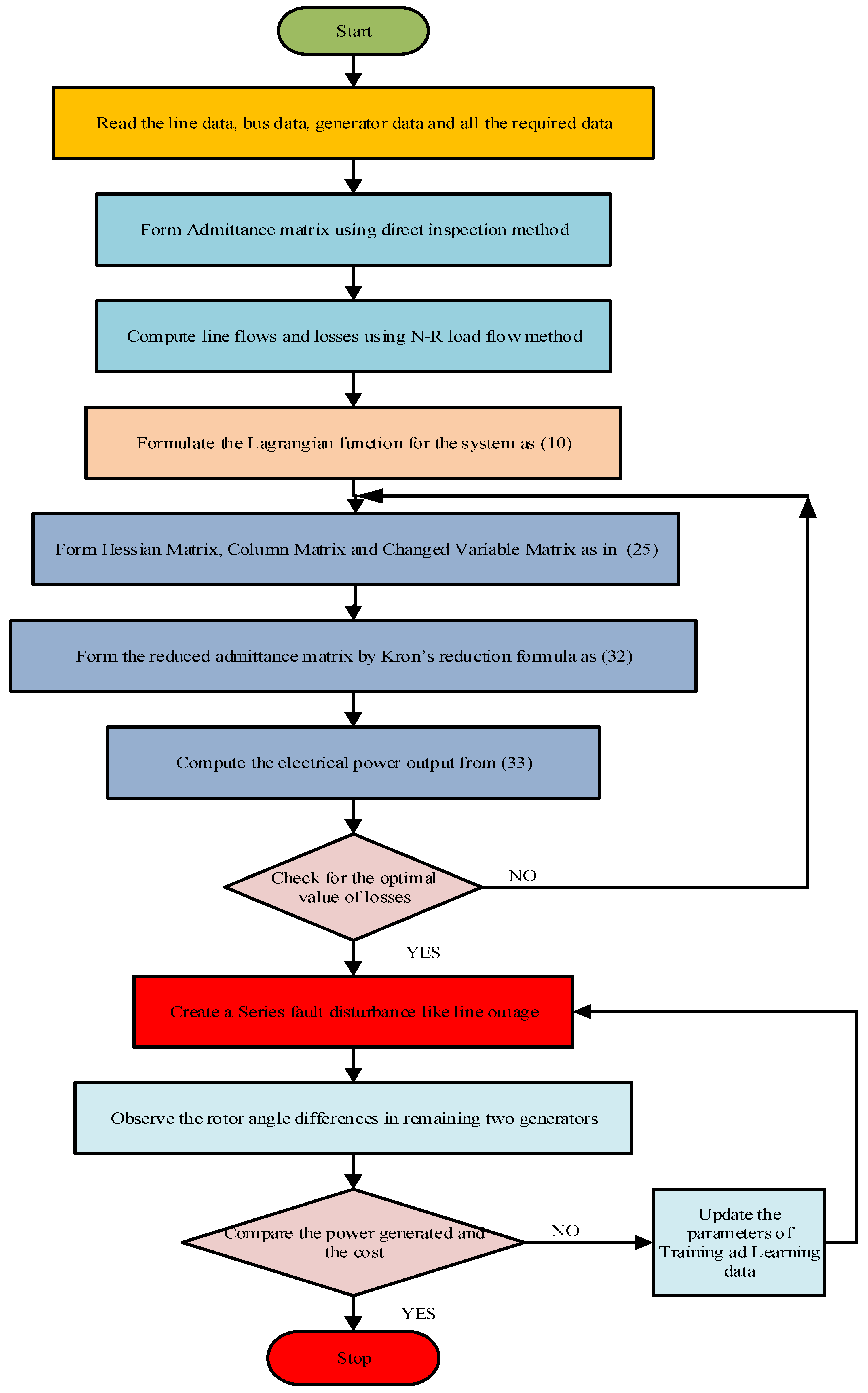Section 6 provides a detailed explanation of the suggested flow chart. Section 7 and Section 8 describe the case study and results, while part 9 offers conclusions.

2. Gradient Method Power Flow

In order to perform the Gradient Method Power Flow, the N-R load flow method is initially performed. The Static Power Flow Equations of any power system are given below as Equations (1) and (2). Active Power $P_i$ at each bus is given by Equation (1).

$$P_i=U_i^2{Y}_{ii}Cos{\theta }_{ii}+{\sum }_{\begin{array}{c}j=1\\ j\ne i\end{array}}^n\left|U_i{U}_j{Y}_{ij}\right|Cos\left({\theta }_{ij}+{\delta }_i-{\delta }_j\right)$$

(1)

Reactive Power $Q_i$ at each bus is given by Equation (2).

$$Q_i=U_i^2{Y}_{ii}Sin{\theta }_{ii}+{\sum }_{\begin{array}{c}j=1\\ j\ne i\end{array}}^n\left|U_i{U}_j{Y}_{ij}\right|Sin\left({\theta }_{ij}+{\delta }_i-{\delta }_j\right)$$

(2)

The elements of Jacobian matrix for N-R load flow method are determined as Equations (3)–(6).

$$\begin{array}{c}{H}_{ii}={\displaystyle \frac{\partial P_i}{\partial {\delta }_i}}=-{\sum }_{\begin{array}{c}j=1\\ j\ne i\end{array}}^n\left|U_i{U}_j{Y}_{ij}\right|Sin\left({\theta }_{ij}+{\delta }_i-{\delta }_j\right)\\ H_{ij}={\displaystyle \frac{\partial P_i}{\partial {\delta }_j}}=U_i{U}_j{Y}_{ij}Sin\left({\theta }_{ij}+{\delta }_i-{\delta }_j\right)\end{array}$$

(3)

$$\begin{array}{c}{N}_{ii}={\displaystyle \frac{\partial P_i}{\partial V_i}}=2U_i{Y}_{ii}Cos{\theta }_{ii}+{\sum }_{\begin{array}{c}j=1\\ j\ne i\end{array}}^n\left|U_j{Y}_{ij}\right|Cos\left({\theta }_{ij}+{\delta }_i-{\delta }_j\right)\\ N_{ij}={\displaystyle \frac{\partial P_i}{\partial V_j}}=U_i{Y}_{ij}Cos\left({\theta }_{ij}+{\delta }_i-{\delta }_j\right)\end{array}$$

(4)

$$\begin{array}{c}{M}_{ii}={\displaystyle \frac{\partial Q_i}{\partial {\delta }_i}}={\displaystyle \sum _{\begin{array}{c}j=1\\ j\ne i\end{array}}^n}\left|U_i{U}_j{Y}_{ij}\right|Cos\left({\theta }_{ij}+{\delta }_i-{\delta }_j\right)\\ M_{ij}={\displaystyle \frac{\partial Q_i}{\partial {\delta }_j}}=-U_i{U}_j{Y}_{ij}Cos\left({\theta }_{ij}+{\delta }_i-{\delta }_j\right)\end{array}$$

(5)

$$\begin{array}{c}{L}_{ii}={\displaystyle \frac{\partial Q_i}{\partial V_i}}=2U_i{Y}_{ii}Sin{\theta }_{ii}+{\displaystyle \sum _{\begin{array}{c}j=1\\ j\ne i\end{array}}^n}\left|U_j{Y}_{ij}\right|Sin\left({\theta }_{ij}+{\delta }_i-{\delta }_j\right)\\ L_{ij}={\displaystyle \frac{\partial Q_i}{\partial V_j}}=U_i{Y}_{ij}Sin\left({\theta }_{ij}+{\delta }_i-{\delta }_j\right)\end{array}$$

(6)

By using the above Equations (3)–(6), the Jacobian matrix can be formed as in (7)

$$\left[\begin{array}{cc}\begin{array}{cc}{H}_{ii}& H_{ij}\\ H_{ji}& H_{jj}\end{array}& \begin{array}{cc}{N}_{ii}& N_{ij}\\ Nji& N_{jj}\end{array}\\ \begin{array}{cc}{M}_{ii}& M_{ij}\\ M_{jj}& M_{jj}\end{array}& \begin{array}{cc}{L}_{ii}& L_{ij}\\ L_{Jj}& L_{jj}\end{array}\end{array}\right]$$

(7)

To obtain the rotor angle or the load angle ($\delta )$ and voltage $(U)$ values multiply the inverse of Jacobian Matrix with the change in P and Q as in Equation (8).

$$\left[\begin{array}{c}\mathsf{\Delta }\delta \\ \mathsf{\Delta }U\end{array}\right]=\left[J^{-1}\right]\left[\begin{array}{c}\mathsf{\Delta }P\\ \mathsf{\Delta }Q\end{array}\right]$$

(8)

Check for the convergence criterion for rotor angle and voltage as in Equation (9)

$${{\delta }^{\prime }}_{new}={\delta }^0+\mathsf{\Delta }{\delta }^0;{U^{\prime }}_{new}=U^0+\mathsf{\Delta }{U}^0$$

(9)

The Lagrangian function for the static power flow expression is given in Equation (10)

$$L(P_{gi},U,\delta )={\sum }_{i=1}^{ng}f(P_{gi})-{\lambda }_{pi}(P_i-P_{gi}+P_{di})-{\lambda }_{qi}(Q_i-Q_{gi}+Q_{di})$$

(10)

Derivate Equation (10) partially twice to obtain the elements of column matrix and the hessian matrix as in Equations (11)–(15). ${\lambda }_{pi}$, ${\lambda }_{qi}$ are the penalty coefficient, and the value of the penalty coefficient is considered as unity.

$${\nabla }_{P_g{P}_g}=2a_i;{\nabla }_{\lambda P_i{P}_{gi}}=-1;{\nabla }_{P_{gi}{\lambda }_{Pi}}=-1;{\nabla }_{\lambda P_j{P}_{gi}}=0;{\nabla }_{\lambda P_i{P}_{gj}}=0;{\nabla }_{P_{gj}{\lambda }_{Pi}}=0$$

(11)

$${\displaystyle \frac{{\partial }^2{P}_i}{\partial {\delta }_i^2}}=-U_i{\sum }_{\begin{array}{c}j=1\\ j\ne i\end{array}}^{NB}{U}_j{Y}_{ij}Cos\left({\theta }_{ij}+{\delta }_i-{\delta }_j\right);{\displaystyle \frac{{\partial }^2{Q}_i}{\partial {\delta }_i^2}}=-U_i{\sum }_{\begin{array}{c}j=1\\ j\ne i\end{array}}^{NB}{U}_j{Y}_{ij}Sin\left({\theta }_{ij}+{\delta }_i-{\delta }_j\right)$$

(12)

$${\displaystyle \frac{{\partial }^2{Q}_i}{\partial {\delta }_j\partial {\delta }_i}}=U_i{U}_j{Y}_{ij}Sin\left({\theta }_{ij}+{\delta }_i-{\delta }_j\right)=-{\displaystyle \frac{{\partial }^2{Q}_i}{\partial {{\delta }_j}^2}}={\displaystyle \frac{{\partial }^2{Q}_i}{\partial {\delta }_i\partial {\delta }_j}}$$

(13)

$${\displaystyle \frac{{\partial }^2{P}_i}{\partial {\delta }_j\partial {\delta }_i}}=U_i{U}_j{Y}_{ij}Cos\left({\theta }_{ji}+{\delta }_i-{\delta }_j\right)=-{\displaystyle \frac{{\partial }^2{P}_i}{\partial {{\delta }_j}^2}}={\displaystyle \frac{{\partial }^2{P}_i}{\partial {\delta }_j\partial {\delta }_i}}$$

(14)

$${\nabla }_{\delta \delta }={\lambda }_{p_i}\left({\sum }_{i=1}^{NS}{\displaystyle \frac{{\partial }^2{P}_i}{\partial {\delta }^2}}\right)+{\lambda }_{q_i}\left({\sum }_{i=NS+1}^{NB}{\displaystyle \frac{{\partial }^2{Q}_i}{\partial {\delta }^2}}\right)$$

(15)

where NS = number of generator buses, NB = total number of buses. The subsequent equations of the Hessian matrix are shown below in Equations (16)–(24)

$${\displaystyle \frac{{\partial }^2{P}_i}{\partial {\delta }_i\partial U_j}}=-U_i{Y}_{ij}Sin\left({\theta }_{ij}+{\delta }_i-{\delta }_j\right);{\displaystyle \frac{{\partial }^2{P}_i}{\partial {\delta }_j\partial Ui}}=U_j{Y}_{ij}Sin\left({\theta }_{ij}+{\delta }_i-{\delta }_j\right)$$

(16)

$${\displaystyle \frac{{\partial }^2{Q}_i}{\partial {\delta }_j\partial U_q}}={\sum }_{j=1}^{NB}{U}_j{Y}_{ij}Cos\left({\theta }_{ij}+{\delta }_i-{\delta }_j\right);{\displaystyle \frac{{\partial }^2{P}_i}{\partial {\delta }_i\partial U_i}}=-U_j{\sum }_{j=1}^{NB}{Y}_{ij}Sin\left({\theta }_{ij}+{\delta }_i-{\delta }_j\right)$$

(17)

$${\displaystyle \frac{{\partial }^2{Q}_i}{\partial U_i\partial {\delta }_i}}={\sum }_{\begin{array}{c}j=1\\ j\ne i\end{array}}^{NB}{U}_j{Y}_{ij}Cos\left({\theta }_{ij}+{\delta }_i-{\delta }_j\right)$$

(18)

$${\nabla }_{\delta U}={\lambda }_{p_i}\left({\sum }_{i=1}^{NS}{\displaystyle \frac{{\partial }^2{P}_i}{\partial \delta \partial U}}\right)+{\lambda }_{q_i}\left({\sum }_{i=NS+1}^{NB}{\displaystyle \frac{{\partial }^2{Q}_i}{\partial \delta \partial U}}\right);{\nabla }_{U\delta }={\nabla }_{\delta U}$$

(19)

$${\displaystyle \frac{{\partial }^2{P}_i}{\partial U_i^2}}=2Y_{ii}Cos\left({\theta }_{ii}\right);{\displaystyle \frac{{\partial }^2{P}_i}{\partial U_j\partial U_i}}=Y_{ji}Cos\left({\theta }_{ij}+{\delta }_i-{\delta }_j\right)$$

(20)

$${\displaystyle \frac{{\partial }^2{Q}_i}{\partial U_i^2}}=2Y_{ii}Sin\left({\theta }_{ii}\right);{\displaystyle \frac{{\partial }^2{Q}_i}{\partial U_j\partial U_i}}=Y_{ji}Sin\left({\theta }_{ij}+{\delta }_i-{\delta }_j\right)$$

(21)

$${\nabla }_{UU}={\lambda }_{p_i}\left({\displaystyle \frac{{\partial }^2{P}_i}{\partial U^2}}\right)+{\lambda }_{q_i}\left({\displaystyle \frac{{\partial }^2{Q}_i}{\partial U^2}}\right)$$

(22)

The second derivative sub-matrices of the Hessian matrix is given as in Equations (23) and (24)

$${\nabla }_{{\lambda }_P\delta }=\left[\begin{array}{cc}{H}_{ii}& H_{ij}\\ H_{ji}& H_{jj}\end{array}\right]={\nabla }_{\delta {\lambda }_p};{\nabla }_{{\lambda }_q\delta }=\left[\begin{array}{cc}{M}_{ii}& M_{ij}\\ M_{ji}& M_{jj}\end{array}\right]={\nabla }_{\delta {\lambda }_q}$$

(23)

$${\nabla }_{{\lambda }_{p}U}=\left[\begin{array}{cc}{N}_{ii}& N_{ij}\\ N_{ji}& N_{jj}\end{array}\right]={\nabla }_{U{\lambda }_p};{\nabla }_{{\lambda }_{q}U}=\left[\begin{array}{cc}{L}_{ii}& L_{ij}\\ L_{ji}& L_{jj}\end{array}\right]={\nabla }_{U{\lambda }_q}$$

(24)

Hessian matrix, Column matrix, and Changed variable matrix is given below as in Equation (25)

$$HM=\left[\begin{array}{ccccc}{\nabla }_{P_g{P}_g}& 0& {\nabla }_{P_g{\lambda }_p}& 0& 0\\ 0& {\nabla }_{\delta \delta }& {\nabla }_{\delta {\lambda }_p}& {\nabla }_{\delta U}& {\nabla }_{\delta {\lambda }_q}\\ {\nabla }_{{\lambda }_p{P}_g}& {\nabla }_{{\lambda }_p\delta }& 0& {\nabla }_{{\lambda }_{p}U}& 0\\ 0& {\nabla }_{U\delta }& {\nabla }_{U{\lambda }_P}& {\nabla }_{UU}& {\nabla }_{U{\lambda }_q}\\ 0& {{\nabla }_{\lambda }}_{q\delta }& 0& {\nabla }_{{\lambda }_{q}U}& 0\end{array}\right];C=\left[\begin{array}{c}-{\nabla }_{P{g}_i}\\ -{\nabla }_{{\delta }_i}\\ -{\nabla }_{{\lambda }_p}\\ -{\nabla }_U\\ -{\nabla }_{{\lambda }_q}\end{array}\right];B=\left[\begin{array}{c}{\mathsf{\Delta }}_{P_{gi}}\\ {\mathsf{\Delta }}_{\delta }\\ {\mathsf{\Delta }}_{{\lambda }_p}\\ {\mathsf{\Delta }}_U\\ {\mathsf{\Delta }}_{{\lambda }_q}\end{array}\right]$$

(25)

The computation of the changed variable matrix can be found as in Equation (26)

$$\left[HM\right]\times \left[B\right]=\left[C\right]\mathrm{results}\mathrm{in}\left[B\right]={\left[HM\right]}^{-1}\times \left[C\right]$$

(26)

Cost functions of the generators are given as below in Equations (27) and (28). The cost coefficients are$a_{in}$, $b_{in},C_{in}$ for the generators.

$$F_1\left(P_{gi}\right)=\left\{\begin{array}{c}{a_{i1}+b_{i1}P}_{gi}+C_{i1}{P}_{gi}^2\\ {a_{i2}+b_{i2}P}_{gi}+C_{i2}{P}_{gi}^2\\ ⋮\\ {a_{in}+b_{in}P}_{gi}+C_{in}{P}_{gi}^2\end{array}\right.`$$

(27)

The objective function for the cost computation is given as in Equation (28):

$$J=\left(\sum _{i=1}^2{a_{in}+b_{in}P}_{gi}+C_{in}{P}_{gi}^2\right)+\left(\sum _{i=3}^{NG}{a_i+b_{i}P}_{gi}+C_i{P}_{gi}^2\right)$$

(28)

3. Formulation for Transient Analysis during Line Outages

The transients occur in the system due to various internal and external disturbances. These various disturbances include single-line outages, double-line outages, and faults in the transformer and on other electrical equipment [26]. The voltage behind transient reactance is given in Equation (29)

$${\mathit{E}}_{\mathit{i}}^{\mathbf{1}}={\mathit{U}}_{\mathit{i}}+\mathit{j}{\mathit{X}}_{\mathit{d}}^{\mathbf{1}}{\mathit{I}}_{\mathit{i}}$$

(29)

Loads are converted into equivalent admittances as in Equations (30) and (31).

$${\mathit{Y}}_{\mathit{i}}={\displaystyle \frac{{\mathit{S}}_{\mathit{i}}^{\mathit{*}}}{{\left|{\mathit{U}}_{\mathit{i}}\right|}^2}}={\displaystyle \frac{{\mathit{P}}_{\mathit{i}}-\mathit{j}{\mathit{Q}}_{\mathit{i}}}{{\left|{\mathit{U}}_{\mathit{i}}\right|}^2}};{\mathit{I}}_{\mathit{b}\mathit{u}\mathit{s}}=\begin{array}{c}\left[{\mathit{Y}}_{\mathit{b}\mathit{u}\mathit{s}}\right]\end{array}{\mathit{U}}_{\mathit{b}\mathit{u}\mathit{s}}$$

(30)

$$\left[\begin{array}{c}\mathbf{0}\\ {\mathit{I}}_{\mathit{m}}\end{array}\right]=\left[\begin{array}{cc}{\mathit{Y}}_{\mathit{n}\mathit{n}}& {\mathit{Y}}_{\mathit{n}\mathit{m}}\\ {\mathit{Y}}_{\mathit{m}\mathit{n}}& {\mathit{Y}}_{\mathit{m}\mathit{m}}\end{array}\right]\left[\begin{array}{c}{\mathit{U}}_{\mathit{n}}\\ {\mathit{E}}_{\mathit{m}}^{\mathbf{1}}\end{array}\right]$$

(31)

By Kron’s reduction formula the reduced admittance matrix is given in Equation (32),

$$Y_{reduced}=Y_{nn}-\left[\begin{array}{c}{Y}_{nm}{[Y_{mm}]}^{-1}{Y}_{mn}\end{array}\right]$$

(32)

Electrical power output can be computed using Equations (33) and (34), the apparent power $S_{ei}^{*}$ is

$${\mathit{S}}_{\mathit{e}\mathit{i}}^{\mathit{*}}={\mathit{E}}_{\mathit{i}}^{\mathit{*}}{\mathit{I}}_{\mathit{i}}$$

(33)

$${\mathit{S}}_{\mathit{e}\mathit{i}}^{\mathit{*}}={\mathit{E}}_{\mathit{i}}^{\mathit{*}}{\mathit{I}}_{\mathit{i}} {\mathit{P}}_{\mathit{e}\mathit{i}}=\mathit{Re}\mathit{a}\mathit{l}\left[{\mathit{E}}_{\mathit{i}}^{\mathit{*}}{\mathit{I}}_{\mathit{i}}\right];{\mathit{I}}_{\mathit{i}}={\sum }_{\mathit{j}=1}^{\mathit{m}}{\mathit{E}}_{\mathit{j}}^1{\mathit{Y}}_{\mathit{i}\mathit{j}}$$

(34)

The electrical active power $P_{ei}$ and the electrical active power at the bus ‘m’ is $P_{mi}$ as given below in Equation (35)

$${\mathit{P}}_{\mathit{e}\mathit{i}}={\sum }_{\mathit{j}=1}^{\mathit{m}}\left|{\mathit{E}}_{\mathit{i}}^1\right|\left|{\mathit{E}}_{\mathit{j}}^1\right|\left|{\mathit{Y}}_{\mathit{i}\mathit{j}}\right|\mathit{C}\mathit{o}\mathit{s}\left({\mathit{\theta }}_{\mathit{i}\mathit{j}}+{\mathit{\delta }}_{\mathit{i}}-{\mathit{\delta }}_{\mathit{j}}\right);{\mathit{P}}_{\mathit{m}\mathit{i}}={\sum }_{\mathit{j}=1}^{\mathit{m}}\left|{\mathit{E}}_{\mathit{i}}^1\right|\left|{\mathit{E}}_{\mathit{j}}^1\right|\left|{\mathit{Y}}_{\mathit{i}\mathit{j}}\right|\mathit{C}\mathit{o}\mathit{s}\left({\mathit{\theta }}_{\mathit{i}\mathit{j}}+{\mathit{\delta }}_{\mathit{i}}-{\mathit{\delta }}_{\mathit{j}}\right)$$

(35)

4. Modification in Bus Admittance Matrix

Variation in the bus admittance ($Y_{bus}$) matrix plays a key role in the analysis of the transient stability of a power system [27]. The different cases considered for the modification of $Y_{bus}$ matrix during the analysis of transient stability are given below.

• In conventional $Y_{bus}$, the generator reactances are not considered. But, in the transient stability analysis, they are considered by converting them to respective admittances.
• The load admittances are considered by converting the load into admittance using Equation (30).
• If a bus has both generator and load, the admittances of both generator and load are added to the self-admittance values.
• The size of $Y_{bus}$ is increased by the total number of generators presented in the system.
• Kron’s reduction formula is used to reduce the size of the admittance matrix, as in Equation (32).

In each case, the mechanical power before fault, during fault, and after fault are calculated, and the critical clearing angle at each bus is calculated by using Equation (36)

$${\delta }_c=Co{s}^{-1}\left(\left(\left({\delta }_m-{\delta }_0\right){\mathit{sin\delta }}_0-r_{1}Cos{\delta }_0+r_{2}Cos{\delta }_m\right)/\left(r_2-r_1\right)\right)$$

(36)

These critical angle values are obtained and are incorporated in the Gradient Method Power Flow values and Gradient Method Power Flow is performed to gain Transient Constrained GMPF.

5. Training-Learning Based Optimization Algorithm

Optimizing the parameters is crucial for fine-tuning the algorithm under suitable conditions. The algorithms’ performance is typically impacted by this. Inadequate adjustment of algorithm-specific parameters either results in a locally optimal solution or increases computational work. Additionally, common control parameters must be adjusted, adding to the effort. Teaching-learning-based optimization (TLBO) is an algorithm that satisfies this requirement by not requiring any algorithm-specific parameters.

TLBO algorithm is classified into two phases as follows:

• Trainers’s phase
• Learner’s phase

5.1. Trainers Phase

This is the main part of the algorithm where students receive the knowledge from the instructor. Depending on their abilities, trainers attempt to raise the class mean in the subject they are teaching throughout this period. The best learner recognized by the algorithm is regarded as the trainer; trainers are typically thought of as highly educated individuals who mentor students to help them achieve better outcomes. The discrepancy between the trainer’s corresponding performance for each subject and the current mean result for each subject is represented by Equation (37)

$$D{M}_{jj,k,ww}=r_{ww}\left(X_{jj,k_{best},ww}-T_F{M}_{jj,ww}\right)$$

(37)

$T_F$ is the teaching factor which decides the value of mean to be changed, and $r_{ww}$ is the random number in the range [0, 1]. Value of $T_F$ can be either 1 or 2. The value of $T_F$ is decided randomly with equal probability as Equation (38) and is chosen 1 or 2 as the difference mean and provides the better value

$$T_F=round\left[1+rand\left(\mathrm{0,1}\right)\left\{2,-1\right\}\right]$$

(38)

Based on $D{M}_{jj,k,ww}$, the current solution is reorganized in the trainer phase according to the Equation (39).

$$X_{jj,k,ww}^{\prime }=X_{jj,k,ww}+D{M}_{jj,k,ww}$$

(39)

5.2. Learners Phase

In this second stage of the algorithm, students interact with one another to expand their knowledge. In order to expand their knowledge, students engage in sporadic interactions with other students. When another learner is more knowledgeable than the learner, the learner gains new information.

Let $g,h$ are two random learners, such that $X_{total-g,jj}^{\prime }\ne X_{total-h,jj}^{\prime }$

$${X^{\left|\right|}}_{jj,g,ww}={X^{|}}_{jj,g,ww}+r_{ww}\left({X^{|}}_{jj,g,ww}-{X^{|}}_{jj,h,ww}\right),\mathrm{if}{X}_{total-g,ww}^{\prime }<X_{total-h,ww}^{\prime }$$

(40)

$${X^{\left|\right|}}_{jj,g,ww}={X^{|}}_{jj,g,ww}+r_{ww}\left({X^{|}}_{jj,h,ww}-{X^{|}}_{jj,g,ww}\right),\mathrm{if}{X}_{total-g,ww}^{\prime }>X_{total-h,ww}^{\prime }$$

(41)

${X^{\left|\right|}}_{jj,g,ww}$ is accepted if it provides better a best value.

The minimization problems are handled by (40) and (41). The applications of Equations (42) and (43) are to maximize issues.

$${X^{\left|\right|}}_{jj,g,ww}={X^{|}}_{jj,g,ww}+r_{ww}\left({X^{|}}_{jj,g,ww}-{X^{|}}_{jj,h,ww}\right),\mathrm{if}{X}_{total-g,ww}^{\prime }>X_{total-h,ww}^{\prime }$$

(42)

$${X^{\left|\right|}}_{jj,g,ww}={X^{|}}_{jj,g,ww}+r_{ww}\left({X^{|}}_{jj,h,ww}-{X^{|}}_{jj,g,ww}\right),\mathrm{if}{X}_{total-g,ww}^{\prime }<X_{total-h,ww}^{\prime }$$

(43)

The implement the TLBO algorithm for both minimization and maximization problems has been developed by the above equations, respectively.

6. Flow Chart of the Proposed Research

The flow chart of the proposed research is shown in Figure 2. It explains the steps involved in the analysis of transient stability through optimization. It starts from the read-the-line data, bus data, and generator data, forming the admittance matrix with the direct inspection method, computing the line flow and losses using Newton–Rapson method, formulating the Lagrangian function for Equation (10), forming the Hessian Matrix, Column Matrix and Changed Variable Matrix, forming the reduced admittance matrix, computing the electrical power output, checking for the optimal value of losses, creating a line outage, observing the root angle differences in remaining two generators, comparing the power generated and the cost and updating the parameters of training and learning data.

7. Case Study and Results

A typical 3-machine, 5-bus system has been used to test the proposed algorithm. This system comprises three generator buses, two load buses, and seven transmission lines. The NR load flow technique calculates the Regular Power Flow (RPF). It was utilized in comparison with the Gradient Method Power Flow (GMPF). The value of the cost coefficient for three generators is given in

Table 1. Cost coefficient for three generators.

Generation Bus No.	a	b	c
1	60	200	140
2	75	150	120
3	70	180	80

.

Table 2. Comparison of transmission line flow through RPF and GMPF.

Line No.	From Bus	To Bus	P (MW)		Q (MVAR)
			RPF	GMPF	RPF	GMPF
1	1	2	27.11	0.85	−29.73	−5.06
2	1	3	14.09	0.01	−7.25	−2.22
3	2	3	9.89	0.27	0.42	−0.99
4	2	4	16.23	8.46	0.06	−0.67
5	2	5	49.58	45.67	4.67	5.91
6	3	4	37.65	49.11	−3.83	1.1
7	4	5	12.5	16.4	−1.69	0.39

shows the ideal power flow without considering the transient stability condition and without using the TLBO method and the active and reactive power flow of the normal power flow technique. According to the table, the regular technique’s active and reactive power flows are greater than those of the optimal power flow approach.

The total system losses are given below in

Table 3. Total system losses for power flow technique and optimal power flow technique.

System Losses	P (MW)		Q (MVAR)
	RPF	GMPF	RPF	GMPF
	1.719	1.589	5.16	4.77

. It can be seen that the total system losses in terms of active power have been reduced to about 0.15 MW, and in terms of reactive power, the reduction is 0.9 MVAR.

Depending on the objective function, the TLBO algorithm has been developed and compared with the regular GMPF method. The results are shown in

Table 4. Comparison of active power generation.

Generation Bus No.	RPF	GMPF
1	54.41	53.59
2	51.92	48.58
3	65.12	64.76

.

The transient stability analysis was considered in 10 cases, as given below:

Case-1: Bus-1 issue and the time it takes to clear it of 0.01 s.

Case-2: Bus-1 issue and the time it takes to clear it of 0.25 s.

Case-3: Bus-2 issue and the time it takes to clear it of 0.1 s.

Case-4: Bus-2 issue and the time it takes to clear it of 0.25 s.

Case-5: Bus-3 issue and the time it takes to clear it of 0.1 s.

Case-6: Bus-3 issue and the time it takes to clear it of 0.25 s.

Case-7: Bus-4 issue and the time it takes to clear it of 0.1 s.

Case-8: Bus-4 issue and the time it takes to clear it of 0.25 s.

Case-9 Bus-5 issue and the time it takes to clear it of 0.1 s.

Case-10: Bus-5 issue and the time it takes to clear it of 0.25 s.

7.1. Case-1: Bus-1 Issue and the Time It Takes to Clear It of 0.01 s

In this instance, a defect is established at bus1, with a final time of 2 s and a fault clearing time of 0.01 s. Figure 3 shows the phase angle difference for the line-1 between the bus-1 and bus-2 outages.

The fault clearing time of 0.01 s within which a fault must be cleared to maintain system stability. If the fault is not cleared within this time, the system may become unstable, leading to severe consequences like cascading failures. At the fault clearing time of 0.01 s, the critical clearing angle is determined to be −1.3040, −4.0534. These angles represent the maximum permissible angle displacement (in degrees) at which the system can still maintain stability after a fault occurs. The negative values indicate that the system is already under strain, and the smaller the negative angle, the closer the system is to becoming unstable. A more negative critical clearing angle implies a higher risk of instability, meaning the system must clear the fault very quickly to avoid an unstable situation. This angle is considered when transients occur in the system.

Table 5. Comparison of active power generation.

Generation Bus No.	DSCGMPF	TLBODSCGMPF
1	54.46	53.59
2	51.97	48.58
3	65.18	64.76

provides the active power generation. For generator-1, the DSCGMPF method produces slightly more power than TLBODSCGMPF, with a difference of 0.87 MW. This indicates marginally higher generation efficiency at this bus under DSCGMPF. For generator-2, the DSCGMPF method generates 3.39 MW more power than TLBODSCGMPF, showing a more significant difference compared to Bus 1. This suggests that the DSCGMPF method is notably more effective at this bus in terms of power generation. For generator-3, the difference here is minimal, with DSCGMPF producing only 0.42 MW more than TLBODSCGMPF. This suggests that at Bus 3, both methods are almost equally effective in power generation.

Table 6. Comparison of Generation Cost ($/h).

DSCGMPF	TLBODSCGMPF
696,020.75	350,983.9

provides the generating cost ($/h). The DSCGMPF method, while generally producing more power, is significantly more expensive, with almost double the generation cost compared to TLBODSCGMPF. This high cost may be due to several factors, such as higher fuel costs, more expensive technology, or inefficiencies in operation despite the higher power output. In contrast, TLBODSCGMPF, though producing slightly less power, is much more cost-effective. This makes it a potentially better choice for operations where cost savings are prioritized over maximizing power output.

7.2. Case-2: Bus-1 Issue and the Time It Takes to Clear It of 0.25 s

In this instance, a fault is formed at bus1, and the final time is 2 s, with a fault clearance time of 0.25 s. Figure 4 shows the phase angle difference for the line-1 between the bus-1 and bus-2 outages.

The fault clearing time is 0.25 s, within which a fault in the power system must be cleared to prevent system instability. The critical clearing angles, −5.9402 and −17.754, are indicative of the system’s stability limits. These angles are key in determining the system’s ability to return to a stable operating condition post-fault. The negative values suggest that the system is potentially unstable or operating under conditions that could lead to instability during transients.

Table 7. Comparison of active power generation.

Generation Bus No.	DSCGMPF	TLBODSCGMPF
1	55.31	53.98
2	52.80	48.98
3	66.21	64.54

provides the active power generation. DSCGMPF is a strategy that involves advanced control techniques to distribute power generation more effectively. TLBODSCGMPF method likely incorporates the optimization of transmission line losses and better distribution. Across all buses, TLBODSCGMPF results in slightly lower active power generation compared to DSCGMPF. This reduction in power generation might indicate more efficient power distribution or reduced losses in the system.

Table 8. Comparison of Generation Cost ($/h).

DSCGMPF	TLBODSCGMPF
717,737.02	352,186.9

provides the generating cost ($/h). The TLBODSCGMPF method significantly reduces the generation cost compared to DSCGMPF. The cost reduction could be attributed to improved efficiency in power distribution, better loss management, and optimal control of generation resources.

7.3. Case-3: Bus-2 Issue and the Time It Takes to Clear It of 0.1 s

In this instance, a fault is generated at bus2, with a final time of 2 s and a fault clearing time of 0.1 s. Figure 5 shows the phase angle difference for the line-1 between the bus-1 and bus-2 outages.

At the fault clearing time of 0.1 s, the crucial clearing angle is taken into consideration as 8.2201, −4.0557. The values 8.2201 and −4.0557 are crucial angles, likely representing the maximum and minimum permissible angles before the system loses synchronism. These angles are important in transient stability analysis, which ensures the system remains stable after a fault is cleared. This clearing angle is critical during transient conditions (like a fault). If the fault is not cleared within this angle range, the system could experience instability, leading to potential outages or damage to equipment.

Table 9. Comparison of active power generation.

Generation Bus No.	DSCGMPF	TLBODSCGMPF
1	55.38	55.68
2	52.87	50.68
3	66.30	62.47

provides the active power generation. For generator-1, the TLBODSCGMPF method results in slightly higher power generation compared to DSCGMPF (+0.30 MW). For generator-2 and 3, TLBODSCGMPF results in lower power generation compared to DSCGMPF, with Bus 2 showing a reduction of 2.19 MW and Bus 3 a reduction of 3.83 MW. The TLBODSCGMPF method seems to slightly increase generation at Bus 1 but reduces it at Buses 2 and 3. This could indicate a redistribution of generation to achieve some optimization criteria, possibly related to cost, losses, or stability.

Table 10. Comparison of Generation Cost ($/h).

DSCGMPF	TLBODSCGMPF
719,576.63	355,717.5

provides the generation cost ($/h). This represents the cost of generating power using the two different methods. Lower costs are generally preferred as they imply more efficient or economically optimal operation. DSCGMPF has a much higher generation cost ($719,576.63 per hour). Meanwhile, TLBODSCGMPF gives significantly lower generation costs ($355,717.50 per hour), which is almost half of the DSCGMPF method. The TLBODSCGMPF method is much more cost-effective compared to the DSCGMPF method, which suggests it may be a more optimized approach in terms of economic dispatch or cost minimization.

7.4. Case-4: Bus-2 Issue and the Time It Takes to Clear It of 0.25 s

Here, a fault forms at bus 2, and the fault clearing time is 0.25 s, with a final time of 2 s. The phase angle discrepancy for line-1 between the bus-1 and bus-2 outages is displayed in Figure 6.

The fault clearing time of 0.25 s is the time within which a fault must be cleared to avoid instability in the power system. A longer clearing time (0.25 s compared to the previous 0.01 s) indicates that the system can tolerate faults for a longer duration before becoming unstable. The positive angle is significant at 58.1979°. It suggests that the system can handle a considerable phase displacement before it reaches the point of instability when the fault is cleared in 0.25 s. The system is more stable under these conditions compared to the earlier scenario with a critical clearing angle of −1.3040°. The value −4.1886° is the negative angle, slightly more negative than before, and represents the margin at which the system may begin to become unstable if not cleared appropriately. The system exhibits more resilience to transients with a fault clearing time of 0.25 s, given the larger positive critical clearing angle. However, the presence of a negative critical clearing angle indicates that the system’s stability is still a concern and needs careful management, especially at specific points in the network.

Table 11. Comparison of active power generation.

Generation Bus No.	DSCGMPF	TLBODSCGMPF
1	78.55	70.05
2	75.83	74.3
3	93.98	91.72

provides the active power generation. For generator-1, DSCGMPF produces 8.5 MW more power than TLBODSCGMPF. This significant difference indicates a stronger generation capability for DSCGMPF at this bus. For generator-2, the difference here is 1.53 MW, with DSCGMPF again generating more power. However, the difference is smaller compared to Bus 1, suggesting a more comparable performance between the two methods on this bus. For generator-3, the DSCGMPF method generates 2.26 MW more power than TLBODSCGMPF. While DSCGMPF still leads, the difference is moderate.

Table 12. Comparison of Generation Cost ($/h).

DSCGMPF	TLBODSCGMPF
1,437,799.92	448,156.8

provides the generating cost ($/h). DSCGMPF incurs a significantly higher generation cost, over three times that of TLBODSCGMPF. Despite the higher power output, the cost-effectiveness of DSCGMPF comes into question due to the substantial difference in costs. This higher expense might be due to more advanced technology, higher operational costs, or inefficiencies that, despite the higher output, result in less favorable economic performance.

7.5. Case-5: Bus-3 Issue and the Time It Takes to Clear It of 0.1 s

In this instance, a defect is formed at bus-3, and the final time is 2 s, whereas the fault clearing time is 0.1 s. Figure 7 below shows the phase angle difference for line-1 between bus-1 and bus-2 outage. The phase angle difference of each machine with respect to the slack bus when the fault is created at bus-3 and the fault clearing time is 0.1 s in degree is 0.2199 and −0.4614.

This angle is considered when transients occur in the system.

Table 13. Comparison of active power generation.

Generation Bus No.	DSCGMPF	TLBODSCGMPF
1	54.41	53.96
2	51.93	50.96
3	65.12	64.5

provides the active power generation. For generator-1, the DSCGMPF method generates 0.45 MW more power than TLBODSCGMPF at this bus. The difference is minimal, indicating that both methods perform similarly in terms of power generation at this bus. For generator-2, DSCGMPF generates 0.97 MW more power than TLBODSCGMPF at this bus. This difference, though still modest, is slightly more pronounced than at Bus 1, showing a slight edge for DSCGMPF in efficiency. For generator-3, DSCGMPF produces 0.62 MW more power than TLBODSCGMPF at this bus. Like the other buses, the difference is small, indicating comparable performance between the two methods. The power generation differences between DSCGMPF and TLBODSCGMPF are relatively small across all buses, suggesting that both methods are closely matched in terms of efficiency. DSCGMPF consistently generates slightly more power, but the differences are not substantial, indicating that TLBODSCGMPF could be a viable alternative depending on other factors, such as cost.

Table 14. Comparison of Generation Cost ($/h).

DSCGMPF	TLBODSCGMPF
694,862.99	353,962.2

provides the generating cost ($/h). The generation cost for DSCGMPF is nearly double that of TLBODSCGMPF despite the slight increase in power generation. This significant cost difference suggests that while DSCGMPF may offer a marginal increase in power output, it does so at a much higher expense. The efficiency gains in power generation may not justify the additional cost, depending on the priorities of the system.

7.6. Case-6: Bus-3 Issue and the Time It Takes to Clear It of 0.25 s

In this instance, a fault is formed at bus 3, with a 0.25-second fault clearing time and a 2-second final time. Figure 8 shows the phase angle difference for line-1 between the bus-1 and bus-2 outages. The fault clearance time of 0.25 s is the time within which a fault must be cleared to maintain system stability. A fault clearing time of 0.25 s suggests that the system can tolerate a fault for this duration before it risks becoming unstable. The positive angle is 6.1595°, indicating that the system can handle a small phase displacement before becoming unstable. This angle is less than the 58.1979° angle you provided earlier, suggesting slightly lower stability but still within a stable range. The positive angle is 17.9293° and is larger than 6.1595°, suggesting that the system remains stable under a broader range of conditions when this angle is reached. The system exhibits resilience to transients within the range of these angles, though the larger angle (17.9293°) suggests a greater tolerance before instability occurs. These angles indicate that the system should manage transients well within the fault clearance time of 0.25 s.

Table 15. Comparison of active power generation.

Generation Bus No.	DSCGMPF	TLBODSCGMPF
1	55.30	53.1
2	52.80	51.46
3	66.21	64.46

provides the active power generation. For generator-1, DSCGMPF generates 2.2 MW more power than TLBODSCGMPF at this bus. This indicates a modest efficiency gain for DSCGMPF in power generation. For generator-2, the difference here is 1.34 MW, with DSCGMPF again producing more power. The gap is smaller than in Bus 1 but still shows a consistent advantage for DSCGMPF. For generator-3, the DSCGMPF method generates 1.75 MW more power than TLBODSCGMPF at this bus. This is the largest power output among the three buses for both methods, indicating the importance of this bus in the overall power generation strategy.

Table 16. Comparison of Generation Cost ($/h).

DSCGMPF	TLBODSCGMPF
717,612.71	352,920.1

provides the generating cost ($/h). DSCGMPF incurs a much higher generation cost, more than double that of TLBODSCGMPF. Despite the increased power generation, the cost difference raises concerns about the economic efficiency of DSCGMPF. The cost of producing the additional power with DSCGMPF is significantly higher, making it a less attractive option if cost minimization is a priority.

7.7. Case-7: Bus-4 Issue and the Time It Takes to Clear It of 0.1 s

In this instance, a fault is formed at bus4, with a final time of 2 s and a fault clearing time of 0.01 s. Figure 9 shows the phase angle difference for the line-1 between the bus-1 and bus-2 outages.

At the fault clearing time of 0.1 s, a shorter fault clearing time indicates a more sensitive system that requires a quicker response to avoid instability. The system must clear faults within this time frame to maintain stability. The slightly negative angle −0.0937°, suggests that the system is on the verge of instability and can tolerate only a minimal phase displacement before becoming unstable. The more negative angle −2.1898°, indicates an even narrower margin for maintaining stability during transients. The system’s tolerance for phase displacement is very limited. The negative critical clearing angles at 0.1 s highlight a system that is quite sensitive to transients, requiring rapid fault clearing to avoid instability. The narrow margin for stability indicates that the system is operating close to its limits, and small disturbances could lead to instability if not addressed promptly.

The generation of active power is provided in

Table 17. Comparison of active power generation.

Generation Bus No.	DSCGMPF	TLBODSCGMPF
1	54.44	51.99
2	51.95	50.18
3	65.15	62.34

. For generator-1, DSCGMPF generates 2.45 MW more power than TLBODSCGMPF, showing a notable advantage in power output. For generator-2, the difference here is 1.77 MW, again with DSCGMPF leading. This further emphasizes DSCGMPF’s efficiency in generating more power. For generator-3, DSCGMPF produces 2.81 MW more power than TLBODSCGMPF. This is the largest difference among the buses, suggesting that DSCGMPF is particularly advantageous for this bus. DSCGMPF consistently generates more power than TLBODSCGMPF across all buses, with differences ranging from 1.77 MW to 2.81 MW. This consistent advantage indicates that DSCGMPF is more effective at optimizing power output.

The generation cost ($/h) is provided in

Table 18. Comparison of Generation Cost ($/h).

DSCGMPF	TLBODSCGMPF
695,503.75	349,008.9

. The generation cost for DSCGMPF is nearly double that of TLBODSCGMPF. Despite the higher power output, the cost difference raises concerns about the economic efficiency of DSCGMPF. TLBODSCGMPF, while generating slightly less power, offers a much lower operational cost, making it the more cost-effective option if reducing expenses is a priority.

7.8. Case-8: Bus-4 Issue and the Time It Takes to Clear It of 0.25 s

In this instance, a fault is formed at bus 4, with a 0.25-second fault clearing time and a 2-second final time. Figure 10 shows the phase angle difference for the line-1 between the bus-1 and bus-2 outages.

A fault clearing time of 0.25 s is generally considered a typical duration, providing a balanced response time to clear faults and maintain system stability. The angle, 4.6670°, suggests a moderate tolerance for phase displacement before the system risks instability. The higher angle, 6.6242°, indicates a wider range of stability, allowing the system to manage larger transients without becoming unstable. The system demonstrates a reasonable tolerance for transients within these angles, indicating that it can handle a fair amount of phase displacement without losing stability. The ratio of these angles reflects the system’s ability to maintain stability under varying conditions, providing a buffer against potential instability.

Table 19. Comparison of active power generation.

Generation Bus No.	DSCGMPF	TLBODSCGMPF
1	54.43	51.49
2	51.95	49.07
3	65.15	62.89

provides the active power generation. For generator-1, DSCGMPF generates 2.94 MW more power than TLBODSCGMPF, indicating a notable efficiency advantage. For generator-2, the difference here is 2.88 MW, with DSCGMPF again showing superior power generation capabilities. For generator-3, DSCGMPF produces 2.26 MW more power than TLBODSCGMPF, continuing the trend of higher power output. DSCGMPF consistently generates more power across all buses than TLBODSCGMPF. The differences, ranging from 2.26 MW to 2.94 MW, suggest that DSCGMPF is more effective in maximizing power generation. This consistent superiority highlights DSCGMPF’s efficiency in utilizing the generation capacity at each bus.

Table 20. Comparison of Generation Cost ($/h).

DSCGMPF	TLBODSCGMPF
695,417.20	347,777.4

provides the generating cost ($/h). The generation cost for DSCGMPF is significantly higher than that of TLBODSCGMPF, nearly doubling the cost. While DSCGMPF provides higher power output, the cost difference is substantial, indicating lower economic efficiency. TLBODSCGMPF offers a much lower operation cost, making it a more cost-effective option. Even though it generates less power, the cost savings may outweigh the benefits of the additional power produced by DSCGMPF, especially in cost-sensitive scenarios.

7.9. Case-9 Bus-5 Issue and the Time It Takes to Clear It of 0.1 s

The fault clearing time in this instance is 0.1 s, and the final time is 2 s. The fault is caused by bus 5. Figure 11 provides the phase angle difference for line-1 between bus-1 and bus-2 outages.

The crucial clearing angle is −0.5818, −4.3504, at the fault clearance duration of 0.1 s. A shorter fault-clearing time necessitates prompt fault detection and clearance to avoid instability. The slightly negative angle −0.5818°, indicates a narrow margin for phase displacement before instability occurs. The system is very sensitive to changes, with minimal tolerance for disturbances. The more negative angle −4.3504°, suggests an even narrower stability margin, emphasizing the system’s high sensitivity to disturbances and the need for rapid fault clearing. The system has very tight stability margins at a fault clearing time of 0.1 s. The negative angles indicate that any phase displacement or transient will need to be managed very carefully to maintain system stability. Prompt and effective fault clearance is crucial.

Table 21. Comparison of active power generation.

Generation Bus No.	DSCGMPF	TLBODSCGMPF
1	54.50	51.79
2	52.01	49.03
3	65.23	62.85

shows active power generation, which is considered while analyzing the angle of transients in the system. For generator-1, DSCGMPF generates 2.71 MW more power than TLBODSCGMPF, showing a notable increase in power output. For generator-2, DSCGMPF produces 2.98 MW more power than TLBODSCGMPF, continuing the trend of higher power output. For generator-3, DSCGMPF provides 2.38 MW more power than TLBODSCGMPF, maintaining a consistent advantage across the buses. DSCGMPF shows consistently higher power generation across all buses compared to TLBODSCGMPF, with differences ranging from 2.38 MW to 2.98 MW. This indicates a strong performance in maximizing power output with DSCGMPF.

Table 22. Comparison of Generation Cost ($/h).

DSCGMPF	TLBODSCGMPF
697,106.63	347,514.3

provides the generating cost ($/h). The cost of generating power with DSCGMPF is significantly higher than that of TLBODSCGMPF, nearly double the cost. While DSCGMPF provides greater power output, its economic efficiency is much lower than that of TLBODSCGMPF. TLBODSCGMPF offers a much lower operational cost, making it more attractive from a cost perspective. Despite generating less power, the substantial cost savings may be a critical factor in the decision-making process.

7.10. Case-10: Bus-5 Issue and the Time It Takes to Clear It of 0.25 s

This instance involves the creation of a fault at bus-5, with a 0.25-s fault clearing time and a 2-second final time. In Figure 12, the phase angle difference for line-1 between bus-1 and bus-2 outages is displayed.

The time frame allows for the system to clear faults while maintaining stability, but it’s important to evaluate how well the system handles transients within this duration. At the 0.25-second fault clearing time, the crucial clearing angle is 1.2840, −5.2863. The positive angle 1.2840°suggests that the system has moderate tolerance for phase displacement before it risks becoming unstable. It indicates that the system can handle small to moderate disturbances without immediate instability. The negative angle −5.2863° indicates a relatively large tolerance for disturbances, allowing for a broader range of phase displacement before instability occurs. The larger magnitude of this angle suggests better tolerance to transients. The system has a balanced margin for stability with these critical angles. The positive angle (1.2840°) shows that it can manage small disturbances, while the larger negative angle (−5.2863°) suggests a more robust tolerance for larger disturbances or transients. Overall, the system appears to have a reasonable tolerance for transients during a 0.25-s fault clearing time.

The active power generation is provided in

Table 23. Comparison of active power generation.

Generation Bus No.	DSCGMPF	TLBODSCGMPF
1	54.69	51.2
2	52.20	52.28
3	65.46	62.56

. For generator-1, DSCGMPF generates 3.49 MW more power than TLBODSCGMPF, showing a significant advantage in power output. For generator-2, the power generation is nearly identical, with TLBODSCGMPF slightly ahead by 0.08 MW. The difference is minimal, indicating similar performance on this bus. For generator-3, DSCGMPF produces 2.90 MW more power than TLBODSCGMPF, maintaining a consistent advantage in power generation. DSCGMPF demonstrates superior power generation compared to TLBODSCGMPF at most buses, with differences ranging from 2.90 MW to 3.49 MW. The exception is Generation Bus No. 2, where the power output is nearly the same for both methods. DSCGMPF’s higher power generation across most buses suggests better efficiency in utilizing generation capacity.

The Generation Cost ($/h) is provided in

Table 24. Comparison of Generation Cost ($/h).

DSCGMPF	TLBODSCGMPF
701,851.05	350,626.4

. DSCGMPF incurs a significantly higher cost compared to TLBODSCGMPF, which is nearly double the expense. This higher cost is associated with the increased power output provided by DSCGMPF. TLBODSCGMPF offers a more economical solution with lower operational costs. The substantial cost savings make it the more cost-effective option despite slightly lower power generation in some cases.

8. Conclusions

This study introduces a novel approach for optimal power flow (OPF) by incorporating transient stability constraints into the conventional OPF framework using the Teaching-Learning-Based Optimization (TLBO) method. The proposed Dynamic Stability-Constrained Generation Minimization Power Flow (DSCGMPF) approach ensures that the power system remains transiently stable following contingencies. By integrating dynamic security constraints with static security measures in the TSCOPF (Transient Security-Constrained Optimal Power Flow) formulation, the method addresses both static and dynamic security aspects.

The primary objective of this study was to minimize fuel generation costs while maintaining system stability. The DSCGMPF approach, utilizing TLBO, has proven to be intuitive, reliable, and straightforward. The analysis demonstrates that DSCGMPF effectively achieves the lowest generation fuel costs while adhering to stability constraints during emergency scenarios. This methodology offers a robust solution for optimizing power flow in power systems, ensuring both cost-efficiency and stability.