Multi-Objective Energy Management in Microgrids: Improved Honey Badger Algorithm with Fuzzy Decision-Making and Battery Aging Considerations

Abstract

A multi-objective energy management and scheduling strategy for a microgrid comprising wind turbines, solar cells, fuel cells, microturbines, batteries, and loads is proposed in this work. The plan uses a fuzzy decision-making technique to reduce pollution emissions, battery storage aging costs, and operating expenses. To be more precise, we applied an improved honey badger algorithm (IHBA) to find the best choice variables, such as the size of energy resources and storage, by combining fuzzy decision-making with the Pareto solution set and a chaotic sequence. We used the IHBA to perform single- and multi-objective optimization simulations for the microgrid’s energy management, and we compared the results with those of the conventional HBA and particle swarm optimization (PSO). The results showed that the multi-objective method improved both goals by resulting in a compromise between them. On the other hand, the single-objective strategy makes one goal stronger and the other weaker. Apart from that, the IHBA performed better than the conventional HBA and PSO, which also lowers the cost. The suggested approach beat the alternative tactics in terms of savings and effectively reached the ideal solution based on the Pareto set by utilizing fuzzy decision-making and the IHBA. Furthermore, compared with the scenario without this cost, the results indicated that integrating battery aging costs resulted in an increase of 7.44% in operational expenses and 3.57% in pollution emissions costs.

1. Introduction

1.1. Motivation and Background

With the depletion of fossil fuels, rising energy costs, improved living conditions, environmental concerns, and global warming, the advancement of technology and the adoption of renewable energy sources have seen significant growth in recent years [1]. To mitigate fossil fuel consumption and reduce pollution, it is critical to advance renewable power sources like photovoltaic (PV) systems and miniature wind turbines (WTs). However, the output power of these renewable sources is highly dependent on their geographic location and weather conditions, leading to fluctuations in their energy production [2]. In order to overcome these obstacles, researchers have proposed the concept of a renewable-energy-based electricity microgrid (MG) [3]. The MGs not only contribute to solving environmental issues but also have the potential to transform the technological and economic structures of existing power networks, thereby facilitating the incorporation of green energy sources into the electrical system [3]. Despite the numerous benefits of MGs, their implementation in current distribution networks faces several operational challenges, including issues related to control, security, reliability, flexibility, energy management, and ecological impact [4].

One of the essential aspects of establishing an MG, whether isolated or grid-connected, is maintaining the balance between energy supply and demand. A crucial element in ensuring efficient operation is the energy management system (EMS) [5]. The primary objective of an MG EMS is to deliver power at the lowest possible cost while optimally responding to load demands and supply conditions. To accomplish this, the EMS can conduct real-time energy forecasting for renewable resources, manage energy storage components, and adjust loads to support effective short-term planning and reduce overall operating costs [6]. Additionally, the EMS aims to maximize revenue from each MG resource, ultimately reducing overall power costs. It ensures the MG operates efficiently and cost-effectively, enhancing its long-term sustainability and viability. Meta-heuristic optimization algorithms are vital for energy management in MGs, particularly in optimizing the sizing of energy resources and storage capacity [5,6]. These algorithms provide robust solutions to the complex, multi-objective challenges inherent in MG management. They effectively explore large solution spaces to identify optimal configurations that balance cost, performance, and environmental impact. Meta-heuristic algorithms ensure appropriate sizing of energy resources and storage systems, taking into account the dynamic nature of renewable energy sources and fluctuating demand patterns. This results in improved reliability, reduced operational costs, and minimized emissions [7]. Moreover, these algorithms adapt to real-time changes, ensuring continuous optimal performance and better integration of the renewable energy sources, ultimately contributing to more sustainable and economically viable MG systems.

1.2. Related Works and Research Gap

In MG research, various investigators have explored the use of EMSs. These studies differ based on the type of MG, resources, and solution methodologies. The use of golden jackal optimization (GJO) for managing energy in an MG, which includes energy sources and battery storage, was proposed in [8], with the goal of reducing operational costs. The findings revealed that this approach is more cost-effective compared with previous methods. In [9], the authors introduced the modified fluid search optimization (MFSO) technique to optimize MG operations. They suggested a novel method to reduce reliability costs and achieve the lowest total expenses, incorporating vehicle-to-network (V2N) tools to decrease the system’s overall cost. In ref. [10], the authors managed and planned the MG with a focus on lowering the total system cost. Their study involved managing controllable loads through load response (DR) and addressed the optimization problem by combining the crow search–Jaya algorithm (CSA/JAYA) with a hybrid optimization approach. In [11], the authors applied the pelican optimization algorithm (POA) for optimizing energy management in an MG, taking into account the demand response strategy. They also developed an optimization strategy with multiple objectives to increase the profit of the MG operator (MGO) while decreasing operating costs overall, including fuel for conventional generators and power exchange costs.

An NSGA-II (non-dominated sorting genetic algorithm II) was used to optimize the size of a microgrid in [12]. The NSGA-II is a widely used multi-objective optimization technique that efficiently finds a diverse set of Pareto-optimal solutions. It operates by ranking solutions based on non-dominance and using crowding distance to maintain diversity. The algorithm employs elitism, combining parent and offspring populations to ensure high-quality solutions are preserved. Key modifications include NSGA-III, which enhances performance for problems with many objectives by using an external reference set for better diversity and guidance. Adaptive mutation rates and dynamic versions of NSGA-II adjust to changing environments or problem characteristics, enhancing the algorithm’s adaptability and efficiency. These modifications address various challenges in multi-objective optimization, improving NSGA-II’s robustness and applicability across different problem domains. Multi-objective particle swarm optimization (MOPSO), which is applied for optimization of a microgrid in [13], is an extension of particle swarm optimization (PSO), which is designed to handle multiple objectives by evolving a swarm of particles toward Pareto-optimal solutions. It maintains a diverse set of solutions using a shared memory of the best solutions found so far. MOPSO variants include improvements in particle representation and swarm management for better convergence and diversity.

In [14], the authors presented a bald eagle search (BES) algorithm across both off-grid and grid-connected operating modes as an efficient energy-management technique (EMS), thereby reducing operation costs. In [15], the authors introduced the hybrid GWOSCACSA algorithm for managing MG energy. It combines the crow search algorithm (CSA), the sine-cosine algorithm (SCA), and the modified grey wolf optimizer (MGWO) to lower the cost of generation. In [16], an optimization method uses the chaotic multi-objective optimization bat method and the sinusoidal mapping algorithm (CSMOBA) to make the most of a DG’s output power in an MG while also cutting down on emissions and operating costs. Another study [17] applied a random framework to find the best way to handle energy in MGs with proton exchange membrane fuel cells (PEMFC-CHP) that give off both heat and electricity. The study also looks at PERs, PHEVs, and battery storage systems. The authors in [17] examined the best performance of the MG using a modified adaptive differential evolution (MADE) approach. In [18], the authors performed an MG operating problem incorporating renewable energy sources such as PV, WT, and PHEVs, using a combined crow search and pattern search (HCS-PS) technique. They considered uncertainty modeling using the Monte Carlo approach (MCS). In [19], the authors utilized the wolf optimization algorithm (WOA) and sine-cosine algorithm (SCA) combination algorithm as an optimization tool to reduce generating costs in MGs. In [20], researchers examined MG energy management, taking into account renewable resources and minimizing pollution emissions and operating costs via a water cycle algorithm (WCA) while considering uncertainties of energy resources and the MG load. In [21], an optimization framework was developed for three distinct MGs, which include PV, wind turbine, and hydrokinetic, along with electrical battery and thermal energy storage systems. The framework employs an improved fire hawk optimization to minimize planning costs. In [22], the planning of an MG with WT, CHP, and storage in Espoo, Finland, is carried out to reduce operation and emission costs using a hybrid GWO-HBMO algorithm. This approach seeks to minimize capital costs, repair and maintenance expenses, and operating costs, while also reducing pollution from these elements. In [23], a novel method is introduced to optimize an MG and demand-side management, aiming to lower costs. A particle swarm-based algorithm is utilized to determine the optimal size of MG components. In [24], energy management and scheduling of an MG, including energy sources and dynamic storage, are conducted while considering uncertainties in energy resources, demand, and demand response. The operation and emission costs are minimized using a multi-objective enhanced grey wolf optimizer with the two-point estimation method. In [25], optimization algorithms such as logic-based optimization and reinforcement learning are proposed to optimize the size of MG components, incorporating various pricing schemes, including day-ahead pricing and peak pricing.

Considering the literature, it is important to have an EMS to maintain the balance between demand and supply, with the aim of minimizing the cost of daily energy consumption and lessening the MG’s pollutant levels. It is also necessary to use a rapid and reliable optimization method to solve the EMS problem. Here is how we present the research gaps:

• There is not enough research on multi-objective optimization, particularly in MGs that use a fuzzy decision-making approach [9,10,12,13,14,15,17,18,19,20,21,22,23,24,25].
• Recent research [9,10,12,13,14,15,17,18,19,20,21,22,23,24,25] has not looked into how fuzzy decision-making can be used to reduce pollution and improve operational costs at the same time. This shows that there is a need for more complete multi-objective methods.
• Despite the application of various optimization methods to EMS problems, research on improved and hybrid algorithms such as the improved honey badger algorithm (IHBA) that could potentially offer better performance is lacking.
• The literature rarely addresses the impact of battery aging costs on the overall operating cost, emission cost, and the sizing of energy resources and storage devices in MGs. The literature, including references [8,9,10,11,12,13,14,15,16,17,18,19,20,21,22,23,24,25], does not address this cost. We need more research to comprehensively evaluate these effects.

1.3. Contributions of the Study

The main points of this paper’s contributions according to the mentioned research gaps are summarized below.

• Proposing a multi-objective, efficient EMS: This paper introduces an advanced EMS designed to optimize day-ahead energy planning and management using forecasted data. By incorporating a fuzzy decision-making approach, the proposed EMS can handle the different objectives of the EMS. This results in a more reliable and cost-effective energy management solution that balances multiple objectives, such as minimizing costs and reducing emissions.
• Presenting a new, improved optimization technique (the IHBA): The conventional HBA is an effective optimization tool due to its ability to balance exploration and exploitation, mimicking the honey badger’s dynamic foraging and digging behavior to navigate complex optimization landscapes. It maintains population diversity throughout the search process, preventing premature convergence and ensuring a comprehensive exploration of the solution space. Despite its robust capabilities, HBA features a simple and intuitive structure, making it easy to implement and computationally efficient. Additionally, its adaptability allows it to dynamically adjust its search strategy, making it well suited for a wide range of optimization problems. Moreover, according to the no free lunch (NFL) theory, no single optimization method is effective for solving all types of optimization problems [26]. Therefore, this paper introduces the improved honey badger algorithm (IHBA) as an innovative and efficient optimization technique designed to address the limitations of the basic honey badger algorithm (HBA), particularly when dealing with increased problem complexity and the risk of getting trapped in local optima. The IHBA incorporates advanced features like chaotic sequences and fuzzy decision-making, making it particularly effective in tackling complex, nonlinear optimization challenges in MG energy management.
• Considering multi-objective functions: Operating and emission expenses are both factored into the research’s all-encompassing multi-objective function within the context of MG energy management. This dual focus ensures that the EMS not only aims to minimize financial expenditures but also seeks to lessen its effect on the environment, ultimately producing a greener and more long-lasting energy management system.
• Evaluating battery aging cost effects: The study evaluates the impact of battery aging costs, which are influenced by the frequency of charging and discharging cycles, on MG energy management. By incorporating battery aging costs into the EMS, the paper provides a more accurate and realistic assessment of total operational costs, promoting more efficient and sustainable battery usage strategies.
• Comparative analysis of IHBA: Engineering studies utilizing NSGA-II and MOPSO for optimization problems have demonstrated that both methods exhibit strong and competitive performance compared with other advanced algorithms. These studies often compare the proposed algorithms against NSGA-II or MOPSO to highlight their effectiveness. In this paper, the performance of the proposed optimizer is evaluated in comparison with MOPSO, emphasizing its potential advantages and improvements over the established methods. The paper includes a thorough comparative analysis of the IHBA’s performance against classic methods for optimizing like the conventional honey badger algorithm (HBA) and particle swarm optimization (PSO). This comparison demonstrates the superior capability of IHBA in handling the complexities of MG energy management, highlighting its efficiency, reliability, and overall effectiveness in optimizing energy resource allocation and management strategies.

1.4. Paper Organization

We organize the rest of the paper as follows: Section 2 presents MG modeling along with the formulation of objective functions and constraints. Section 3 presents the improved optimizer for EM and scheduling problems along with the studied MG system and the proposed optimizer. Section 4 presents and discusses the simulation results in various scenarios, while Section 5 concludes the research.

2. Problem Formulation

2.1. Objective Function

The goal of optimal management and operation aims to keep the MG’s interactions with the main grid to a minimum while also minimizing the overall cost of local production. Therefore, we can mathematically express the total operating cost as the total cost of local production resources, the cost of unit setup and shutdown, regarding the price of grid electricity, both sold and purchased [7,8].

$$\mathrm{m}\mathrm{i}\mathrm{n}\left(f_T\right)=\sum _{t-1}^T\left[cost\left(x^t\right)+cost\left(y^t\right)\right]=\sum _{t-1}^T\left[\sum _{i-1}^{N_g}{B}_{Gi}\left(P_{Gi}^t\right)+MP\left(t\right)P_{Grid}\left(t\right)\right]$$

(1)

Here, T signifies the total count of measured periods (hours) during the period under consideration. There are a total of N_g distributed generations, including storage units. $P_{Grid}\left(t\right)$ describes the amount of active power that was purchased or sold from the network at the moment t. $MP\left(t\right)$ shows the value of the auction according to the ith DG unit’s active power at time t and the average price of the power trade between the micro- and macro-grids. The cost function (1) is typically non-linear because the impact of DG usually takes the shape of a piecewise linear or quadratic continuous function [7,8], as discussed in Section 2.3.

The control variable vector $x^t$, according to this optimization problem, is the active generation power and storage device inside the MG:

$$x^t=\left[P_{G_1}^t,P_{G_2}^t,\dots ,P_{GNG}^t\right]$$

(2)

Furthermore, $y^t$ is the variable including the energy that is actively drawn from or sent to the power grid:

$$y^t=P_{Grid}\left(t\right)$$

(3)

When making a purchase decision, the emission function of the pollutant takes into account the production units, energy storage sources, and subsequent emissions from the network. The emissions include carbon dioxide, sulfate dioxide, and nitrogen dioxide [7,8]. The following expression represents the mathematical model for emission functions:

$$\mathrm{m}\mathrm{i}\mathrm{n}\left(f_2\right)={\sum }_{t=1}^{T}Emission\left(t\right)={\sum }_{t=1}^T\left[E_{Gi}\left(t\right)+E_S\left(t\right)+E_{Grid}\left(t\right)\right]={\sum }_{t=1}^T\left\{{\sum }_{i=1}^N\left[u_i\left(t\right)\right]\right\}$$

(4)

where $E_{Gi}\left(t\right)$, $E_S\left(t\right)$, and $E_{Grid}\left(t\right)$ are the amounts of emissions in kg/MWh for each generator, storage device, and power company in period t, respectively.

Calendar life and cycle life are the two components of battery life. Despite accounting for the cycles of charging and discharging, calendar life signifies the reduction in battery size over time. The battery is in use at its installation location. The life cycle describes the maximum charge and full discharge cycle of a battery. It largely depends on the exploitation tactics, including the number of repeats and the battery’s stage of charging and draining. The cycle of life and the calendar are not entirely separate from one another. However, the current research solely focuses on cycle life, as our objective is to tackle the battery aging costs that influence the decision-making of the BES operation plan during each period. Additionally, since cash is a non-exploitative component, the time value of capital brought on by variables like interest rates and inflation rates is not taken into account. This work uses the relation that follows [27] to compute the cost of battery aging ($C_{Deg}$).

$$C_{Deg}=C_{BES}\sum _{t=1}^{T}DOD·E_{stor}\left(t\right)/N_{Cycle}$$

(5)

$$DOD=\left({SOC}_{max}-{SOC}_{min}\right)/{SOC}_{max}$$

(6)

$$N_{cycle}=\alpha ·{DOD}^{\beta }$$

(7)

where $C_{Batc}$ is the battery’s investment cost, $E_{Stor}\left(t\right)$ represents the battery’s usable energy, DOD stands for the battery’s absolute discharge in comparison with its maximum size, ${SOC}_{min}$ stands for the battery’s lowest energy storage capacity, and α and β are the specific parameters of the battery, which are presented empirically and, according to the manufacturer’s opinion for each battery, are considered equal to −1.13 and 247, respectively, for the lithium-ion battery in this article.

2.2. Constraints

Power Balance: The grid’s power generation in conjunction with DGs and energy storage devices must satisfy the MG’s overall demand requirement for every period of time t. Actual losses are disregarded by the MG. This facilitates the illustration of the power balance constraint,

$$\sum _{i=1}^{NG}{P}_{Gi}^t+P_{Grid}^t=\sum _{D=1}^{ND}{P}_{LD}^t$$

(8)

where $P_{LD}$ is the load level of D, and ND refers to the load levels’ total number [23].

Generation of Active Power: For consistent efficiency, the active generated power of each MG unit, including the primary grid, is limited by the following minimum and maximum power restrictions:

$$P_{Gi,min}^t\le P_{Gi}^t\le P_{Gi,max}^t$$

(9)

$$P_{Grid,min}^t\le P_{Grid}^t\le P_{Grid,max}^t$$

(10)

The ith DG and the network’s lowest active powers at time t are defined by $P_{Gi,min}^t$ and $P_{Grid,min}^t$, whereas at time t, the highest active powers of the network and the ith DG are represented as $P_{Gi,max}^t$ and $P_{Grid,max}^t$ [28].

Energy Storage Capacity: The equation that follows and limits can be defined for a typical battery [28] because there are some restrictions on the pace at which storage equipment is able to be charged and discharged throughout each time period,

$$W_{ess,t}=W_{ess,t-1}+{\eta }_{charge}{P}_{charge}\mathsf{\Delta }t-{\displaystyle \frac{1}{{\eta }_{discharge}}}\mathsf{\Delta }t$$

(11)

$$\left\{\begin{array}{c}{W}_{ess,min}\le W_{ess,t}\le W_{ess,max}\\ P_{charge,t}\le P_{charge,max};P_{discharge,t}\le P_{discharge,max}\end{array}\right.$$

(12)

where $W_{ess,t}$ and $W_{ess,t-1}$, respectively, represent the battery’s energy storage capacity at hours t and t − 1; $P_{charge}$/$P_{discharge}$ stands for the battery’s permissible charge/discharge rate during the time interval of ∆t; ${\eta }_{charge}$/${\eta }_{discharge}$ are the battery’s efficiency during the charging/discharging process; $W_{ess,min}$ and $W_{ess,max}$ represent the battery’s minimum and maximum energy storage limits, respectively; and $P_{charge,max}$/$P_{discharge,max}$ stand for the battery’s highest charge/discharge rate throughout every period of ∆t.

Active Power Exchange with Network: The active power coming from or going to the network is considered a dependent variable when attempting to determine the active power balance state of Equation (13). The network power is calculated using the formula below:

$$P_{Grid}^t=\sum _{D=1}^{ND}{P}_{L_D}^t-\sum _{i=1}^{ND}{P}_{G_i}^t$$

(13)

The applicability of the acquired power, $P_{Grid}^t$, to condition (14) should be confirmed. As a result, the variable $P_{Grid,lim}^t$ has the following definition:

$$P_{Grid,lim}^t=\left\{\begin{array}{c}{P}_{Grid,max}^t if P_{Grid}^t>P_{Grid,max}^t\\ P_{Grid,min}^t if P_{Grid}^t<P_{Grid,min}^t\\ P_{Grid}^t if P_{Grid,min}^t\le P_{Grid}^t\le P_{Grid,max}^t\end{array}\right.$$

(14)

The dependent variable, $P_{Grid}^t$, must be added as a quadratic penalty term to the target function, while the control variables remain self-constrained. This formula multiplies the objective function with a penalty element equal to the square of the difference between the true and limit values of the dependent variable, disregarding any unacceptable results found during optimization. The revised extended objective function for minimization looks like this:

$$min\left(f_P\right)=\sum _{t=1}^{T}Objective function+Penalty factor=\sum _{t=1}^T{\lambda }_P{\left(P_{Grid}^t-P_{Grid,lim}^t\right)}^2$$

(15)

where ${\lambda }_p$ is the penalty factor.

2.3. DGs Model

Based on the component cost function, the need to make a profit, the requirement for depreciation, and the necessity of generating revenue, the contribution of DG is considered quadratic, as follows:

$$B_{Gi}=a_i·{\left(P_{Gi}\right)}^2+b_i·P_{Gi}+c_i$$

(16)

2.3.1. Microturbine and Fuel Cell

The microturbine (MT) and fuel cell bids in terms of EUR per hour can be described as follows:

$$B_{mc\&fc}=C_{fuel}{\displaystyle \frac{P_G}{{\eta }_G}}+C_{inv}$$

(17)

where $P_G$, the output electrical power (kW), is distributed generation such as microturbine and fuel cell; ${\eta }_G$ is electrical efficiency; $C_{fuel}$ denotes the fuel price (natural gas) feeding distributed generation (in EUR per kWh); and $C_{inv}$ refers to the hourly payback rate for the cost of investment related to distributed production (EUR per hour) [28]. The equation for $C_{inv}$, which depends on the annual output (AP) in kWh per year, the annual depreciation cost of the investment (AC) in EUR per year, and the nominal output of distributed electricity production in kW, is as follows:

$$C_{inv}=AC·{\displaystyle \frac{P_{Gnom}}{AP}}$$

(18)

$$AC={\displaystyle \frac{i{\left(1+i\right)}^n}{{\left(1+i\right)}^n-1}}·IC$$

(19)

where IC represents the DG’s setup cost. The depreciation period is expressed in years by n, and i signifies the interest rate. The MT’s generated power increases its efficiency. The quadratic shape of the MT’s power can be utilized to evaluate its electrical efficacy. By fitting the MT electrical effectiveness curve based on data from the producer, it is possible to determine the effectiveness of this quadratic function.

Here is how to express the efficiency of a proton exchange membrane (PEM) FC as a nonlinear function of the power supply:

$${\eta }_{FC}={\displaystyle \frac{1}{2.964}}\left[V_O+\sqrt{V_O^2-4\left(V_O{V}_{Pnom}-V_{Pnom}^2\right).\zeta }\right]$$

(20)

where $V_O$ denotes fuel cell thermodynamic potential (equal to 0.9 V), $V_{Pnom}$ is the potential of the selected cell in the rated power (0.45 to 0.75 V), $\zeta ={\displaystyle \frac{P_{FC}}{P_{nom}}}$ is the level of power, and $P_{nom}$ is the rated fuel cell power.

2.3.2. Diesel Generator

On most occasions, the manufacturer will detail the diesel generator’s liter-per-hour consumption at 25%, 50%, 70%, and 100% of its nominal capacity. A combination of these findings makes it feasible to determine the fuel consumption feature of the diesel generator by plotting it as a quadratic formula of its output power, as given below [29]:

$${Fuel}_{DE}=a_f{P}_{DE}^2+b_f{P}_{DE}+c_f$$

(21)

where ${Fuel}_{DE}$ is diesel generator fuel consumption (liters per hour); $P_{DE}$ is diesel generator output power (kW); and $a_f,b_f$, and $c_f$ are the characteristic coefficients of fuel consumption. Based on this, diesel generator bids (EUR per hour) can be expressed as follows:

$$B_{Gdsl}=C_{fuel}{Fuel}_{DE}+C_{inv}$$

(22)

where $C_{fuel}$ is the price of diesel fuel for fueling the diesel generator (EUR per liter), and the hourly repayment value (in EUR) for the diesel generator investment cost is denoted by $C_{inv}$.

2.3.3. WT and PV

Predicting the output power of WT and PV is necessary to account for their power generation in the optimization function [7,28]. The WT’s output power ($P_{WT}$) is defined as follows:

$$P_{WT}=\left\{\begin{array}{c}{\displaystyle \frac{v^2-v_{ci}^2}{v_{nom}^2-v_{ci}^2}}.P_{WT,nom}, v_{ci}\le v\le v_{nom}\\ 0, v\le v_{ci} or v\ge v_{co}\\ P_{nom},v_{nom}\le v\le v_{co}\end{array}\right.$$

(23)

The rated power of the wind turbine ($P_{WT,nom}$), the wind speed (v), the nominal wind speed ($v_{nom}$), the cut-in speed ($v_{ci}$), and the cut-out speed ($v_{co}$) are all defined in Equation (23).

Furthermore, the PV module’s power can be calculated by

$$P_{PV}=P_{STC}{\displaystyle \frac{I_s}{1000}}\left[1+\gamma \left(T_c-25\right)\right]$$

(24)

where $P_{STC}$ is the maximum photovoltaic output power under standard test conditions (STC) (in terms of power), $I_s$ is the solar radiation on the surface of the photovoltaic module (watts per square meter), $\gamma$ is the temperature coefficient of the photovoltaic module for power (°C⁻¹), and $T_c$ is the cell temperature (module) (°C). The cell’s nominal operating temperature (NOCT) determines the temperature of the photovoltaic module, which in turn depends on the solar radiation density and the surrounding temperature [7].

$$T_c=T_a+{\displaystyle \frac{I_s}{800}}.(T_{NOCT}-20)$$

(25)

where $T_a$ denotes the ambient temperature (°C) and $T_{NOCT}$ refers to the rated operating temperature of the cell (°C).

3. Proposed Optimization Approach

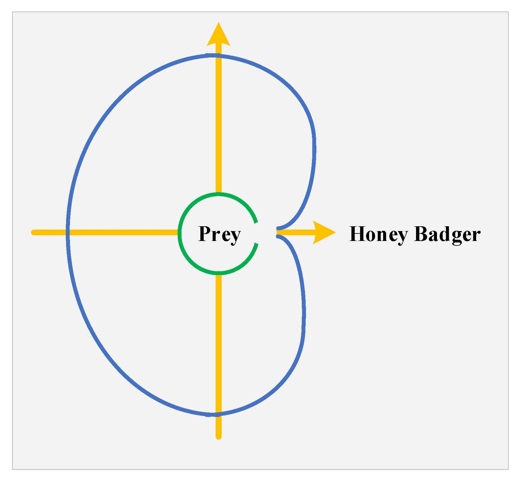
3.1. Overview of the HBA

An algorithm called the honey badger algorithm (HBA) was developed to mimic the way honey badgers forage [30]. The badger either searches for honey by sniffing and digging for it or by following a honeyguide bird. The drilling mode is the first, and the honey mode is the second. In the first scenario, it makes an approximation of the prey’s location using its smell sense. Once it reaches its destination, it circles the target to determine the optimal digging spot to capture it. Second, the beehives are independently located by the honey badger owing to the honeyguide bird’s map.

As previously mentioned, we break down the HBA into two steps: the “drilling phase” and the “honey phase”. This section presents the formula for the HBA algorithm. Theoretically, the HBA method qualifies as an overall optimization algorithm because it comprises discovery and exploitation phases. The HBA algorithm follows the steps listed below.

3.1.1. First Step: Initial Setting

Utilizing the following fundamental equation, the initial location of honey badgers is calculated [30]:

$$X_i={lb}_i+r_1\times \left({ub}_i-{lb}_i\right)$$

(26)

The random number, $r_1$, ranges from 0 to 1. The quantities lb and ub, respectively, represent the lower and upper boundaries of the search area, while $X_i$, the location of the honey badger, indicates a potential answer within the population size of N.

3.1.2. Second Step: Definition of Intensity

The honey badger’s intensity is determined by the prey’s focus and the distance between them. $I_i$ is a measure of how strongly a prey smells. The equation further down represents the opposite square law, which states that a strong scent leads to swift movement and vice versa [30].

$$\begin{gathered} I_i=r_2\times S/4\pi d_i^2 \\ S={\left(X_i-X_{i+1}\right)}^2 \\ {d}_i=x_{Prey}-x_i \end{gathered}$$

(27)

where S denotes the focus power source power (prey location) and d_i represents the distance between the prey and the ith badger.

3.1.3. Third Step: Updating the Density Coefficient

To provide an effortless move from exploring to exploitation, the density parameter (α) controls time-dependent unpredictability. The following expression is used for modifying the reduction factor, which reduces with each iteration, thereby lowering randomness over time [30].

$$\alpha =C\times exp\left(-t/t_{max}\right)$$

(28)

3.1.4. Fourth Step: Escape from the Local Optimum

In order to depart from local optimal regions, the subsequent three actions are implemented. In order to capitalize on the high likelihood that actors will accurately scan the search space in this scenario, the suggested method uses the F indicator.

3.1.5. Fifth Step: Update the Representative’s Position

As mentioned earlier, the procedure for upgrading the HBA location (x_new) is split into the “honey phase” and the “drilling phase.”

• Drilling phase

Throughout the drilling stage, the honey badger displays a cardioid-like motion, as illustrated in Figure 1. The motion of the cardioid may be approximated as follows [30]:

$$x_{new}=x_{prey}+F\times \beta \times I\times x_{prey}+F\times r_3\times \alpha \times d_i\times \left|\mathit{cos}(2\pi r_4)\right|\times \left[1-\mathit{cos}(2\pi r_5)\right]$$

(29)

where β is the finest location, the best position so far discovered, or the most advantageous location on Earth; $\beta \ge 1$ (usually set to six) denotes the honey badger’s capacity to obtain food; and d_i represents the space between the honey badger and its victim. Three separate integers ranging from zero to one are denoted by r₃, r₄, and r₅. The flag F modifies the search direction, which is determined by [30]

$$F=\left\{\begin{array}{c}1, \mathrm{i}\mathrm{f}{ r}_6\le 0.5\\ -1, \mathrm{e}\mathrm{l}\mathrm{s}\mathrm{e}\end{array}\right.$$

(30)

In the drilling stage, honey badgers are significantly influenced by the X_prey prey’s odor intensity, I; the distance they are from the prey, d_i; and the time-dependent search impact element, α. A badger may also experience any disruption during the drilling process that enables it to choose a hunting location that is significantly more advantageous (see Figure 1).

• Honey phase

One way to replicate the scenario where a honey badger follows a honeyguide bird to the hive is via [30]:

$$x_{new}=x_{prey}+F\times r_7\times \alpha \times d_i$$

(31)

where x_new refers to the honey badger’s relocated spot, while x_prey is the location of the prey; α and F are calculated using Equations (28) and (30), respectively. According to the distance data, a honey badger will search close to the location of the prey that has already been located. In this situation, the searching process is influenced by changing search behavior (α). A honey badger could also contract the F disease.

3.2. Overview of the Improved HBA (IHBA)

To accelerate the pace of convergence and the power of exploration and search in the badger algorithm, α decreases exponentially; changing it will change the power of discovery in this algorithm. In the original mode, the vector’s changes are nearly linear from the first iteration to the final iteration. However, the proposed method alters the vector’s value exponentially, following the chaotic sequence curve [31]. The value drops off faster as the number of repeats rises. This factor increases as the badgers get closer to the honey; their speed does not decrease linearly, but exponentially. Figure 2 displays the vector’s variation in two linear and exponential modes. Additionally, we calculate this vector using the following relation:

$$\begin{array}{l}W=rand(-2,2)\times [\sin ((\pi /2)\times (t/t_{\max }))+\cos ((\pi /2)\times (t/t_{\max }))-1]\\ Z=(2\times r_7+1)\times (1-t/t_{\max })+W\\ \alpha =C\times \exp (-t/t_{\max })\times Z\end{array}$$

(32)

Prominent Features of the IHBA are presented as follows:

• The search phases in the HBA can adapt based on the problem’s complexity. For example, in IHBA, the vector changes are made exponentially rather than linearly, following a chaotic sequence. This leads to faster convergence as the search process progresses, which is particularly useful for difficult optimization tasks.
• The enhanced version of HBA, IHBA, includes features like chaotic sequences and fuzzy decision-making. These features further improve the algorithm’s ability to handle complex optimization problems by enhancing the exploration and decision-making capabilities.

3.3. Multi-Objective Optimization Approach

Planners may have to choose the best option from a set of viable alternatives after determining which ones are Pareto optimal. The utilization of fuzzy decision-making, using a membership function, aims to achieve this crucial objective [28,32]. This will allow for the recording of additional variable values. Figure 3 depicts the optimization issue and the fuzzy decision function. The formula below delineates the membership function of the ith objective function for the optimized kth Pareto optimum solutions.

$${\xi }_i^k=\left\{\begin{array}{cc}1& f_i\le f_i^{min}\hfill \\ {\displaystyle \frac{f_i^{max}-f_i}{f_i^{max}-f_i^{min}}}& f_i^{min}\le f_i\le f_i^{max}\hfill \\ 0& f_i\ge f_i^{max}\hfill \end{array}\right.$$

(33)

where $f_i^{max}$ and $f_i^{min}$ are the upper and lower values of the ith function, corresponding to the non-dominated solutions, respectively. The ${\xi }_i^k$ value ranges from 0 to 1; ${\xi }_i^k=0$ means the solution indices are the sum of incompatibilities, while ${\xi }_i^k=1$ means full ability [28,32]. Here is how each of the k Pareto solutions has their normalized membership function calculated:

$${\xi }^k={\displaystyle \frac{\sum _{i=1}^m{\xi }_i^k}{\sum _{k=1}^n\sum _{i=1}^m{\xi }_i^k}}$$

(34)

where m is the number of the target function and n is the solution number that is not dominated.

Therefore, the compromised solution is calculated by

$$\mathit{max}\left\{{\xi }^k\left(X\right)\right\}$$

(35)

The best compromise is to use the membership function’s highest amount. In this research, cost of operation and emission—two conflicting functions—are simultaneously minimized using fuzzy methods.

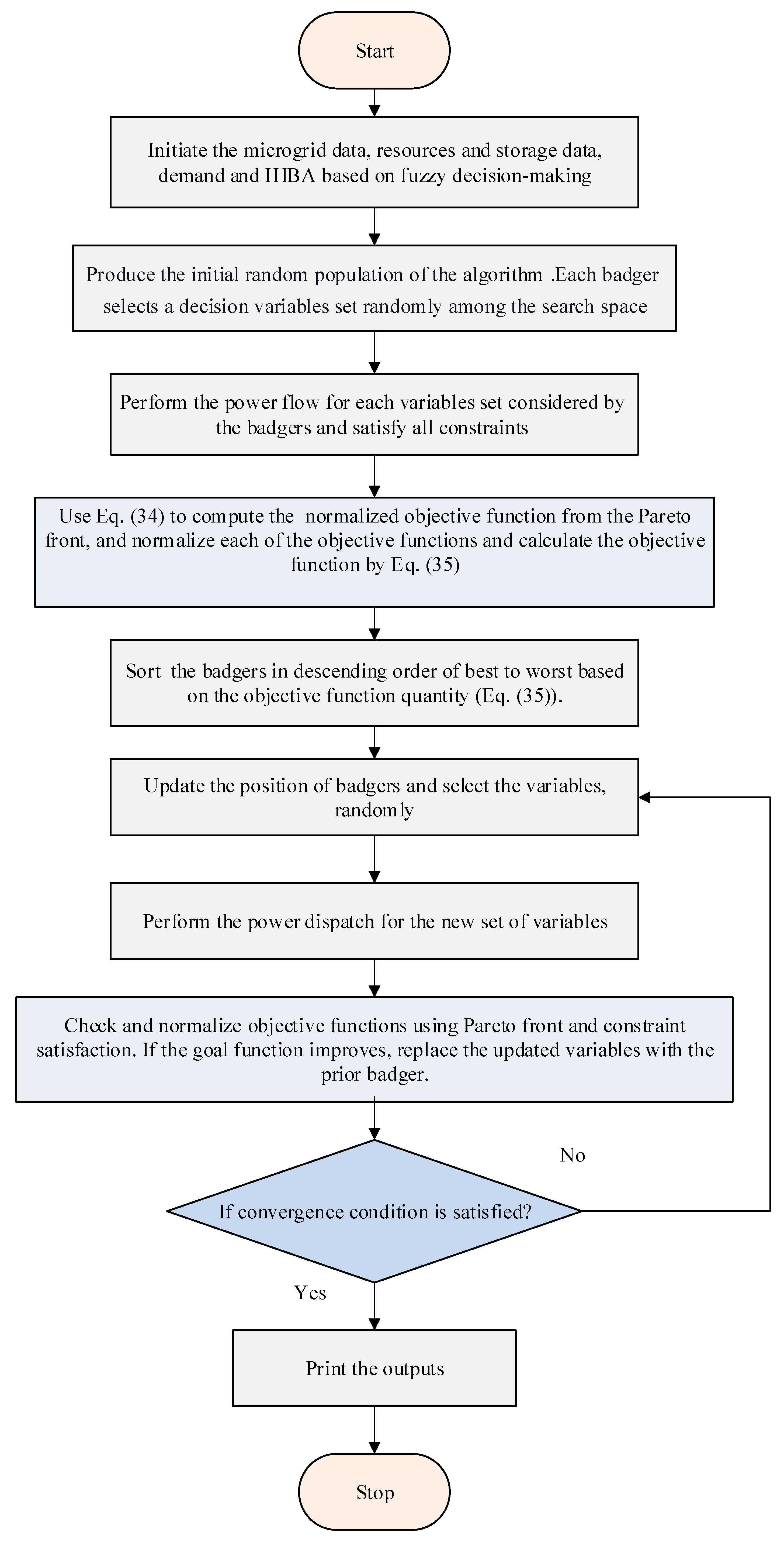
3.4. Implementation of the Fuzzy Multi-Objective IHBA

This section outlines the implementation steps of the fuzzy multi-objective IHBA to solve the problem.

Step 1: The optimization program begins by using the technical data of the microgrid (MG), including information on energy resources, load, market prices, and data related to the operation and emission costs of energy sources over a 24 h period.

Step 2: A set of variables within the permissible range is randomly determined for the algorithm’s population. These variables represent the size of energy and storage resources.

Step 3: The objective function value is calculated for each set of random variables selected in Step 2 that meets the operational constraints and energy resource requirements.

Step 4: Non-dominated solutions are identified from the set of solutions obtained in Step 3.

Step 5: The non-dominated solutions are separated from the other solutions and stored in an archive.

Step 6: The optimal honey badger is identified from the archive created in Step 5.

Step 7: The honey badger population and the positions of individual members are updated.

Step 8: The optimal honey badger with a non-dominated solution is added to the archive.

Step 9: Dominated solutions are removed from the archive, and additional members are also eliminated in proportion to the total number of archived members.

Step 10: The convergence criterion of the IHBA is assessed, which involves executing the maximum number of algorithm iterations. If convergence is achieved, the algorithm proceeds to Step 11; if not, it returns to Step 7.

Step 11: The final solution is determined using the fuzzy decision-making method from the final set of solutions.

The suggested approach is illustrated in Figure 4 by a flow diagram that uses fuzzy decision-making and the IHBA.

4. Results and Discussion

4.1. MG Data

The schematic of the MG connected to the power grid is depicted in Figure 5 [7]. Various kinds of DGs, including gas MTs, proton exchange membrane fuel cells (PEM-FCs), wind turbines, solar systems, and lithium-ion (Li-ion) battery storage technology, are included in the MG. All of these sources are deemed to generate active power having a power factor of unity. As a result of decisions made by the MG operator, a power exchange bridge connects the grid and MG for intraday trading in electricity. The main residential area, manufacturing feeders supplying a small workshop, and a feeder with light business users make up the MG’s load demand on an average day, resulting in a total energy consumption of 1695 kWh. The production limits and the participation rates of DGs in the MG are displayed in

Table 1. Power limits and participation costs of production units, storage devices, and emission coefficients [7].

Type	Min Power (kW)	Max Power (kW)	a (EURct/kW h2)	b (EURct/kW h)	c (EURct/h)	CO2 (kg/kWh)	SO2 (kg/kWh)	NOx (kg/kWh)
MT	6	30	0	0.457	0	720	0.0036	0.1
PV	0	25	0	2.584	0	0	0	0
FC	3	30	0	0.294	0	460	0.003	0.0075
WT	0	15	0	1.073	0	0	0	0
Battery	−30	30	0	0.380	0	10	0.0002	0.001
Grid	−30	30	0	-	0	950	0.5	2.1

. Figure 6 and Figure 7 show the anticipated data for the wind turbine, solar cell, load demand, and cost of purchasing and selling to the grid derived from Ref. [7].

4.2. Evaluating the IHBO’s Performance on the Benchmark Test Functions

This part uses nine well-known and frequently used classical test functions [33] to more accurately evaluate the performance of the IHBA algorithm. We select these functions to ensure they contain a large number of local points and, occasionally, even flat surfaces. If the algorithm can identify the best solutions for these functions, it is practically reliable.

Table 2. Classical test functions [33].

Function	Dim	Type	Range	fmin
$f_1\left(x\right)={\displaystyle \sum _{i=1}^n{x}_i^2}$	30	U	[−100,100]	0
$f_2\left(x\right)={\displaystyle \sum _{i=1}^n\left|x_i\right|}+{\displaystyle \prod _{i=1}^n\left|x_i\right|}$	30	U	[−10,10]	0
$f_3\left(x\right)={\displaystyle \sum _{i=1}^n{\left({\displaystyle \sum _{j-1}^i{x}_j}\right)}^2}$	30	U	[−100,100]	0
$\begin{array}{cc}{f}_4\left(x\right)={\max }_i\left\{\left|x_1\right|\right\}& ,1\le i\le n\end{array}$	30	U	[−100,100]	0
$f_5\left(x\right)={\displaystyle \sum _{i=1}^n\left[x_i^2-10\cos \left(2\pi x_1\right)+10\right]}$	30	M	[−5.12,5.12]	0
$f_6\left(x\right)={\displaystyle \frac{1}{4000}}{\displaystyle \sum _{i=1}^n{x}_i^2-{\displaystyle \prod _{i=1}^n\cos \left(\frac{x_i}{\sqrt{i}}\right)}}$	30	M	[−600,600]	0
$f_7\left(x\right)=-20\exp \left(-0.2\sqrt{{\displaystyle \frac{1}{n}}{\displaystyle \sum _{i=1}^n{x}_i^2}}\right)-\exp \left({\displaystyle \frac{1}{n}}{\displaystyle \sum _{i=1}^n\cos \left(2\pi x_i\right)}\right)+20+e$	30	M	[−32,32]	0
$f_8\left(x\right)={\displaystyle \sum _{i=1}^{11}\left[a_i-\frac{x_1\left(b_i^2+b_i{x}_2\right)}{b_i^2+b_i{x}_3+x_4}\right]}$	4	F	[−5,5]	0.003
$f_9\left(x\right)=-{{\displaystyle \sum _{i=1}^7\left[\left(X-a_i\right){\left(X-a_i\right)}^T+c_i\right]}}^{-1}$	4	F	[0,10]	−10

provides a list of the selected functions for evaluating the suggested algorithm. We specify these functions as unimodal functions (U), multimodal functions (M), and multimodal criterion functions with fixed dimensions (F). The IHBA algorithm is compared with the HBA and PSO algorithms.

Table 3. Optimization results on the test functions.

Functions	Quantity	PSO	HBA	IHBA
F1	Best	7.8077 × 10−8	3.0019 × 10−153	9.7372 × 10−223
	Mean	1.5307 × 10−6	6.322 × 10−147	6.2472 × 10−219
	STD	1.7177 × 10−6	2.0911 × 10−146	0
	Rank	3	2	1
F2	Best	0.00019619	1.941 × 10−81	1.7628 × 10−113
	Mean	0.0022842	2.4113 × 10−78	5.8859 × 10−111
	STD	0.0038183	3.2957 × 10−78	8.9739 × 10−111
	Rank	3	2	1
F3	Best	3.7395	1.3108 × 10−116	5.7235 × 10−214
	Mean	8.1127	7.1951 × 10−108	4.6432 × 10−209
	STD	2.7794	2.8384 × 10−107	0
	Rank	3	2	1
F4	Best	0.18804	1.3434 × 10−65	1.9347 × 10−109
	Mean	0.28315	6.4748 × 10−62	6.5422 × 10−107
	STD	0.074822	1.5819 × 10−61	1.877 × 10−106
	Rank	3	2	1
F5	Best	0.055889	9.7363 × 10−6	3.4035 × 10−6
	Mean	0.097544	0.00032382	0.00023109
	STD	0.029638	0.00043249	0.00020734
	Rank	2	1	1
F6	Best	22.2673	0	0
	Mean	42.5727	0	0
	STD	13.3025	0	0
	Rank	2	1	1
F7	Best	7.9936 × 10−15	8.8818 × 10−16	8.8818 × 10−16
	Mean	2.4993 × 10−13	8.8818 × 10−16	8.8818 × 10−16
	STD	3.0874 × 10−13	0	0
	Rank	2	1	1
F8	Best	2.436	0	0
	Mean	6.9443	0	0
	STD	2.7788	0	0
	Rank	2	1	1
F9	Best	0.00030751	0.00030749	0.00030749
	Mean	0.00056656	0.005241	0.0032009
	STD	0.0002199	0.0088553	0.0072998
	Rank	3	2	1

of the appendix presents the optimization results. This table specifies the best value, mean, and standard deviation for 30 executions, 200 repetitions, and a population of 30. Figure 8 also displays the convergence curve of three algorithms for test functions. The shape and results indicate that the differential component of the suggested algorithm has accelerated the convergence of the IHBA algorithm, leading to a superior global optimal solution. The IHBA algorithm has shown its competence in dealing with local minima.

4.3. Simulation Scenarios

Findings from optimizing an MG’s EMS with the suggested algorithm are detailed here. We have run simulations in multiple scenarios to thoroughly test the proposed strategy. The three algorithms—IHBA, HBA, and PSO—are thought of as identical when they use 100 iterations and 50 populations. The following are the possible outcomes:

• First scenario: MG energy management and scheduling with operation cost reduction
• Second scenario: MG energy management and scheduling with emission reduction
• Third scenario: MG energy management and scheduling with operation and emission cost reduction based on fuzzy multi-objective function
• Fourth scenario: MG energy management and scheduling with operation and emission cost reduction based on fuzzy multi-objective function incorporating battery aging.

4.3.1. Results of First Scenario

In this section, energy management and scheduling using predicted data, with the objective of reducing operating costs, are investigated and simulated. Figure 9 presents the convergence curves of three algorithms. These curves indicate that the IHBA algorithm exhibits high consistency and good accuracy in the final solution.

Table 4. The best results obtained in the first scenario with the objective function of operating cost reduction.

Time (h)	Load	Power (kW)						Cost (EURct/h)	Emission (kg/h)
		PV	WT	MT	FC	Battery	Utility
1	52	0	1.785	6	30	−15.785	30	14.379	46.5411
2	50	0	1.785	6	30	−17.785	30	12.419	46.5211
3	50	0	1.785	6	30	−17.785	30	10.919	46.5211
4	51	0	1.785	6	30	−16.785	30	10.699	46.5311
5	56	0	1.785	6	30	−11.785	30	12.599	46.5811
6	63	0	0.915	6	30	−3.9150	30	17.0561	46.6598
7	70	0	1.785	6	30	2.215	30	21.219	46.7211
8	75	0.2	1.305	6	30	15.3714	22.1236	27.7272	28.8545
9	76	3.75	1.785	30	30	30	−19.535	16.2328	17.0944
10	80	7.525	3.09	30	30	30	−20.615	−25.7698	16.0656
11	78	10.45	8.775	28.775	30	30	−30.000	−50.2115	6.2434
12	74	11.95	10.41	21.64	30	30	−30.000	−47.8418	1.1062
13	72	23.9	3.915	14.185	30	30	−30.000	47.6609	−4.2630
14	72	21.05	2.37	18.58	30	30	−30.000	−34.3527	−1.0981
15	76	7.875	1.785	30	30	30	−23.660	8.8743	13.1649
16	80	4.225	1.305	30	30	30	−15.530	15.9639	20.9096
17	85	0.55	1.785	30	30	30	−7.3350	32.8655	28.7161
18	88	0	1.785	6	30	30	20.215	33.1655	37.6778
19	90	0	1.302	6	30	22.698	30	32.0843	46.9259
20	87	0	1.785	6	30	30	19.215	33.1398	36.7252
21	78	0	1.3005	30	30	30	−13.300	19.7639	23.0334
22	71	0	1.3005	30	30	30	−20.300	24.3632	16.3652
23	65	0	0.915	6	30	−1.9150	30	20.8161	46.6798
24	56	0	0.615	6	30	−10.615	30	15.9882	46.5928
						Total (per/day):		269.7599	706.87

shows the best results achieved for the cost objective function using the recommended IHBA. Additionally, Figure 10 displays the production power of each source. Analyzing the results reveals that all equality and inequality constraints are met.

Although the involvement of the respective units is lower during these periods compared with other times in the investigated period, the numerical results in Table 4 demonstrate that a significant portion of the demand is provided by the fuel cell and the grid. Market prices are much higher between the hours of 9:00 and 17:00, as well as 21:00 and 22:00. During these times, the microturbine output power increases, and any excess energy is fed from the MG to the grid. The battery-charging procedure is carried out between the hours of 1:00 and 6:00 and 11:00 and 24:00, when market prices are at their lowest.

Table 5. Comparison of the outcomes of different methods in the first scenario.

Objective	Method	Best Solution
Cost (EURct)	GA [7]	277.7444
	PSO [7]	277.3237
	FSAPSO [7]	276.7867
	CPSO-T [7]	275.0455
	CPSO-L [7]	274.7438
	AMPSO-T [7]	274.5507
	AMPSO-L [7]	274.4317
	GSA [7]	275.5369
	SGSA [7]	269.76
	HBA	269.76
	IHBA	269.7599

compares the obtained results of the proposed IHBA method described in this study with those of several different algorithms presented in other sources, taking into account the cost objective function. Table 5 shows that the proposed approach works better than a number of other ways to solve problems with energy management and use. This is because the results produced by IHBA are either better than or about the same as those produced by other methods. This highlights its capacity to provide higher-quality solutions.

4.3.2. Results of Second Scenario

This section investigates and simulates energy planning and management in a deterministic manner using predicted data, taking into account the objective function of pollution reduction. Due to the fact that a part of the load supply power is supplied by the microturbine and the grid, the pollution from these two sources of power supply is high. In order to reduce the pollution in this section, planning has been done considering the objective function of pollution only. Figure 11 shows the convergence curve of three algorithms. These curves indicate that the IHBA algorithm, similar to the first scenario, demonstrates robust convergence and a lower value for the objective function in comparison with either of the two algorithms.

Table 6. The best results obtained in the second scenario with the objective function of emission reduction.

Time (h)	Load	Power (kW)						Cost (EURct/h)	Emission (kg/h)
		MT	FC	PV	WT	Battery	Utility
1	52	20.215	30	0	1.785	30	−30	24.47356	0.079245
2	50	18.215	30	0	1.785	30	−30	24.75956	−1.36096
3	50	18.215	30	0	1.785	30	−30	26.25956	−1.36096
4	51	19.215	30	0	1.785	30	−30	27.31656	−0.64086
5	56	24.215	30	0	1.785	30	−30	29.60156	2.95966
6	63	30	30	0	0.915	30	−27.915	29.3288	9.11163
7	70	30	30	0	1.785	30	−21.785	30.83476	14.95107
8	75	30	30	0.2	1.305	30	−16.505	29.57517	19.9808
9	76	30	30	3.75	1.785	30	−19.535	16.23281	17.09442
10	80	30	30	7.525	3.09	30	−20.615	−25.7698	16.06561
11	78	28.775	30	10.45	8.775	30	−30	−50.2115	6.243332
12	74	21.64	30	11.95	10.41	30	−30	−47.8418	1.105393
13	72	14.185	30	23.9	3.915	30	−30	47.66094	−4.26298
14	72	18.58	30	21.05	2.37	30	−30	−34.3527	−1.09812
15	76	30	30	7.875	1.785	30	−23.66	8.874305	13.16494
16	80	30	30	4.225	1.305	30	−15.53	15.96417	20.90958
17	85	30	30	0.55	1.785	30	−7.335	32.86551	28.71614
18	88	30	30	0	1.785	30	−3.785	34.29346	32.09787
19	90	30	30	0	1.302	30	−1.302	34.87135	34.46317
20	87	30	30	0	1.785	30	−4.785	33.78776	31.14527
21	78	30	30	0	1.3005	30	−13.300	19.76385	23.0334
22	71	30	30	0	1.3005	30	−20.300	24.36317	16.3652
23	65	30	30	0	0.915	30	−25.915	27.1373	11.01683
24	56	25.385	30	0	0.615	30	−30	24.68084	3.802181
						Total (per/day):		384.4691	293.5819

and

Table 7. The best results obtained for the third scenario with the multi-objective function.

Time (h)	Load	Power (kW)						Cost (EURct/h)	Emission (kg/h)
		MT	FC	PV	WT	Battery	Utility
1	52	6	30	0	1.785	30	−15.785	21.24676	3.384182
2	50	6	30	0	1.785	30	−17.785	21.49816	1.478982
3	50	6	3	0	1.785	30	9.215	13.24101	34.37081
4	51	6	3	0	1.785	30	10.215	13.021	34.38082
5	56	6	3	0	1.785	30	15.215	14.92101	34.43082
6	63	6	30	0	0.915	30	−3.915	23.1608	14.69154
7	70	6	30	0	1.785	30	2.215	25.38676	20.53098
8	75	6	30	0.2	1.305	30	7.495	27.72717	25.56071
9	76	30	30	3.75	1.785	30	−19.535	16.23281	17.09442
10	80	30	30	7.525	3.09	30	−20.615	−25.7698	16.06561
11	78	28.77501	30	10.45	8.775	30	−30	−50.2033	6.266408
12	74	21.64001	30	11.95	10.41	30	−30	−47.8418	1.10539
13	72	14.185	30	23.9	3.915	30	−30	47.66094	−4.26298
14	72	18.58002	30	21.05	2.37	30	−30	−34.3504	−1.08075
15	76	30	30	7.875	1.785	30	−23.66	8.874305	13.16494
16	80	30	30	4.225	1.305	30	−15.53	15.96417	20.90958
17	85	30	30	0.55	1.785	30	−7.335	32.86551	28.71614
18	88	30	30	0	1.785	30	−3.785	34.29346	32.09787
19	90	6	30	0	1.302	30	22.698	32.30335	40.04309
20	87	30	30	0	1.785	30	−4.785	33.78776	31.14527
21	78	30	30	0	1.3005	30	−13.300	19.76385	23.0334
22	71	30	30	0	1.3005	30	−20.3	24.36317	16.3652
23	65	6	30	0	0.915	30	−1.915	23.3693	16.59674
24	56	6	30	0	0.615	30	−10.615	20.862	8.309124
						Total (per/day):		312.3778	434.3983

display the optimal outcomes of the IHBA method for the emission objective function. Figure 12 also displays the production power of each source. The analysis of the findings reveals that all constraints are satisfied.

Table 6’s results indicate that during 24 h periods, the fuel cell and battery supply a significant portion of the demand, as their participation is lower than in other cases during the studied period. The network has been selling more power due to the higher pollution levels. By optimizing the pollution, its amount has decreased from 706 kg per day to 293 kg per day compared with the previous state, but the operating cost has increased.

4.3.3. Results of Third Scenario

Reducing pollution raises costs, and lowering costs raises pollution. Because these two effects are opposite, energy planning and management with predicted data is studied and simulated, with the goals of lowering costs and pollution as the main factors. We utilize the Pareto front method to identify the optimal solution set. Then, by utilizing fuzzy decision-making, we determine the balanced solution between these two objective functions from the optimal solution set. Figure 13 displays both the fuzzy decision solution and the Pareto curve of the optimal solution set. According to this form, the proposed algorithm has been able to archive a set of better answers. Table 7 displays the optimal outcomes from the fuzzy decision-making stage, utilizing the proposed IHBA method for both the cost and pollution objective functions. Figure 14 also displays the production power of each source.

According to the results of Table 7, both pollution and production costs are lower in the simulation time of 24 h than in the second case. Additionally, the fuel cell and battery supply a significant portion of the demand, with the network stepping in during higher-cost hours.

In

Table 8. Comparison of the outcomes of different methods in the third scenario.

Method	Cost (EURct/h)	Emission (kg/h)
NSGA-II	314.1799	435.7832
MOPSO	314.8394	436.362
MOHBA	314.2022	436.2702
MOIHBA	312.3778	434.3983

, the performance of the multi-objective IHBA (MOIHBA) is compared with NSGA-II, MOPSO, and multi-objective HBA (MOHBA). The obtained results demonstrate the superior performance of the MOIHBA compared with other algorithms with lower operating and emission costs.

4.3.4. Results of Fourth Scenario

Since the lifespan of batteries depends on the number of charges and discharges, the use of these resources increases the exploitation and other costs related to repair and maintenance. This section examines the impact of battery aging as a limitation and the cost associated with aging in the goal functions. Figure 15 shows the Pareto curve for the fourth scenario with the IHBA algorithm. According to this curve, which represents the set of optimal solutions based on

Table 9. The best results obtained for the fourth scenario with the multi-objective function.

Time (h)	Load	Power (kW)						Cost (EURct/h)	Emission (kg/h)
		MT	FC	PV	WT	Battery	Utility
1	52	6	30	0	1.785	30	−15.785	13.88786	3.384182
2	50	6	30	0	1.785	30	−17.785	13.81646	1.478982
3	50	6	12.215	0	1.785	0	30	8.498414	38.51765
4	51	6	13.21498	0	1.785	0	30	8.756708	38.97765
5	56	6	18.21499	0	1.785	0	30	10.22671	41.27771
6	63	6	30	0	0.915	30	−3.915	12.7268	14.69154
7	70	6	30	0	1.785	30	2.215	13.88786	20.53098
8	75	6	30	0.2	1.305	30	7.495	14.05097	25.56071
9	76	30	30	3.75	1.785	30	−19.535	38.23781	17.09442
10	80	30	30	7.525	3.09	30	−20.615	60.50967	16.06561
11	78	28.775	30	10.45	8.775	30	−30	97.45955	6.243332
12	74	21.64	30	11.95	10.41	30	−30	106.9392	1.105393
13	72	14.185	30	23.9	3.915	30	−30	96.21544	−4.26298
14	72	18.57988	30	21.05	2.37	30	−29.9999	91.72622	−1.0981
15	76	30	30	7.875	1.785	30	−23.66	51.35681	13.16494
16	80	30	30	4.225	1.305	30	−15.53	38.99792	20.90958
17	85	30	30	0.55	1.785	30	−7.335	27.14651	28.71614
18	88	30	30	0	1.785	30	−3.785	25.17716	32.09787
19	90	6	30	0	1.302	30	22.698	13.41475	40.04309
20	87	30	30	0	1.785	30	−4.785	25.21286	31.14527
21	78	30	30	0	1.3005	30	−13.3005	25.44702	23.0334
22	71	30	30	0	1.3005	30	−20.3005	24.62771	16.3652
23	65	6	30	0	0.915	30	−1.915	12.8183	16.59674
24	56	6	30	0	0.615	30	−10.615	12.3818	8.309124
						Total (per/day):		335.6221	449.9484

, the operating cost in the lowest value is equal to 291.78, indicating an increase compared with the first scenario. This 7.6% increase is due to the cost of depreciation. The reduction in battery usage in MG energy management accounts for this increase. Figure 16 displays the fuzzy decision-making results from the set of Pareto solutions. Table 9 also provides information on the power of each source. According to the table, the battery’s injected power is zero at 03:00–05:00 h. The cost of operation and pollution despite battery aging is equal to 335.622 and 449.94, respectively, which has increased compared with a scenario without battery aging.

5. Conclusions

The aim of this study was to lower operational and emission costs by applying the MOIHBA, a new optimization technique based on fuzzy decision-making, for energy management in an MG. The approach involved assessing decision variables such as the capacity of multi-energy units and storage resources to determine the optimal value for each hour. It also took into account operational and device constraints as well as two objective functions. This method has the potential to help operators make more informed decisions about day-ahead resource production in MG energy management. The predicted data were applied to the sample MG in various scenarios to determine the results of the recommended approach. The results are as follows:

• In the first scenario, the single-objective IHBA was utilized for energy management and scheduling of the MG, aiming to reduce operating costs. The results demonstrated that the IHBA delivers high consistency and accuracy, which are crucial for achieving the most optimal solution. Furthermore, this method outperforms many other approaches by achieving lower costs. The findings also indicated that the outcomes from the IHBA are superior to those from traditional HBA and PSO methods as well as from previous studies. The optimization process led to a decrease in operating costs compared with the baseline state.
• In the second scenario, the single-objective IHBA was used for planning and energy management of the MG with a focus on minimizing emission costs. The results demonstrated that, like in the first scenario, the IHBA achieved a lower objective function and exhibited superior convergence compared with traditional HBA and PSO algorithms. This scenario successfully minimized emission costs while adhering to the constraints of the optimization problem. Although the optimization process led to a reduction in emission costs compared with the initial scenario, it also resulted in an increase in operating costs.
• The third scenario was implemented using the suggested multi-objective method by striking a compromise between different objectives, as evidenced by the results of the third scenario’s implementation with the multi-objective optimization of the MG, which considers the objectives of minimizing emissions and operation costs. The results showed that the emission cost decreased more than the operating cost, despite the fact that the multi-objective optimization increased the operating cost in comparison with the first scenario.
• The assessment of battery aging effects on MG optimization in the fourth scenario showed that the problem’s objective function experienced a rise in production and emission costs due to the battery’s power injection constraints. Specifically, these costs increased by 7.44% and 3.58%, respectively, compared with scenarios without battery aging.
• The IHBA shows superior performance compared with two conventional algorithms, HBA and PSO, by exhibiting more favorable and rapid convergence, overcoming local minima, and effectively balancing exploration and exploitation. This is evident from the results of applying the new, improved optimization method, which is based on chaotic sequences, to the EMS problem and the standard test functions. The IHBA’s ability to navigate complex problem spaces more efficiently and to consistently achieve optimal solutions underscores its potential for enhancing energy management systems and addressing challenges in optimization tasks.
• Future research is recommended to focus on robust optimization and energy management for multi-energy MGs that incorporate hydrogen storage, incorporating machine learning and RBF networks to forecast the renewable and load data. This involves minimizing operational and emission costs through the application of a novel optimization algorithm. By leveraging advanced techniques, the researchers aim to enhance the efficiency and sustainability of MG systems, ensuring optimal performance while reducing environmental impact. The development of such algorithms will address the complexities associated with integrating hydrogen storage, ultimately leading to more effective and cost-efficient energy management strategies.

References

1. Suresh, V.; Janik, P.; Jasinski, M.; Guerrero, J.M.; Leonowicz, Z. Microgrid Energy Management Using Metaheuristic Optimization Algorithms. Appl. Soft Comput. 2023, 134, 109981. [Google Scholar] [CrossRef]
2. Aghajani, G.R.; Shayanfar, H.A.; Shayeghi, H. Demand side management in a smart micro-grid in the presence of renewable generation and demand response. Energy 2017, 126, 622–637. [Google Scholar] [CrossRef]
3. Karimi, H.; Jadid, S.; Hasanzadeh, S. Optimal-Sustainable Multi-Energy Management of Microgrid Systems Considering Integration of Renewable Energy Resources: A Multi-Layer Four-Objective Optimization. Sustain. Prod. Consum. 2023, 36, 126–138. [Google Scholar] [CrossRef]
4. Sepehrzad, R.; Rahimi, M.K.; Al-Durra, A.; Allahbakhshi, M.; Moridi, A. Optimal Energy Management of Distributed Generation in Micro-Grid to Control the Voltage and Frequency Based on PSO-Adaptive Virtual Impedance Method. Electr. Power Syst. Res. 2022, 208, 107881. [Google Scholar] [CrossRef]
5. Sepehrzad, R.; Mahmoodi, A.; Ghalebi, S.Y.; Moridi, A.R.; Seifi, A.R. Intelligent Hierarchical Energy and Power Management to Control the Voltage and Frequency of Micro-Grids Based on Power Uncertainties and Communication Latency. Electr. Power Syst. Res. 2022, 202, 107567. [Google Scholar] [CrossRef]
6. Zhang, H.; Ma, Y.; Yuan, K.; Khayatnezhad, M.; Ghadimi, N. Efficient Design of Energy Microgrid Management System: A Promoted Remora Optimization Algorithm-Based Approach. Heliyon 2024, 10, e23394. [Google Scholar] [CrossRef]
7. Moghaddam, A.A.; Seifi, A.; Niknam, T.; Pahlavani, M.R.A. Multi-Objective Operation Management of a Renewable MG (Micro-Grid) with Back-up Micro-Turbine/Fuel Cell/Battery Hybrid Power Source. Energy 2011, 36, 6490–6507. [Google Scholar] [CrossRef]
8. Kumar, R.P.; Karthikeyan, G. A Multi-Objective Optimization Solution for Distributed Generation Energy Management in Microgrids with Hybrid Energy Sources and Battery Storage System. J. Energy Storage 2024, 75, 109702. [Google Scholar] [CrossRef]
9. Hai, T.; Zhou, J.; Khaki, M. Optimal Planning and Design of Integrated Energy Systems in a Microgrid Incorporating Electric Vehicles and Fuel Cell System. J. Power Sources 2023, 561, 232694. [Google Scholar] [CrossRef]
10. Dey, B.; Misra, S.; Marquez, F.P.G. Microgrid System Energy Management with Demand Response Program for Clean and Economical Operation. Appl. Energy 2023, 334, 120717. [Google Scholar] [CrossRef]
11. Alamir, N.; Kamel, S.; Megahed, T.F.; Hori, M.; Abdelkader, S.M. Developing Hybrid Demand Response Technique for Energy Management in Microgrid Based on Pelican Optimization Algorithm. Electr. Power Syst. Res. 2023, 214, 108905. [Google Scholar] [CrossRef]
12. Lu, Z.; Gao, Y.; Xu, C.; Li, Y. Configuration optimization of an off-grid multi-energy microgrid based on modified NSGA-II and order relation-TODIM considering uncertainties of renewable energy and load. J. Clean. Prod. 2023, 383, 135312. [Google Scholar] [CrossRef]
13. Parvin, M.; Yousefi, H.; Noorollahi, Y. Techno-economic optimization of a renewable micro grid using multi-objective particle swarm optimization algorithm. Energy Convers. Manag. 2023, 277, 116639. [Google Scholar] [CrossRef]
14. Ferahtia, S.; Rezk, H.; Abdelkareem, M.A.; Olabi, A.G. Optimal Techno-Economic Energy Management Strategy for Building’s Microgrids Based Bald Eagle Search Optimization Algorithm. Appl. Energy 2022, 306, 118069. [Google Scholar] [CrossRef]
15. Dey, B.; Raj, S.; Mahapatra, S.; Márquez, F.P.G. Optimal Scheduling of Distributed Energy Resources in Microgrid Systems Based on Electricity Market Pricing Strategies by a Novel Hybrid Optimization Technique. Int. J. Electr. Power Energy Syst. 2022, 134, 107419. [Google Scholar] [CrossRef]
16. Sun, S.; Wang, C.; Wang, Y.; Zhu, X.; Lu, H. Multi-Objective Optimization Dispatching of a Micro-Grid Considering Uncertainty in Wind Power Forecasting. Energy Rep. 2022, 8, 2859–2874. [Google Scholar] [CrossRef]
17. Eskandari, H.; Kiani, M.; Zadehbagheri, M.; Niknam, T. Optimal Scheduling of Storage Device, Renewable Resources and Hydrogen Storage in Combined Heat and Power Microgrids in the Presence Plug-in Hybrid Electric Vehicles and Their Charging Demand. J. Energy Storage 2022, 50, 104558. [Google Scholar] [CrossRef]
18. Xiaoluan, Z.; Farajian, H.; Xifeng, W.; Latifi, M.; Ohshima, K. Scheduling of Renewable Energy and Plug-in Hybrid Electric Vehicles Based Microgrid Using Hybrid Crow—Pattern Search Method. J. Energy Storage 2022, 47, 103605. [Google Scholar] [CrossRef]
19. Dey, B.; Márquez, F.P.G.; Panigrahi, P.K.; Bhattacharyya, B. A Novel Metaheuristic Approach to Scale the Economic Impact of Grid Participation on a Microgrid System. Sustain. Energy Technol. Assess. 2022, 53, 102417. [Google Scholar] [CrossRef]
20. Taghikhani, M.A.; Khamseh, J. Multi-Objective Optimal Energy Management of Storage System and Distributed Generations via Water Cycle Algorithm Concerning Renewable Resources Uncertainties and Pollution Reduction. J. Energy Storage 2022, 52, 104756. [Google Scholar] [CrossRef]
21. Liao, N.; Hu, Z.; Mrzljak, V.; Arabi Nowdeh, S. Stochastic Techno-Economic Optimization of Hybrid Energy System with Photovoltaic, Wind, and Hydrokinetic Resources Integrated with Electric and Thermal Storage Using Improved Fire Hawk Optimization. Sustainability 2024, 16, 6723. [Google Scholar] [CrossRef]
22. Nowdeh, S.A.; Naderipour, A.; Davoudkhani, I.F.; Guerrero, J.M. Stochastic optimization–based economic design for a hybrid sustainable system of wind turbine, combined heat, and power generation, and electric and thermal storages considering uncertainty: A case study of Espoo, Finland. Renew. Sustain. Energy Rev. 2023, 183, 113440. [Google Scholar] [CrossRef]
23. Sun, H.; Cui, X.; Latifi, H. Optimal management of microgrid energy by considering demand side management plan and maintenance cost with developed particle swarm algorithm. Electr. Power Syst. Res. 2024, 231, 110312. [Google Scholar] [CrossRef]
24. Habibi, S.; Effatnejad, R.; Hedayati, M.; Hajihosseini, P. Stochastic energy management of a microgrid incorporating two-point estimation method, mobile storage, and fuzzy multi-objective enhanced grey wolf optimizer. Sci. Rep. 2024, 14, 1667. [Google Scholar]
25. Upadhyay, S.; Ahmed, I.; Mihet-Popa, L. Energy Management System for an Industrial Microgrid Using Optimization Algorithms-Based Reinforcement Learning Technique. Energies 2024, 17, 3898. [Google Scholar] [CrossRef]
26. Adam, S.P.; Alexandropoulos, S.A.N.; Pardalos, P.M.; Vrahatis, M.N. No free lunch theorem: A review. In Approximation and Optimization: Algorithms, Complexity and Applications; Springer: Berlin/Heidelberg, Germany, 2019; pp. 57–82. [Google Scholar]
27. Schwenk, K.; Meisenbacher, S.; Briegel, B.; Harr, T.; Hagenmeyer, V.; Mikut, R. Integrating Battery Aging in the Optimization for Bidirectional Charging of Electric Vehicles. IEEE Trans. Smart Grid 2021, 12, 5135–5145. [Google Scholar] [CrossRef]
28. Aghajani, G.R.; Shayanfar, H.A.; Shayeghi, H. Presenting a Multi-Objective Generation Scheduling Model for Pricing Demand Response Rate in Micro-Grid Energy Management. Energy Convers. Manag. 2015, 106, 308–321. [Google Scholar] [CrossRef]
29. Yahiaoui, A.; Fodhil, F.; Benmansour, K.; Tadjine, M.; Cheggaga, N. Grey Wolf Optimizer for Optimal Design of Hybrid Renewable Energy System PV-Diesel Generator-Battery: Application to the Case of Djanet City of Algeria. Sol. Energy 2017, 158, 941–951. [Google Scholar] [CrossRef]
30. Hashim, F.A.; Houssein, E.H.; Hussain, K.; Mabrouk, M.S.; Al-Atabany, W. Honey Badger Algorithm: New Metaheuristic Algorithm for Solving Optimization Problems. Math. Comput. Simul. 2022, 192, 84–110. [Google Scholar] [CrossRef]
31. Mokeddem, D. A New Improved Salp Swarm Algorithm Using Logarithmic Spiral Mechanism Enhanced with Chaos for Global Optimization. Evol. Intell. 2021, 15, 1745–1775. [Google Scholar] [CrossRef]
32. Nowdeh, S.A.; Davoudkhani, I.F.; Moghaddam, M.J.H.; Najmi, E.S.; Abdelaziz, A.Y.; Ahmadi, A.; Razavi, S.E.; Gandoman, F.H. Fuzzy Multi-Objective Placement of Renewable Energy Sources in Distribution System with Objective of Loss Reduction and Reliability Improvement Using a Novel Hybrid Method. Appl. Soft Comput. 2019, 77, 761–779. [Google Scholar] [CrossRef]
33. Golalipour, K.; Nowdeh, S.A.; Akbari, E.; Hamidi, S.S.; Ghasemi, D.; Abdelaziz, A.Y.; Kotb, H.; Yousef, A. Snow Avalanches Algorithm (SAA): A New Optimization Algorithm for Engineering Applications. Alex. Eng. J. 2023, 83, 257–285. [Google Scholar] [CrossRef]
Figure 1. Excavation stage: blue plot is odor intensity; green circular line indicates prey position.
Energies 17 04373 g001
Figure 2. Variation in the α coefficient over the algorithm’s iterations.
Energies 17 04373 g002
Figure 3. Implementation of fuzzy decision-making to choose the best solution from the Pareto set.
Energies 17 04373 g003
Figure 4. The suggested IHBA fuzzy decision-making technique flowchart.
Energies 17 04373 g004
Figure 5. Schematic of the studied MG.
Energies 17 04373 g005
Figure 6. Profile of irradiance (yellow box) and wind speed (blue line) during a day [7].
Energies 17 04373 g006
Figure 7. Profile of forecasted demand and market price during a day [7].
Energies 17 04373 g007
Figure 8. Convergence curve of three algorithms for the classical test functions.
Energies 17 04373 g008aEnergies 17 04373 g008bEnergies 17 04373 g008c
Figure 9. Convergence curve of optimization algorithms for first scenario.
Energies 17 04373 g009
Figure 10. The best components size obtained in the first scenario using IHBA.
Energies 17 04373 g010
Figure 11. Convergent curve of optimization algorithms for the second scenario.
Energies 17 04373 g011
Figure 12. The best components size obtained in the second scenario using IHBA.
Energies 17 04373 g012
Figure 13. The Pareto solution set of different algorithms for the third scenario.
Energies 17 04373 g013
Figure 14. The best components size obtained in the third scenario using IHBA.
Energies 17 04373 g014
Figure 15. The Pareto solution set of different algorithms for the fourth scenario.
Energies 17 04373 g015
Figure 16. The best components size obtained in the fourth scenario using IHBA.
Energies 17 04373 g016