Carbon Price Forecasting Using Optimized Sliding Window Empirical Wavelet Transform and Gated Recurrent Unit Network to Mitigate Data Leakage

Abstract

Precise forecasts of carbon prices are crucial for reducing greenhouse gas emissions and promoting sustainable, low-carbon development. To mitigate noise interference in carbon price data, hybrid models integrating data decomposition techniques are commonly utilized. However, it has been observed that the improper utilization of data decomposition techniques can lead to data leakage, thereby invalidating the model’s practical applicability. This study introduces a leakage-free hybrid model for carbon price forecasting based on the sliding window empirical wavelet transform (SWEWT) algorithm and the gated recurrent unit (GRU) network. First, the carbon price data are sampled using a sliding window approach and then decomposed into more stable and regular subcomponents through the EWT algorithm. By exclusively employing the data from the end of the window as input, the proposed method can effectively mitigate the risk of data leakage. Subsequently, the input data are passed into a multi-layer GRU model to extract patterns and features from the carbon price data. Finally, the optimized hybrid model is obtained by iteratively optimizing the hyperparameters of the model using the tree-structured Parzen estimator (TPE) algorithm, and the final prediction results are generated by the model. When used to forecast the closing price of the Guangdong Carbon Emission Allowance (GDEA) for the last nine years, the proposed hybrid model achieves outstanding performance with an R² value of 0.969, significantly outperforming other structural variants. Furthermore, comparative experiments from various perspectives have validated the model’s structural rationality, practical applicability, and generalization capability, confirming that the proposed framework is a reliable choice for carbon price forecasting.

1. Introduction

In recent years, there has been a global consensus on the imperative to curtail carbon emissions to mitigate the impacts of global warming stemming from excessive greenhouse gas releases [1]. Institutionalized carbon trading schemes and carbon pricing policies are considered pivotal drivers in advancing emission reduction goals and facilitating the transition toward a low-carbon economy [2,3]. The carbon price, as the fundamental metric within the carbon market, not only mirrors the dynamics of carbon allowance supply and demand but also exerts a significant influence on the decisions of investors and regulators [4]. Precise forecasting of carbon prices is pivotal for steering investments toward carbon emission mitigation, bolstering the efficacy of emission reduction endeavors and providing a foundation for crafting policies directed at curbing carbon emissions [5,6]. However, in contrast to traditional financial markets, the carbon market is relatively young and characterized by an immature market system that is susceptible to external factors such as regulation and policies [7]. These external factors contribute to significant fluctuations in the carbon price, meaning that the market is characterized by nonlinearity, non-stationarity, and uncertainty [8], posing a great challenge for carbon price forecasting [9,10].

The significance of carbon prices has garnered extensive attention from scholars both domestically and internationally, leading to the development of numerous methods and models for carbon price forecasting. Traditional carbon price forecasting models, such as autoregressive integrated moving average (ARIMA) [11], support vector regression (SVR) [12], and random forest (RF) models [13], have demonstrated certain abilities in carbon price forecasting. However, these models rely heavily on high-quality data and consequently exhibit limited accuracy when confronted with highly volatile carbon price data [14], constraining their practical applicability. In recent years, deep learning models, such as long short-term memory (LSTM) [15], gated recurrent unit (GRU) [16], and other neural networks, have garnered attention for their ability to capture both long-term and short-term dependencies in time-series data. This capability has bestowed upon them an advantage over traditional models in regard to forecasting carbon prices. For example, Li et al. [17] applied LSTM to forecast carbon prices in Hubei and Guangdong and compared them with traditional models. The results indicate that, from the perspective of the root mean square error (RMSE), the LSTM achieves a performance improvement of 68.07% to 82.09% compared to SVR. Deep learning models are adept at capturing the intricate nonlinear dynamics of carbon prices, substantially improving the precision of predictive models. Nonetheless, challenges such as overfitting and entrapment in local optima can impede their consistent ability to yield accurate forecasts [18,19].

Given the inherent volatility and complexity of the carbon market, skepticism regarding the accuracy and reliability of single predictive models has been prevalent, whether employing traditional or deep learning approaches [20]. To enhance model performance, data decomposition techniques have been introduced into the field of carbon price forecasting, leading to the emergence of hybrid models [18,21]. For instance, Wu et al. [1] combined variational mode decomposition (VMD) with CNN and BiLSTM networks to form a hybrid model, achieving precise prediction of short-term carbon prices in China. Their model outperforms 11 other models in comparative studies, demonstrating superior effectiveness. Liu and Shen [22] employed a hybrid model combining empirical wavelet transform (EWT) with GRU to forecast the carbon price in the European Union Emissions Trading System (EU-ETS). Empirical research results demonstrate that the hybrid model significantly outperforms models that do not utilize data decomposition techniques in terms of prediction effectiveness and accuracy. Through data decomposition techniques, hybrid models initially decompose highly complex carbon price data into relatively simple subsequences and then combine these subsequences for modeling and forecasting [23]. In this process, the data decomposition techniques effectively reduce the noise interference in the original data, allowing the model to focus more on extracting regular patterns. This approach can reduce the learning difficulty of the model, which, in turn, improves the prediction accuracy [24].

In contemporary research pertaining to carbon price forecasting, a significant number of hybrid models that incorporate data decomposition techniques have been found to attain commendable levels of accuracy [6,12,25]. The decomposition methods used by most high-accuracy hybrid models are generally based on the assumption that the waveforms of the training data decomposition and the complete data decomposition are consistent. However, such an assumption ignores the effects of data feature drift [26]. Li et al. [27] pointed out that the decomposition process should be updated incrementally with the arrival of new data and that existing one-time decomposition techniques can cause data leakage. One-time decomposition extracts complete data information during the decomposition process, resulting in the decomposition results at a particular time point being affected by future data, thereby exposing future trends during model training [28]. Data leakage allows models to perform well on test sets but makes them less accurate and reliable when encountering truly unseen data [23]. Many researchers have realized the data leakage problem caused by one-time decomposition and proposed many solutions to avoid it [28,29]. For example, Yan et al. [23] developed a hybrid model integrating VMD and GUR, which prevents data leakage by sequentially incorporating data points into the decomposition process. However, due to the varying sequence lengths of each input, it is challenging to select an appropriate decomposition level using such a method. Consequently, this approach often encounters issues of over-decomposition and under-decomposition at the beginning and end of the data, leading to suboptimal results [30]. To resolve the issue of inconsistent decomposition levels while avoiding data leakage, Gao et al. [31] introduced a technique that employs EWT in conjunction with a sliding window approach for data decomposition. This method entails sliding a window along the original time series and decomposing the data within the window based on a specified decomposition level. Since the decomposition process only involves historical data, with both the sequence length and decomposition level already determined, it effectively prevents data leakage and inconsistencies in decomposition levels. When this data decomposition method is integrated with the Random Vector Functional Link (RVFL) network, the resulting hybrid model demonstrates superior performance compared to eleven other models across twenty publicly available datasets. Regrettably, to our knowledge, no study has yet delved into the issue of data leakage at each stage of model construction within the domain of carbon price forecasting. Further investigation is warranted to understand how data leakage impacts model training, optimization, and practical application processes.

In summary, the nonlinear, non-stationary, and uncertain nature of carbon prices has led to the predominant use of hybrid models that incorporate data decomposition techniques in carbon price forecasting. Data decomposition techniques effectively mitigate noise interference in carbon price data and enhance model performance. However, the incorrect implementation of data decomposition techniques may lead to data leakage, rendering the model highly precise but impractical for real-world applications.

To improve prediction accuracy while avoiding data leakage, this study proposes a leakage-free hybrid carbon price forecasting model named the SWEWT-GRU. First, we propose the sliding window empirical wavelet transform (SWEWT) algorithm to decompose the time-series data into multiple subcomponents within each sliding window, thereby constructing the input data. Next, the data are fed into a multi-layer GRU model, which serves to learn the underlying patterns and features inherent within the data. Finally, the tree-structured Parzen estimator (TPE) algorithm is employed to optimize the hyperparameters of the model, ensuring the stability of the model’s performance and obtaining the final predictions.

The main contributions can be summarized as follows. First, this study addresses the often-neglected issue of data leakage in the carbon price forecasting process, emphasizing the correct application of data decomposition techniques. It serves as a complement to data leakage management within the field of carbon price forecasting [32]. Furthermore, through comparative experiments on varying levels of data leakage, this study, expanding on the research conducted by Gao et al. [31], validated the unreliability of the models based on data leakage and provides a deeper understanding of the mechanisms and detrimental impacts of data leakage. Second, the SWEWT algorithm tailored for time-series decomposition is introduced. This method provides an effective solution to data leakage issues by relying exclusively on historical observations during the decomposition process. It scientifically minimizes the fluctuations and instabilities inherent in the original carbon price time-series data, thereby offering an efficient approach for feature decomposition and extraction. Third, based on the SWEWT algorithm, GRU model, and TPE optimization algorithm, the optimized SWEWT-GRU hybrid model proposed in this study can be used as an effective method for carbon price forecasting. By forecasting the closing price of the Guangdong Carbon Emission Allowance (GDEA), this model achieves predictive performance comparable to that of prior studies [25,33]. Supported by various comparative experiments, the simulation results confirm the stability and robustness of this model.

The remainder of this paper is organized as follows. Section 2 explains the mathematical theory of the methodology and introduces the proposed model framework. Section 3 describes empirical design, including the empirical process and results. Section 4 provides the conclusions and discusses avenues for future improvements.

2. Methodology

Section 2 presents each method employed in this study, including the empirical wavelet transform (EWT), sliding window decomposition, gated recurrent unit (GRU), tree-structured Parzen estimator (TPE), and model evaluation methods. Finally, by integrating the aforementioned methods, this study introduces the proposed SWEWT-GRU model framework and its workflow.

2.1. Empirical Wavelet Transform

The empirical wavelet transform (EWT) is a signal processing methodology introduced by Gilles [34] and is specifically tailored for the analysis of non-stationary signals. The EWT combines the adaptive decomposition principle of empirical mode decomposition (EMD) with the tight support framework of wavelet transform (WT) [35]. It not only dynamically chooses frequency bands but also possesses a robust mathematical theoretical underpinning. This method is particularly proficient at decomposing intricate and fluctuating time-series data, such as carbon price data. The main steps of EWT are as follows.

(1)

The fast Fourier transform (FFT) is performed on the original data $f(t)$ to obtain the Fourier spectrum $F(\omega )$, and the support interval is defined within a range of $\left[0,\pi \right]$.

(2)

$F(\omega )$ is then divided into N contiguous frequency bands, represented as:

$${\Lambda }_n=\left[{\omega }_{n-1},{\omega }_n\right](n=\mathrm{1,2},\cdots ,N)$$

(1)

$${\omega }_n={\displaystyle \frac{{\Omega }_{n+1}+{\Omega }_n}{2}}(n=\mathrm{1,2},\cdots ,N)$$

(2)

where ${\Lambda }_n$ represents the divided subfrequency band, ${\omega }_n$ represents the boundary between each subfrequency band, and ${\Omega }_n$ represents the frequency corresponding to the n-th maximum in $F(\omega )$. To facilitate the construction of the subsequent process filter, a transition segment with a width of $T_n=2{\tau }_n$ is defined, where

$${\tau }_n=\gamma {\omega }_n(0<\gamma <1)$$

(3)

$$\gamma <{min}_n({\displaystyle \frac{{\omega }_{n+1}-{\omega }_n}{{\omega }_{n+1}+{\omega }_n}})$$

(4)

(3)

The empirical wavelet is a family of bandpass filters defined as ${\Lambda }_n$. It is designed based on the principles of the Littlewood–Paley and Meyer wavelets. The empirical wavelet function ${\psi }_n(\omega )$ and the empirical scaling function ${\phi }_n(\omega )$ are denoted using Equation (5) and Equation (6), respectively.

$${\psi }_n(\omega )=\left\{\begin{array}{l}1, if {\omega }_n+{\tau }_n\le \left|\omega \right|\le {\omega }_{n+1}-{\tau }_{n+1}\\ cos\left[{\displaystyle \frac{\pi }{2}}\beta ({\displaystyle \frac{1}{2{\tau }_{n+1}}}(\left|\omega \right|-{\omega }_{n+1}+{\tau }_{n+1}))\right], if {\omega }_{n+1}-{\tau }_{n+1}\le \left|\omega \right|\le {\omega }_{n+1}+{\tau }_{n+1}\\ sin\left[{\displaystyle \frac{\pi }{2}}\beta ({\displaystyle \frac{1}{2{\tau }_n}}(\left|\omega \right|-{\omega }_n+{\tau }_n))\right], if {\omega }_n-{\tau }_n\le \left|\omega \right|\le {\omega }_n+{\tau }_n\\ 0, others\end{array}\right.$$

(5)

$${\phi }_n(\omega )=\left\{\begin{array}{l}1, if \left|\omega \right|\le {\omega }_n-{\tau }_n\\ \mathit{cos}\left[{\displaystyle \frac{\pi }{2}}\beta ({\displaystyle \frac{1}{2{\tau }_n}}(\left|\omega \right|-{\omega }_n+{\tau }_n))\right], if {\omega }_n-{\tau }_n\le \left|\omega \right|\le {\omega }_n+{\tau }_n\\ 0, others\end{array}\right.$$

(6)

The function $\beta (x)$ is presented in Equation (7).

$$\beta (x)=x^4(35-84x+70x^2-20x^3)$$

(7)

(4)

Similar to the approach of the classical wavelet transform, the expressions for the detailed coefficients and approximation coefficients in the EWT are shown in Equations (8) and (9).

$$W_f^e(n,t)=⟨f,{\psi }_n⟩=\int f(\tau )\overline{{\psi }_n(\tau -t)}d\tau =F^{-1}\left[f(\omega )\overline{{\psi }_n(\omega )}\right]$$

(8)

$$W_f^e(0,t)=⟨f,{\phi }_1⟩=\int f(\tau )\overline{{\phi }_1(\tau -t)}d\tau =F^{-1}\left[f(\omega )\overline{{\phi }_1(\omega )}\right]$$

(9)

(5)

The reconstruction of the raw data $f(t)$ can be obtained as in Equation (10).

$$f(t)=W_f^e(0,t)\ast {\psi }_1(t)+\sum _{n=1}^N{W}_f^e(n,t)\ast {\phi }_n(t)$$

(10)

After EWT processing, the k-th single component $f_k(t)$ (k = 1,2,3,…) of the raw data can be obtained as in Equations (11) and (12).

$$f_0(t)=W_f^e(0,t)\ast {\phi }_1(t)$$

(11)

$$f_k(t)=W_f^e(k,t)\ast {\psi }_k(t)$$

(12)

2.2. Sliding Window Decomposition

Currently, the majority of research employs a method that directly applies data decomposition algorithms to the entire dataset, which can lead to data leakage issues. To mitigate this concern, this study introduces the sliding window empirical wavelet transform (SWEWT), which is specifically tailored for the decomposition and prediction of time-series data. The specific process of the SWEWT is shown in Figure 1, and the steps are described as follows.

(1)

The sliding window size is set as w, the decomposition scale is set as k, and the time window size is set as l. The parameters w and k are ascertained based on extensive experimental validation, while l is determined by the intrinsic characteristics of the dataset.

(2)

The sliding window is initialized at the beginning of the dataset, and the EWT is applied to the data within the window to generate k subsequences.

(3)

The input data of the model are extracted from the trailing end of the sliding window, with a length of l. This dataset includes both the original data and decomposed subsequences. Because the decomposition process solely involves historical values, it effectively prevents data leakage. Additionally, since the decomposition length and scale are fixed, there is no risk of improper decomposition due to changes in dataset size.

(4)

The sliding window moves to the subsequent time point, shifting by one time point each time, and the above operation is repeated until all the data have been input.

Through this approach, the SWEWT integrates the advantages of the EWT and sliding window to effectively address data leakage while ensuring the accuracy and reliability of decomposition.

2.3. Gated Recurrent Unit

The gated recurrent unit (GRU) is a slightly simplified variant of the long short-term memory (LSTM) network proposed by Cho et al. [36]. LSTM originates from recurrent neural networks (RNNs) and can efficiently learn from historical data [37]. The GRU achieves similar data mining capabilities as the LSTM but simplifies the three gates of the LSTM into two gates and does not have a separate memory cell [38]. It stores and filters information in long sequences through update and reset gates, retaining relevant information and passing it to the next unit. Compared to LSTM, the GRU boasts a simpler structure and fewer parameters, resulting in faster training speeds and superior performance under resource constraints [23,39]. The basic network structure of the GRU is shown in Figure 2, and its working mechanism can be described as follows. At each time $t$, the new data $x_t$ enter the reset gate and update gate, obtaining the reset information $r_t$ and update information $z_t$; the candidate hidden state ${\tilde{h}}_t$ and hidden state $h_t$ at time $t$ are calculated through $r_t$ and $z_t$; the output ${\widehat{y}}_t$ at time t is obtained through activation. The relevant calculations are shown in Equations (13)–(17).

$$r_t=\sigma (W_r·\left[h_{t-1},x_t\right]+b_r)$$

(13)

$$z_t=\sigma (W_z·\left[h_{t-1},x_t\right]+b_z)$$

(14)

$$\widetilde{h_t}=tan h(W_h·\left[r_t\ast h_{t-1},x_t\right]+b_h)$$

(15)

$$h_t=(1-z_t)\ast h_{t-1}+z_t\ast \widetilde{h_t}$$

(16)

$$\widehat{y_t}=\sigma \left(W_t·h_t+b_t\right)$$

(17)

where $h_{t-1}$ represents the hidden state of the previous time step; $x_t$ represents the input sequence of the current time step; $W_r$, $W_z$, $W_t$, $b_r$, $b_z$ and $b_t$ indicate the corresponding weight and offset parameters; and $\mathsf{\sigma }(·)$ and $\mathrm{t}\mathrm{a}\mathrm{n}\mathrm{h}(·)$ represent the sigmoid and tanh functions, respectively, which are expressed as follows.

$$sigmoid(x)={\displaystyle \frac{1}{1+e^{-x}}}$$

(18)

$$tan h(x)={\displaystyle \frac{e^x-e^{-x}}{e^x+e^{-x}}}$$

(19)

Neural networks frequently face overfitting during training, which results in high accuracy in the training set but poor performance in the validation and test sets. To mitigate this issue, the dropout mechanism is employed, which randomly deactivates certain neurons in the neural network with a specified probability. This method prevents the network from excessively relying on particular local features and is widely regarded as an effective approach for preventing overfitting.

2.4. Tree-Structured Parzen Estimator

To achieve optimal model performance, the process of identifying ideal hyperparameters is called hypertuning [40]. This involves training the model with different combinations of hyperparameters and assessing the performance in the validation set. The tree-structured Parzen estimator (TPE) is a Bayesian optimization algorithm based on a tree structure [41]. It dynamically adjusts the size of the parameter search space and aims to identify the global optimal solution with minimal iterations. Therefore, it is extensively employed in the hypertuning process [42].

The TPE algorithm models the distribution of hyperparameter performance using two probability density functions:

$$p(x|y)=\left\{\begin{array}{l}l(x), y<y^{*}\\ g(x), y\ge y^{*}\end{array}\right.$$

(20)

where $x$ represents an observation point in the parameter space, $y$ represents the observed value, and $y^{*}$ is a threshold value, typically the median of the known observed values. The TPE algorithm first determines $y^{*}$ based on the existing observation points and then distinguishes the two density functions. $l(x)$ represents the density function formed by the observation points $\left\{x_i\right\}$ where the loss function value $f(x_i)$ is less than $y^{*}$, indicating that the selected hyperparameters have good performance. On the other hand, $g(x)$ represents the density function where the selected hyperparameters have poor performance. The algorithm commences with a prior over these density functions and updates them at each iteration based on the observed model performance. This process is used to suggest the next hyperparameter configuration to try. The following describes the specific process of the TPE algorithm:

(1)

The TPE algorithm first calculates the expected improvement (EI) function based on the prior distribution as the acquisition function, which determines where to collect the next sample point. The simplified expression for the EI function is shown in Equation (21).

$$EI(x)\propto {\displaystyle \frac{l(x)}{g(x)}}$$

(21)

(2)

To maximize the EI function, the algorithm aims for a high probability of $l(x)$ and a low probability of $g(x)$ at point $x$. In each iteration, the algorithm returns the candidate $x^{*}$ with the maximum EI.

$$x^{*}=argmaxEI(x)$$

(22)

(3)

Based on the observed model performance at $x^{*}$, the two probability density functions are updated. This process is repeated to continually maximize the EI function until the stopping criteria are met.

2.5. Model Evaluation Metrics

In data science, appropriate evaluation metrics are paramount because they serve as pivotal tools for accurately assessing model performance and gauging efficacy. According to a study by Zhu et al. [32], this study utilizes four model evaluation metrics: the mean absolute error (MAE), root mean square error (RMSE), mean absolute percentage error (MAPE), and coefficient of determination (R²). Equations (23)–(26) demonstrate the corresponding calculation process. y_o and y_p represent the observed value and the predicted value, respectively, ${\overline{y}}_o$ represents the mean of the observed values, and N indicates the number of observations.

$$MAE={\displaystyle \frac{1}{N}}\sum _{t=1}^N\left|y_o-y_p\right|$$

(23)

$$RMSE=\sqrt{{\displaystyle \frac{1}{N}}\sum _{t=1}^N{\left(y_o-y_p\right)}^2}$$

(24)

$$MAPE={\displaystyle \frac{1}{N}}\sum _{t=1}^N\left|{\displaystyle \frac{y_o-y_p}{y_o}}\right|\times 100\%$$

(25)

$$R^2=1-{\displaystyle \frac{{\displaystyle {\sum }_{t=1}^N}{\left(y_o-y_p\right)}^2}{{\displaystyle {\sum }_{t=1}^N}{\left(y_o-{\overline{y}}_o\right)}^2}}$$

(26)

Specifically, MAE offers an average measurement of error magnitude and is robust to outliers, making it particularly suitable for data with noise. RMSE is more sensitive to larger errors, amplifying their impact on the overall error, which is crucial in applications where the consequences of large errors outweigh those of small errors. MAPE is relevant when the relative size of the error compared to the actual values is significant, especially in scenarios involving different scales. R² measures the extent to which the independent variables explain the variance in the dependent variable, with values closer to 1 signifying a better fit and reflecting the model’s high accuracy in capturing the underlying patterns in the data.

Additionally, the forecast stability is assessed using the variance of absolute error (VAE) [27]. The VAE between the observed value $y_o$ and the predicted value $y_p$ is defined as below

$$VAE=Var(\left|y_o-y_p\right|).$$

(27)

The smaller the VAE is, the more stable the prediction is.

2.6. The Proposed SWEWT-GRU Hybrid Model Framework

Based on the aforementioned method, a hybrid model framework for carbon price forecasting, named the SWEWT-GRU, is proposed with the aim of overcoming carbon price data noise, reducing model learning complexity, and avoiding data leakage. The framework employs the SWEWT as the decomposition algorithm and utilizes the GRU as the prediction algorithm. To ensure the optimal performance of the model, the TPE algorithm is also adopted for hypertuning. The workflow of the proposed hybrid model framework is illustrated in Figure 3, and its specific steps are as follows:

(1)

Time series of carbon price data are obtained and preprocessed.

(2)

The SWEWT is applied to the processed data to construct the input data.

(3)

The training data are fed into the GRU for training. The structure of the GRU is depicted in Figure 3. The model architecture is based on the configuration proposed by Zhou et al. [25], with a reduction in the number of neurons. This adjustment is made to avoid prolonged computational time, as excessive layers or neurons only marginally enhance the predictive accuracy [43].

(4)

The trained model is applied to the validation set, and the hyperparameters are optimized using the TPE algorithm.

(5)

Steps 2 to 4 are repeated until the TPE algorithm reaches the set stopping criteria. The model is applied to the test set, and its performance is evaluated.

Through the above steps, this study aims to build a hybrid model that comprehensively considers the characteristics of the carbon price, model learning capability, and practicality. This model is intended to provide a more reliable solution for carbon price forecasting.

3. Empirical Research and Discussion

3.1. Basic Data

Since its establishment in 2012, the Guangzhou Emissions Exchange (CEEX) has consistently been one of the largest exchanges in China in terms of carbon trading volume and turnover [44]. As of the end of November 2023, the CEEX had accumulated a total trading volume of 221.3 million tons of carbon allowances, with a total turnover of CNY 61.95 billion. This accounted for 34.57% and 33.81%, respectively, of the national carbon trading pilot, highlighting the strong market representativeness of its carbon price. This study collects the Guangdong Carbon Emission Allowance (GDEA) data from the CEEX official website (www.cnemission.com) from 11 March 2014 to 10 March 2023, covering a total of 1972 trading days. The closing price of the GDEA is used as the research object to demonstrate the effectiveness of the proposed model in carbon price forecasting. The variation in the closing price over time is shown in Figure 4, with its corresponding statistical indicators displayed in

Table 1. Statistical indicators of the closing price of the GDEA.

Date	Size	Mean	Std	Min	Max
11 March 2014–10 March 2023	1972	32.29	22.09	8.10	95.26

.

The Augmented Dickey–Fuller (ADF) test [45] and the Jarque–Bera test [46] are conducted to verify the stationarity and normality of the carbon price data, and the results are presented in

Table 2. Stability and normality test results for the closing price of the GDEA.

ADF Test
p-value	Test value		Lag order	Critical values				Stability test result
				1%	5%		10%
0.469	−1.628		17	−3.434	−2.863		−2.568	Non-stationary
Jarque–Bera Test
p-value		Test value		Skewness		Kurtosis		Normality test result
0		426.348		1.138		2.925		Non-normal

. The ADF test is a statistical test used to determine whether a time series has a unit root, which indicates non-stationarity. Non-stationarity implies that the statistical properties of the series, such as mean and variance, change over time, which can affect the performance of models. The ADF test assumes the presence of a unit root as its null hypothesis and compares the test statistic against critical values. If the test statistic is smaller than the critical value and the p-value is less than the significance level, the null hypothesis is rejected, indicating that the time series is stationary. The ADF test statistic for the carbon price data is greater than the critical values at all three confidence levels, and the p-value exceeds the 0.05 significance level. This indicates that the ADF test fails to reject the null hypothesis, suggesting that the carbon price data exhibit non-stationary characteristics. The program automatically selects 17 as the lag order, suggesting that it is preferable to use data spanning more than 17 days for input [25]. The Jarque–Bera test is a statistical test used to determine if a dataset follows a normal distribution. The test calculates the sample’s skewness and kurtosis and compares them with the values expected under a normal distribution to derive the test statistic. A significantly high Jarque–Bera test statistic suggests that the sample data deviate from normality. For the carbon price data, the Jarque-Bera test statistic is 426.348, which is significantly greater than 0, indicating that the data do not follow a normal distribution. Furthermore, the autocorrelation function (ACF) and partial autocorrelation function (PACF) are utilized to assess the presence of autocorrelation in the data. As shown in Figure 5, the ACF image exhibits significant tails, while the PACF image is truncated at the second order, indicating strong autocorrelation in the data, potentially including some long-term trends or periodic influences. In this context, it is crucial to emphasize the model’s ability to capture both the long-term and short-term dependencies of the data to enhance the prediction accuracy. The above analysis indicates that the selected case presented in this study is representative and can effectively demonstrate the robustness and applicability of the proposed model.

3.2. Data Preprocessing

3.2.1. Data Normalization and Division

Due to the rejection of the Jarque–Bera test, preprocessing of the data is required to mitigate the impact of data dimensionality and enhance computational efficiency. The data are processed via min–max normalization, as expressed in Equation (28), where $x$ represents the original data, $x_{norm}$ represents the normalized data, and $x_{\max }$ and $x_{\min }$ are the maximum and minimum values of the feature column data in the training set, respectively.

$$x_{norm}={\displaystyle \frac{x-x_{\min }}{x_{\max }-x_{\min }}}$$

(28)

The carbon price data are chronologically organized and divided into training, validation, and test sets at a ratio of 7:1:2.

Table 3. Statistical indicators of the training set, validation set and test set.

	Size	Mean	Std	Min	Max
Training set	1380	21.75	12.25	8.10	77.00
Validation set	197	34.68	5.69	27.21	45.51
Test set	395	67.95	15.23	37.48	95.26

presents the statistical values of each dataset. The training set is employed to train the model, enabling it to capture the underlying data distribution. Moreover, the validation set is utilized to optimize the hyperparameters based on the model performance on the validation set. The test set serves the purpose of providing an unbiased evaluation of the model’s results, thus accurately assessing its final performance.

3.2.2. Data Decomposition

Utilizing data decomposition algorithms in carbon price forecasting helps capture the nonlinear and non-stationary characteristics of carbon price data, consequently mitigating model learning complexities and enhancing predictive efficacy. However, the conventional practice in previous carbon price forecasting research of decomposing the entire dataset at once may lead to data leakage [22,25]. Taking the EWT as an example, its empirical wavelet coefficients are computed by taking the inner product of the selected wavelet function and the input time-series data. Due to the inner product mechanism, the length of the input time series significantly influences the computation results of each component. Figure 6 displays the difference in decomposing the closing prices of the GDEA with different lengths. The result indicates that for a specific time point, the decomposition results vary due to the different lengths of the input data. This vividly illustrates the impact of data leakage on the decomposition results.

The proposed SWEWT algorithm performs data decomposition within a fixed sliding window. Specifically, it utilizes only the data from the tail of the window as input. By doing so, the decomposition process operates exclusively on historical observation data, effectively avoiding any potential data leakage. The SWEWT algorithm has three hyperparameters: sliding window size w, decomposition scale k, and time window size l. Based on the previous analysis of basic data, this study chooses 17 as l, while w and k are optimized using the TPE algorithm. The hyperparameter searching space involved in this study is shown in

Table 4. Hyperparameter searching space for the models.

Model	Parameter	Value Range
Random Forest	The number of trees	[10, 300]
	The maximum depth of the tree	[2, 64]
SVR	C	[0.01, 100]
	Gamma	[0.01, 100]
LSTM, GRU	Dropout rate	[0, 0.2]
	Batch size	[16, 64]
	Learning rate	[0.01, 0.00005]
SWVMD-GRU, SWCWT-GRU, SWEWT-LSTM, SWEWT-GRU	Sliding window size	[24, 64]
	Decomposition scale	[2, 4]
	Dropout rate	[0, 0.2]
	Batch size	[16, 64]
	Learning rate	[0.01, 0.00005]
TPE parameters: runs = 10, epochs = 1000, patience = 100

. Implementing data decomposition algorithms is advantageous for noise reduction. However, decomposition at too many scales can increase computational complexity and modeling difficulty and potentially lead to loss of information from certain signals [22]. Therefore, the maximum value for the decomposition scale is set to 4, and the maximum sliding window size is set to 64.

3.3. Results of the Proposed Model

The algorithm is implemented in Python using the PyTorch framework, and the experiments are conducted on the Google Colab platform (https://colab.research.google.com). The hardware configuration includes an NVIDIA Tesla T4 GPU and an Intel(R) Xeon(R) CPU @ 2.30 GHz.

After training and optimization, the forecasting results of the SWEWT-GRU model are shown in Figure 7. The predictive performance metrics are 1.569 (MAE), 2.317 (RMSE), 2.188% (MAPE), 0.969 (R²), and 2.908 (VAE). The small MAE, RMSE, and MAPE values indicate that the model effectively overcomes data noise and achieves relatively low prediction errors. The R² value close to 1 suggests that the SWEWT-GRU model predictions can effectively explain the variations in the closing prices of the GDEA. The low VAE value indicates that the predictions are stable. The forecast plot demonstrates that the proposed SWEWT-GRU model accurately captures the trend of the carbon price. Despite a slight decrease in predictive performance for some abrupt changes, the model exhibits excellent predictive capability, particularly in parts of the data with significant noise interference. These findings underscore the effectiveness of the proposed SWEWT-GRU model for forecasting the closing price of the GDEA, establishing it as a reliable solution for carbon price forecasting.

3.4. Comparative Experiments and Analysis

To validate the prediction performance of the proposed SWEWT-GRU model, comparative experiments are conducted from several perspectives, including different model architectures, varying levels of data leakage, and different basic data. To ensure fairness in model comparison, a unified hyperparameter optimization process is applied to all models in this study. The search space for the hyperparameters is detailed in Table 4. This study focuses on the hyperparameters that most significantly impact model effectiveness. For traditional models such as Random Forest and SVR, only a basic comparison is made in this study due to their limited ability to capture carbon price trends. For neural network models like LSTM and GRU, the model optimization focuses on adjusting the dropout rate, batch size, and learning rate, as these are considered the most influential hyperparameters affecting neural network performance [32]. The number of layers and neurons is not further adjusted since the model structure has already been validated in multiple studies [23,25].

3.4.1. Comparison with Different Model Structures

In this section, the proposed SWEWT-GRU model is compared with models based on different structures, including single models without data decomposition algorithms and hybrid models using different data decomposition algorithms. The results predicted by each model are shown in

Table 5. Comparison of evaluation indicators for models with different structures.

Model	MAE	RMSE	MAPE	R2	VAE	TIME
Single RF	5.237	5.922	7.334	0.797	7.651	97.40 s
Single SVR	5.247	5.756	7.266	0.808	5.593	40.98 s
Single LSTM	4.248	5.330	6.251	0.835	10.365	238.03 s
Single GRU	4.266	4.772	5.739	0.869	4.569	170.94 s
SWVMD-GRU	4.075	4.762	5.522	0.868	6.076	529.54 s
SWCWT-GRU	4.773	5.398	6.465	0.831	6.358	842.35 s
SWEWT-LSTM	3.117	3.758	4.172	0.931	2.568	708.55 s
SWEWT-GRU	1.569	2.317	2.188	0.969	2.908	553.47 s

and Figure 8.

In the comparison of single models, each deep learning model demonstrated superior predictive performance compared to traditional models. The R² values of the two single deep learning models are 0.835 and 0.869, which are slightly different. The VAE value of the GRU model is significantly lower, indicating that its predictions are more stable compared to the LSTM model. Additionally, the GRU model requires less time for training and optimization. These results suggest that choosing GRU as the underlying model is reasonable. However, it is worth noting that using only the single GRU model may not accurately capture the fluctuation trend in the carbon price, especially when the carbon price has experienced large fluctuations, and the forecast always shows an underestimation. This suggests that a single GRU is significantly impacted by the noise present in the data. Therefore, even though its R² is close to 0.9, the model is still difficult to apply in practical forecasting.

To mitigate the effect of noise in the data, data decomposition algorithms are introduced to form hybrid models. The data decomposition algorithms, including variational mode decomposition (VMD) [47], continuous wavelet transform (CWT) [48], and EWT, all employ sliding window decomposition to prevent data leakage.

The R² values for the SWVMD-GRU model and SWCWT-GRU model are 0.868 and 0.831, respectively, which are lower than those of the single GRU model. This indicates that neither of them achieved a performance improvement over the single GRU. The reason for this result may be that the decomposition results of both methods are not highly correlated with the original data, thus failing to reduce data noise effectively and even compromising the model performance to some extent.

Both the SWEWT-LSTM and SWEWT-GRU models, which incorporate the SWEWT algorithm, demonstrated performance improvements over the single models. This enhancement is attributed to the SWEWT algorithm’s ability to mitigate noise interference, allowing the models to achieve a more accurate understanding of carbon price variations, even in the presence of significant data fluctuations. The SWEWT-GRU model achieved the best performance, indicating strong synergy between the proposed SWEWT algorithm and the GRU model. This is likely due to the simpler and more robust structure of the GRU model compared to the LSTM model, making it less susceptible to noise interference. The EWT algorithm outperformed other data decomposition algorithms, indicating that the SWEWT algorithm is the optimal solution in this study for avoiding data leakage and enhancing model accuracy. When analyzing non-stationary signals, the adaptive and data-driven characteristics of EWT demonstrated significant advantages.

3.4.2. Comparison of Different Levels of Data Leakage

To reveal the impacts of different levels of data leakage on the practical application of the models, this study implements four different combinations of data decomposition strategies on the training, validation, and test sets to simulate scenarios commonly encountered in most research: (a) Decomposing the training, validation, and test sets together directly: data leakage occurs throughout the entire process of training, optimization, and evaluation (Case 1). (b) Combining the training set and validation set for decomposition while adopting sliding window decomposition for the test set: data leakage occurs during training and optimization (Case 2). (c) Directly decomposing the training set while applying sliding window decomposition for the validation set and test set: data leakage occurs during training (Case 3). (d) Utilizing the sliding window decomposition method for all the training, validation, and test sets: data leakage does not exist—this is the scenario set in this study (Case 4). In our setup, except for Case 1, the test set is unavailable during model construction and only appears during actual application to obtain unbiased estimates for each model, which aligns with real-world scenarios. The predicted results for each case are shown in

Table 6. Comparison of evaluation indicators for models with different levels of data leakage.

Scenario	MAE	RMSE	MAPE	R2	VAE	TIME
Case 1	1.121	1.594	1.705%	0.988	1.319	542.63 s
Case 2	6.492	7.106	9.006%	0.708	8.342	672.83 s
Case 3	5.115	5.998	7.067%	0.823	9.518	608.13 s
Case 4	1.569	2.317	2.188%	0.969	2.908	553.47 s

and Figure 9.

The model under Case 1 effectively captures the variation patterns of the carbon price with minimal errors, achieving a remarkable R² value of 0.988 and significantly outperforming the single GRU. This result is consistent with the findings of most studies. However, it should be noted that this scenario can only be regarded as an “ideal scenario”. This is because decomposing the test set together is equivalent to incorporating some information from the test set into the model’s training scope. In practical applications, models based on data leakage will significantly degrade performance due to the unavailability of data.

Case 2 and Case 3 support the aforementioned claims, with R² values of 0.708 and 0.823, respectively. These values represent decreases of 28.34% and 16.70% compared to Case 1 and are even lower than those of the single GRU. The observed discrepancy is attributed to data leakage, which allows the models to access data that should remain unknown during training and optimization. Consequently, internal gradient updates and external hyperparameter optimization do not accurately reflect real-world conditions. As a result, the model fails to effectively learn the underlying patterns and features of the data. The variance in outcomes between Case 2 and Case 3 stems from varying levels of data leakage. The model will be less effective if there is data leakage during the whole process of training and optimization.

For Case 4, which represents the SWEWT-GRU model without data leakage, the comparative analysis reveals that its predictive performance is marginally less optimal than that observed in Case 1. Nonetheless, it demonstrates superior predictive accuracy compared to all other examined scenarios. This indicates that the model constructed in this study does not achieve “unreal high precision” but is genuinely applicable for practical carbon price forecasting.

3.4.3. Comparison of Different Basic Data

To further validate the generalization performance of the proposed SWEWT-GRU model, we tested it on carbon price datasets from four different carbon markets: the Guangzhou Carbon Market (GZ-ETS), the Hubei Carbon Market (HB-ETS), the Beijing Carbon Market (BJ-ETS), and the Tianjin Carbon Market (TJ-ETS). The GZ-ETS, previously mentioned as the closing prices of the GDEA, consists of data from 1972 trading days. The other three datasets include closing prices from 1365, 1122, and 672 trading days. The carbon price variations over time for each carbon market are illustrated in Figure 10. The carbon price trends across the different markets exhibit significant variations. The BJ-ETS shows the most pronounced fluctuations, indicating a higher level of noise interference. In contrast, the other three datasets display relatively smoother trends, though their price variations are still considerable.

Table 7. Comparison of the effectiveness of the SWEWT-GRU model on different datasets.

Data	MAE	RMSE	MAPE	R2	VAE	TIME
GZ-ETS	1.569	2.317	2.19%	0.969	2.908	553.47 s
HB-ETS	0.850	1.229	1.90%	0.947	0.789	336.87 s
BJ-ETS	5.430	7.035	8.30%	0.875	20.004	603.28 s
TJ-ETS	0.579	0.864	2.26%	0.894	0.412	396.44 s

shows the performance of the proposed SWEWT-GRU model in different carbon markets. The SWEWT-GRU model achieved excellent results, not only for the GZ-ETS but also across other carbon markets. Notably, for the HB-ETS, the model achieved an R² of 0.947 and a VAE of 0.789, indicating high predictive accuracy and stability. However, there is room for improvement in the model’s predictions for the TJ-ETS and BJ-ETS. This is likely due to the higher number of missing values in these datasets, which can lead to unclear or overly volatile trends when extracting trends through data decomposition, limiting the model’s effectiveness. Overall, the SWEWT-GRU model proves to be a reliable choice for forecasting across all regions, demonstrating that the conclusions are broadly applicable to various carbon markets.

4. Conclusions and Implications

To achieve the goal of carbon neutrality, the carbon market is considered an effective instrument. The carbon price, as a key indicator of the carbon market, influences the formulation of carbon trading policies and the decisions of market participants. Accurate carbon price forecasting is beneficial for the healthy development of the carbon market. This study introduces the optimized SWEWT-GRU hybrid model, which significantly enhances the accuracy of carbon price forecasting and demonstrates practical utility in real-world applications. First, the carbon price data are decomposed and denoised using the EWT algorithm while employing the sliding window decomposition method to avoid data leakage. Subsequently, a multilayer GRU model is constructed using both original and decomposed data for prediction. To ensure the stability of the model, the TPE algorithm is utilized for hypertuning. By predicting the closing price of Guangdong Carbon Emission Allowance (GDEA) and conducting comparative experiments from various perspectives, the effectiveness and robustness of the model are evaluated, leading to the following conclusions.

First, by employing rigorous data handling techniques, we not only debunk the myth of “unreal high precision” but also substantially augment the practical applicability of our model. This suggests that data leakage management is necessary in the carbon price forecasting process and that data leakage management practices must be integrated into the forecasting framework to ensure that models are robust and reflect actual market dynamics.

Second, the proposed SWEWT algorithm stands out among other leakage-free decomposition techniques. It offers a dual advantage of mitigating data noise and circumventing the pitfalls of data leakage. This validates the feasibility of implementing specific strategies to mitigate data leakage within the prevalent hybrid models, thereby proposing a trajectory for future enhancements.

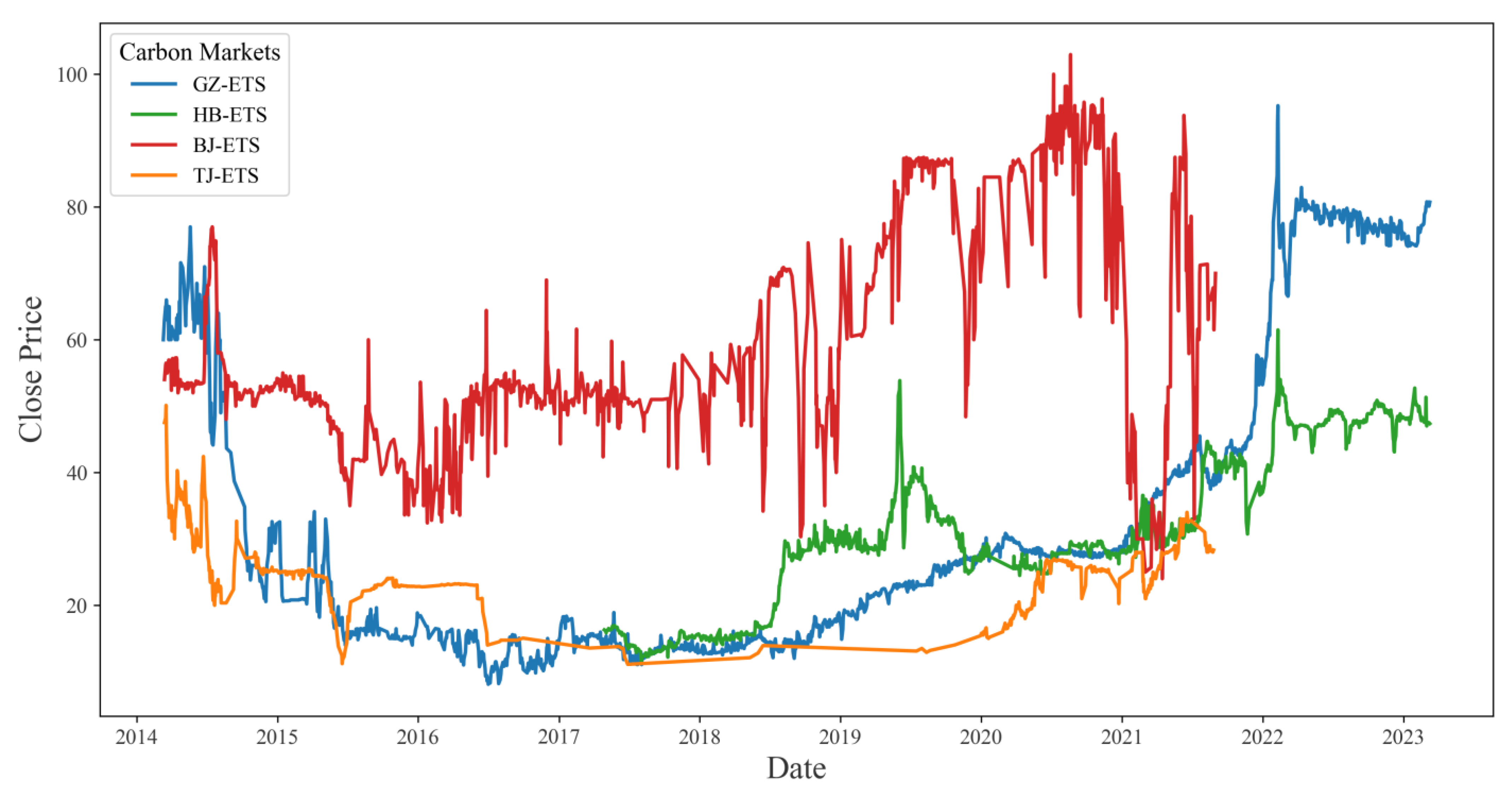
Third, the optimized SWEWT-GRU model represents a successful leakage-free time-series forecasting approach, offering reliable and accurate carbon price predictions. The model not only successfully predicts the trend of carbon trading data in the Guangzhou carbon market but also shows excellent performance in other regional carbon markets, indicating strong generalization capabilities. It offers a trajectory for developing an online carbon price forecasting model, which can facilitate precise market trend analysis for carbon market regulators and participants, thereby contributing to the sustainable growth of the carbon market.

In summary, the proposed SWEWT-GRU model demonstrates high accuracy and stability in carbon price forecasting. Its structural rationality and generalization capability have been validated, highlighting its promising application potential and reference value. However, the hybrid model proposed still has limitations. First, previous studies have shown that carbon price fluctuations are influenced by various factors, such as international markets, energy prices, and weather [5,19,24]; however, this study considers only the situation of the carbon emissions trading market itself. Second, due to hardware constraints, this study adopts the GRU model, which has a relatively simple architecture, as the basic forecasting model. It would be worthwhile to compare it with emerging models such as TimesNet [49] or Transformer [50]. Finally, the EWT decomposition scale used in this study is limited to 4. In practical situations, this may result in the discarding of high-frequency signaling components, leading to the loss of some features in the original data [31]. Further research is needed to investigate how the loss of these features may affect the model’s performance.

References

1. Wang, C.; Wang, L.; Zhao, S.; Yang, C.; Albitar, K. The Impact of Fintech on Corporate Carbon Emissions: Towards Green and Sustainable Development. Bus. Strateg. Environ. 2024. [Google Scholar] [CrossRef]
2. Li, Z.; Yang, L.; Zhou, Y.; Zhao, K.; Yuan, X. Scenario Simulation of the EU Carbon Price and Its Enlightenment to China. Sci. Total Environ. 2020, 723, 137982. [Google Scholar] [CrossRef] [PubMed]
3. Qin, Q.; Huang, Z.; Zhou, Z.; Chen, Y.; Zhao, W. Hodrick–Prescott Filter-Based Hybrid ARIMA–SLFNs Model with Residual Decomposition Scheme for Carbon Price Forecasting. Appl. Soft Comput. 2022, 119, 108560. [Google Scholar] [CrossRef]
4. Lin, B.; Jia, Z. Impacts of Carbon Price Level in Carbon Emission Trading Market. Appl. Energy 2019, 239, 157–170. [Google Scholar] [CrossRef]
5. Pan, D.; Zhang, C.; Zhu, D.; Hu, S. Carbon Price Forecasting Based on News Text Mining Considering Investor Attention. Environ. Sci. Pollut. Res. 2022, 30, 28704–28717. [Google Scholar] [CrossRef]
6. Wang, H.; Tan, Z.; Zhang, A.; Pu, L.; Zhang, J.; Zhang, Z. Carbon Market Price Prediction Based on Sequence Decomposition-Reconstruction-Dimensionality Reduction and Improved Deep Learning Model. J. Clean. Prod. 2023, 425, 139063. [Google Scholar] [CrossRef]
7. Sun, W.; Zhang, C. Analysis and Forecasting of the Carbon Price Using Multi—Resolution Singular Value Decomposition and Extreme Learning Machine Optimized by Adaptive Whale Optimization Algorithm. Appl. Energy 2018, 231, 1354–1371. [Google Scholar] [CrossRef]
8. Feng, Z.-H.; Zou, L.-L.; Wei, Y.-M. Carbon Price Volatility: Evidence from EU ETS. Appl. Energy 2011, 88, 590–598. [Google Scholar] [CrossRef]
9. Guresen, E.; Kayakutlu, G.; Daim, T.U. Using Artificial Neural Network Models in Stock Market Index Prediction. Expert Syst. Appl. 2011, 38, 10389–10397. [Google Scholar] [CrossRef]
10. Yue, W.; Zhong, W.; Xiaoyi, W.; Xinyu, K. Multi-Step-Ahead and Interval Carbon Price Forecasting Using Transformer-Based Hybrid Model. Environ. Sci. Pollut. Res. 2023, 30, 95692–95719. [Google Scholar] [CrossRef]
11. García-Martos, C.; Rodríguez, J.; Sánchez, M.J. Modelling and Forecasting Fossil Fuels, CO2 and Electricity Prices and Their Volatilities. Appl. Energy 2013, 101, 363–375. [Google Scholar] [CrossRef]
12. E, J.; Ye, J.; He, L.; Jin, H. A Denoising Carbon Price Forecasting Method Based on the Integration of Kernel Independent Component Analysis and Least Squares Support Vector Regression. Neurocomputing 2021, 434, 67–79. [Google Scholar] [CrossRef]
13. Wang, J.; Sun, X.; Cheng, Q.; Cui, Q. An Innovative Random Forest-Based Nonlinear Ensemble Paradigm of Improved Feature Extraction and Deep Learning for Carbon Price Forecasting. Sci. Total Environ. 2021, 762, 143099. [Google Scholar] [CrossRef]
14. Zhu, B.; Wei, Y. Carbon Price Forecasting with a Novel Hybrid ARIMA and Least Squares Support Vector Machines Methodology. Omega 2013, 41, 517–524. [Google Scholar] [CrossRef]
15. Zhao, Y.; Zhao, H.; Li, B.; Wu, B.; Guo, S. Point and Interval Forecasting for Carbon Trading Price: A Case of 8 Carbon Trading Markets in China. Environ. Sci. Pollut. Res. Int. 2022, 30, 49075–49096. [Google Scholar] [CrossRef] [PubMed]
16. Wang, J.; Cui, Q.; Sun, X. A Novel Framework for Carbon Price Prediction Using Comprehensive Feature Screening, Bidirectional Gate Recurrent Unit and Gaussian Process Regression. J. Clean. Prod. 2021, 314, 128024. [Google Scholar] [CrossRef]
17. Li, H.; Huang, X.; Zhou, D.; Cao, A.; Su, M.; Wang, Y.; Guo, L. Forecasting Carbon Price in China: A Multimodel Comparison. Int. J. Environ. Res. Public Health 2022, 19, 6217. [Google Scholar] [CrossRef]
18. Yang, P.; Wang, Y.; Zhao, S.; Chen, Z.; Li, Y. A Carbon Price Hybrid Forecasting Model Based on Data Multi-Scale Decomposition and Machine Learning. Environ. Sci. Pollut. Res. 2022, 30, 3252–3269. [Google Scholar] [CrossRef]
19. Zhu, B.; Wan, C.; Wang, P.; Chevallier, J. Forecasting Carbon Market Volatility with Big Data. Ann. Oper. Res. 2023, 325, 1–27. [Google Scholar] [CrossRef]
20. Huang, Y.; Dai, X.; Wang, Q.; Zhou, D. A Hybrid Model for Carbon Price Forecasting Using GARCH and Long Short-Term Memory Network. Appl. Energy 2021, 285, 116485. [Google Scholar] [CrossRef]
21. Huang, Y.; He, Z. Carbon Price Forecasting with Optimization Prediction Method Based on Unstructured Combination. Sci. Total. Environ. 2020, 725, 138350. [Google Scholar] [CrossRef]
22. Liu, H.; Shen, L. Forecasting Carbon Price Using Empirical Wavelet Transform and Gated Recurrent Unit Neural Network. Carbon Manag. 2020, 11, 25–37. [Google Scholar] [CrossRef]
23. Yan, K.; Li, C.; Zhao, R.; Zhang, Y.; Duan, H.; Wang, W. Predicting the Ammonia Nitrogen of Wastewater Treatment Plant Influent via Integrated Model Based on Rolling Decomposition Method and Deep Learning Algorithm. Sustain. Cities Soc. 2023, 94, 104541. [Google Scholar] [CrossRef]
24. Qi, S.; Cheng, S.; Tan, X.; Feng, S.; Zhou, Q. Predicting China’s Carbon Price Based on a Multi-Scale Integrated Model. Appl. Energy 2022, 324, 119784. [Google Scholar] [CrossRef]
25. Zhou, F.; Huang, Z.; Zhang, C. Carbon Price Forecasting Based on CEEMDAN and LSTM. Appl. Energy 2022, 311, 118601. [Google Scholar] [CrossRef]
26. Xu, Y.; Che, J.; Xia, W.; Hu, K.; Jiang, W. A Novel Paradigm: Addressing Real-Time Decomposition Challenges in Carbon Price Prediction. Appl. Energy 2024, 364, 123126. [Google Scholar] [CrossRef]
27. Li, D.; Li, Y.; Wang, C.; Chen, M.; Wu, Q. Forecasting Carbon Prices Based on Real-Time Decomposition and Causal Temporal Convolutional Networks. Appl. Energy 2023, 331, 120452. [Google Scholar] [CrossRef]
28. Chen, Y.; Yu, S.; Islam, S.; Lim, C.P.; Muyeen, S.M. Decomposition-Based Wind Power Forecasting Models and Their Boundary Issue: An in-Depth Review and Comprehensive Discussion on Potential Solutions. Energy Rep. 2022, 8, 8805–8820. [Google Scholar] [CrossRef]
29. Quilty, J.; Adamowski, J. Addressing the Incorrect Usage of Wavelet-Based Hydrological and Water Resources Forecasting Models for Real-World Applications with Best Practices and a New Forecasting Framework. J. Hydrol. 2018, 563, 336–353. [Google Scholar] [CrossRef]
30. Fang, W.; Huang, S.; Ren, K.; Huang, Q.; Huang, G.; Cheng, G.; Li, K. Examining the Applicability of Different Sampling Techniques in the Development of Decomposition-Based Streamflow Forecasting Models. J. Hydrol. 2019, 568, 534–550. [Google Scholar] [CrossRef]
31. Gao, R.; Du, L.; Suganthan, P.N.; Zhou, Q.; Yuen, K.F. Random Vector Functional Link Neural Network Based Ensemble Deep Learning for Short-Term Load Forecasting. Expert Syst. Appl. 2022, 206, 117784. [Google Scholar] [CrossRef]
32. Zhu, J.; Yang, M.; Ren, Z.J. Machine Learning in Environmental Research: Common Pitfalls and Best Practices. Environ. Sci. Technol. 2023, 57, 17671–17689. [Google Scholar] [CrossRef] [PubMed]
33. Ding, L.; Zhang, R.; Zhao, X. Forecasting Carbon Price in China Unified Carbon Market Using a Novel Hybrid Method with Three-Stage Algorithm and Long Short-Term Memory Neural Networks. Energy 2024, 288, 129761. [Google Scholar] [CrossRef]
34. Gilles, J. Empirical Wavelet Transform. IEEE Trans. Signal Process. 2013, 61, 3999–4010. [Google Scholar] [CrossRef]
35. Liu, Q.; Cao, J.; Zhang, J.; Zhong, Y.; Ba, T.; Zhang, Y. Short-Term Power Load Forecasting in FGSM-Bi-LSTM Networks Based on Empirical Wavelet Transform. IEEE Access 2023, 11, 105057–105068. [Google Scholar] [CrossRef]
36. Cho, K.; van Merrienboer, B.; Bahdanau, D.; Bengio, Y. On the Properties of Neural Machine Translation: Encoder-Decoder Approaches. arXiv 2014, arXiv:1409.1259. [Google Scholar] [CrossRef]
37. Hochreiter, S.; Schmidhuber, J. Long Short-Term Memory. Neural Comput. 1997, 9, 1735–1780. [Google Scholar] [CrossRef]
38. Chung, J.; Gulcehre, C.; Cho, K.; Bengio, Y. Empirical Evaluation of Gated Recurrent Neural Networks on Sequence Modeling. arXiv 2014, arXiv:1412.3555. [Google Scholar] [CrossRef]
39. Lin, H.; Chen, C.; Huang, G.; Jafari, A. Stock Price Prediction Using Generative Adversarial Networks. J. Comput. Sci. 2020, 17, 188–196. [Google Scholar] [CrossRef]
40. Klaar, A.C.R.; Stefenon, S.F.; Seman, L.O.; Mariani, V.C.; Coelho, L. dos S. Optimized EWT-Seq2Seq-LSTM with Attention Mechanism to Insulators Fault Prediction. Sensors 2023, 23, 3202. [Google Scholar] [CrossRef]
41. Rong, G.; Li, K.; Su, Y.; Tong, Z.; Liu, X.; Zhang, J.; Zhang, Y.; Li, T. Comparison of Tree-Structured Parzen Estimator Optimization in Three Typical Neural Network Models for Landslide Susceptibility Assessment. Remote Sens. 2021, 13, 4694. [Google Scholar] [CrossRef]
42. Du, L.; Gao, R.; Suganthan, P.N.; Wang, D.Z.W. Bayesian Optimization Based Dynamic Ensemble for Time Series Forecasting. Inf. Sci. 2022, 591, 155–175. [Google Scholar] [CrossRef]
43. Cao, J.; Li, Z.; Li, J. Financial Time Series Forecasting Model Based on CEEMDAN and LSTM. Physica A 2019, 519, 127–139. [Google Scholar] [CrossRef]
44. Lo, A.Y.; Mai, L.Q.; Lee, A.K.; Francesch-Huidobro, M.; Pei, Q.; Cong, R.; Chen, K. Towards Network Governance? The Case of Emission Trading in Guangdong, China. Land Use Policy 2018, 75, 538–548. [Google Scholar] [CrossRef]
45. Cheung, Y.-W.; Lai, K.S. Lag Order and Critical Values of the Augmented Dickey–Fuller Test. J. Bus. Econ. Stat. 1995, 13, 277–280. [Google Scholar] [CrossRef]
46. Jarque, C.M.; Bera, A.K. Efficient Tests for Normality, Homoscedasticity and Serial Independence of Regression Residuals. Econ. Lett. 1980, 6, 255–259. [Google Scholar] [CrossRef]
47. Xu, K.; Xia, Z.; Cheng, M.; Tan, X. Carbon Price Prediction Based on Multiple Decomposition and XGBoost Algorithm. Environ. Sci. Pollut. Res. 2023, 30, 89165–89179. [Google Scholar] [CrossRef]
48. Aguiar-Conraria, L.; Soares, M.J. The Continuous Wavelet Transform: Moving beyond Uni- and Bivariate Analysis. J. Econ. Surv. 2013, 28, 344–375. [Google Scholar] [CrossRef]
49. Zuo, C.; Wang, J.; Liu, M.; Deng, S.; Wang, Q. An Ensemble Framework for Short-Term Load Forecasting Based on TimesNet and TCN. Energies 2023, 16, 5330. [Google Scholar] [CrossRef]
50. Liu, Y.; Wu, H.; Wang, J.; Long, M. Non-Stationary Transformers: Exploring the Stationarity in Time Series Forecasting. arXiv 2022, arXiv:2205.14415. [Google Scholar] [CrossRef]
Figure 1. Working steps of the SWEWT algorithm.
Energies 17 04358 g001
Figure 2. Basic network structure of GRU.
Energies 17 04358 g002
Figure 3. Workflow of the proposed SWEWT-GRU model.
Energies 17 04358 g003
Figure 4. Closing price of the GDEA.
Energies 17 04358 g004
Figure 5. ACF and PACF images of the carbon price.
Energies 17 04358 g005
Figure 6. Decomposition results of the data with varying lengths.
Energies 17 04358 g006
Figure 7. Forecasting results of the SWEWT-GRU model.
Energies 17 04358 g007
Figure 8. Forecasting results of models with different structures.
Energies 17 04358 g008
Figure 9. Forecasting results of models with different levels of data leakage.
Energies 17 04358 g009
Figure 10. Visualization of carbon prices in different carbon markets.
Energies 17 04358 g010