Structural Effects of Economic Shocks on the Macroeconomic Economy–Electricity–Emissions Nexus in India via Long-Term Cointegration Approach

Abstract

For developing nations to achieve net-zero targets, macroeconomic linkages impacting the decoupling of emissions from economic growth must account for non-linear business cycles and economic shocks. This study aims to delineate decarbonization policy pathways for the Indian electricity sector in the aftermath of COVID-19 by analysing the long-term evolution of the economy–electricity–emissions (3E) nexus during the 2008 financial crisis and during COVID-19, covering the period of 1996Q2 to 2020Q3. Upon testing multiple theoretical 3E systems, it was found that a model internalizing trade, inflation, and stochasticity was able to minimize the reproduction errors from growth to recession phases, as well as predict the rebound effect from an economic crisis. This was revealed to be due to more information within the coefficients in a trade stochastic model. Our results confirm the existence of electricity-associated emission decoupling with capital formation in the long-run, post-crisis, while economic growth and inflation increase CO₂ emissions. The main finding highlights the negative feedback loop of inflation->trade->emissions, which shows that GDP and emissions are not directly causal. This long-run macroeconomic dynamic death spiral causes decoupling to be inhibited, where fossil fuel imports should not be subsidized for economic shock rebound, and the risk hedging of energy transition investments should occur in the post-COVID-19 era.

1. Introduction

It is a challenge for modern economic policies to decouple energy production from carbon emissions in order to combat Human-Caused Climate Change (HCCC). The case for an economy in its developing phase is that energy use, specifically electricity generation, occurs primarily from fossil fuels (FFs), like coal and oil [1]. This is especially true due to the structural integration of FFs with economic growth ever since the industrial revolution, with all developed nations of the world banking on FF use to power their economies over the past century [2,3]. With HCCC having palpable and long-term detrimental effects on the environment, it is economically difficult to structurally decouple FFs and introduce alternative clean energy, such as renewable energy (RE), for electricity generation in developing economies, like India and China [1,4,5,6]. Both India and China have large populations and a fast-growing economy, which is dependent on tremendous amounts of energy generation to keep the economic machinery functioning [7]. Rapid structural change can lead to drastic short-term socioeconomic shocks, making energy transition a non-straightforward solution [3].

Decoupling is achievable not only by clean RE, which involves intermittent sources like wind and solar energy [3,8], but also by advancing cleaner generation from oil and gas and increasing production efficiency [9]. However, continual technological advancement needs innovation, which must be powered by economic growth, implying that there needs to be an incentive for the same. From a macroeconomic perspective, levels of CO₂ emissions can be an indicator of the propensity for energy transition [8]. As a result, most macroeconomic models measure decoupling as either energy intensity reduction or emission intensity reduction [3]. However, it has been argued in the literature that the Gross Domestic Product (GDP) is not necessarily an indicator for growth [10], with studies often pointing that the total capital is what determines the capability to innovate [11]. Thus, the first issue within an economy–electricity–emissions (3E) nexus is to establish the behaviour of how each macroeconomic determinant affects CO₂ emission levels with the complexity of the GDP, capital, and even international trade being part of dynamic feedback systems [12,13,14]. This paper attempts to create several control systems to approximate the real-world behaviour of the Indian 3E system to gauge the exact level of decoupling in electricity generation.

The second aspect of this paper tackles the main deficiency in the current literature. While GDP is treated by existing econometric models as linear or exponential while estimating the causality with emissions [3,14,15], higher-order phenomena are seen in economic growth. Specifically, bi-stage cyclic patterns of growth and recession in business cycles are prevalent [16]. At the peak of a business cycle, interest rates are the lowest, leading to expanding GDP growth and simultaneous energy use, which also causes inflation [17]. It may be pointed out that innovation also hits a peak at this point. However, to control inflation, interest rates are risen by federal banks, which contracts the GDP and production (ultimately energy use), termed as the recession phase [16]. To the best of our knowledge, the existing research fails to address how the decoupling of emissions in power generation changes within the business cycle. Thus, the second target of this paper is to empirically analyse various 3E control systems to identify the dynamics of CO₂ emissions in business cycle phases and their relationship to macroeconomic variables. For achieving decoupling in a developing economy, it is imperative to identify how the status of decarbonization changes in the higher-order behaviour of economic systems [6,9].

The third issue of measuring the decarbonization of electricity in developing countries is the impact of exogenous shocks on the incentive of decoupling, which has not been addressed in the macroeconomic literature. For example, the sub-prime mortgage crisis of 2008 was a global phenomenon that changed the course of RE development sharply, with Chinese solar panels overtaking Japanese and European production sharply [18]. At the same time, developing nations’ carbon emissions and the emission intensity of electricity use sharply increased post-2008 crisis [18,19], implying that there was lesser incentive to generate clean power over FF power. While many previous studies have revealed how decarbonization patterns changed in the aftermath of the 2008 crisis [18,20,21,22], the macroeconomic linkages that accelerate CO₂ emissions are not known. In the rebound of COVID-19, we have also seen a rebound of emissions. While it may be argued that COVID-19 is vastly different from the sub-prime mortgage crisis, a macroeconomic lens will visualize both crises as a sudden shock to the GDP and consumer demand [18,23,24].

This paper focuses on the causalities of the decarbonization of power generation in India in relation to macroeconomic variables and how such causalities are impacted by higher-order economic behaviour and economic shocks. India was chosen as the case study because it is the most populous country, with a significant portion of the country being below the poverty line [25], which affects the incentive for decoupling. With FF penetration increasing from 11.7 TJ (2000) to 29.6 TJ (2020) [26], more than a third of the total power generation comes from coal [27], which suggests that a fast-growing economy is not necessarily boosting RE [28]. Simultaneously, economic growth has been noticeable, with the GDP increasing by 550% in this period [29,30], notwithstanding that inflation has increased by 5.8% [31] and cumulative emissions have increased by 250% [32] from 2000 to 2020. Secondly, unlike other fast-growing developing economies like China, the 2008 crisis did not significantly contract the GDP or cumulative emissions in India [33], but CO₂ emissions decreased by 6% in the year following COVID-19 [34]. This has drastic impacts on the 3E nexus’ decarbonization efforts, which previous research has not addressed with higher-order GDP growth [3,9,20,21]. Thirdly, India is a much larger net importer of oil products than China [28], which raises the question as to how electricity-related emissions have changed in relation to Trade Openness (TROP) during higher-order movements and before and after economic shocks.

The importance of this paper is to delineate the interplay of the incentive for innovation in decoupling in the electricity sector of a fast-growing, developing economy during business cycle movements and the economic shocks of 2008 (financial crisis) and 2020 (COVID-19), such that economic policies for net-zero targets can be identified in a post-pandemic world. This research explores the key macroeconomic pathways that can eventually lead to a stable achievement of net-zero targets and the continued decarbonization of electricity generation [35]. The rest of the paper is organized as follows: Section 2 shows a literature review to introduce the theoretical basis of macroeconomic frameworks in order to build the hypothesis across economic events. Section 3 shows the methodology that is used to analyse the linkages within the 3E nexus, and Section 4 introduces the data of the analysis. Section 5 presents the results and discussions of policy implications, and Section 6 shows a robustness analysis of the results. The final section concludes the main findings of this paper.

2. Literature Review, Hypothesis Development, and Macroeconomic Frameworks

The theoretical basis for this paper lies on the inverted U-shaped Environmental Kuznets Curve (EKC) hypothesis. The ‘inverted U’ postulate of the EKC hypothesis implies that, in the initial stages of economic growth, CO₂ emissions increase, while upon economic maturity, emissions decrease [8,36]. The primary concern with this hypothesis is that there are several studies which do claim the existence of the EKC, specifically in high-income and high-RE-penetrated economies [6,8,21,24]. However, about 20% of the studies refute the existence of the EKC, mainly in developing countries [12,37,38,39]. A major gap in the literature is that most studies focus on total energy use across all sectors and do not focus specifically on electricity generation, which is responsible for the maximum energy use and emissions among the economic sectors in India [37].

The literature on the EKC can be divided into four strands. The first strand deals with reduction in the energy intensity of the economy, mainly comprising bivariate models employing energy use and GDP as the functional variables. The basis of this hypothesis lies in the fact that higher economic growth results in higher energy use, which leads to efficient methods of energy use, further increasing economic growth [40,41,42,43,44]. Granger causality has been extensively used in these studies, but mixed evidence has been found in such cases [43,44]. The second strand combines the first type with CO₂ emissions, focusing on the reduction in emission intensity. Normally, such studies are bivariate or trivariate with an energy–economy–emissions nexus approach [5,8,9,45,46], with very few studies focusing on the electricity aspect in developing countries [37,47]. One particular recent study confirmed that both economic growth and energy use significantly degraded the environment in eight developing Asian nations, including India [5]. However, the question of the extent of economic shock impact was not analysed, even though the time interval was studied extensively [5,9,45,48,49].

The third strand of the literature is a generational advancement of the EKC hypothesis. The dynamic relationships underscoring the pathways for decoupling are examined through the lens of the Cobb-Douglas production theory (which suggests that the GDP is a result of capital formation, labour, and productivity [50]). The main hypothesis of the studies is not only limited to emission intensity reduction in the GDP but is also extended to emission intensity reduction in capital formation [50]. Since productivity is ultimately a result of the efficiency of energy conversion, energy use acts as a proxy for factor productivity [45,51,52,53,54]. Labor is often proxied by employment [22,48,51,55], with one study attempting to evaluate the dynamic relationship between electricity-use and employment in India [56]. A major drawback of most studies in this strand is that the stochastic nature of labour and productivity variation with business cycles is not incorporated into these studies. More so, very few studies have tested the dynamic links with regard to electricity generation [55,56].

The final branch deals with the highly stochastic nature of trade (or TROP, as defined in most studies). TROP is non-deterministic and may have completely different trends from business cycle fluctuations, yet very few studies have addressed how the decarbonization of energy use varies with TROP during growth and recession phases. While considering a control system, multiple studies found that increased trade has a beneficial effect on the 3E nexus in the long-run, reducing emissions [57,58,59,60]. However, in terms of energy transition, increased imports can be a sign of a lack of energy security.

Within the 3E nexus, it has been stated that ‘short-term’ economic growth is aligned with ‘long-term’ decarbonization goals [18,61,62], but the macroeconomic pathway to achieve the same has not been provided. The authors of [62] argue that economic shocks change RE policy direction, but they fail to empirically show how exactly such a change is sustained in the long-run. While structural breaks do exemplify the change in policy directions [59,63], they do not explain which factor aids in the rebound of energy use and how the status of decoupling adapts. Moreover, GDP, TROP, capital, etc. needs to be pivoted to an economic shock to empirically determine the exact pathway of decarbonization in the post-crisis macroeconomy. Decarbonization has second priority compared to economic recovery after COVID-19 [23], and past studies have only shown the symptoms of COVID-19-related impact on electricity-related emissions [64,65]. A clear post-pandemic macroeconomic theory for ensuring decoupling is yet to be empirically determined.

The second gap in the literature is the focus on the specific macroeconomics of India, as the third highest global CO₂ emitter [32]. While there have been a few studies on the dynamics of electricity production and the GDP in India [4,37], no previous research has addressed how inflation affects the dynamics of electricity-related CO₂ emissions. As business cycles change inflation along with the GDP, it is imperative to also answer what the causality of CO₂ emissions and inflation is and how it changes with growth and recession phases. The existing models have mostly used a GDP deflator, ignoring how inflation specifically plays a part in decarbonization [8,9,44,47,59]. 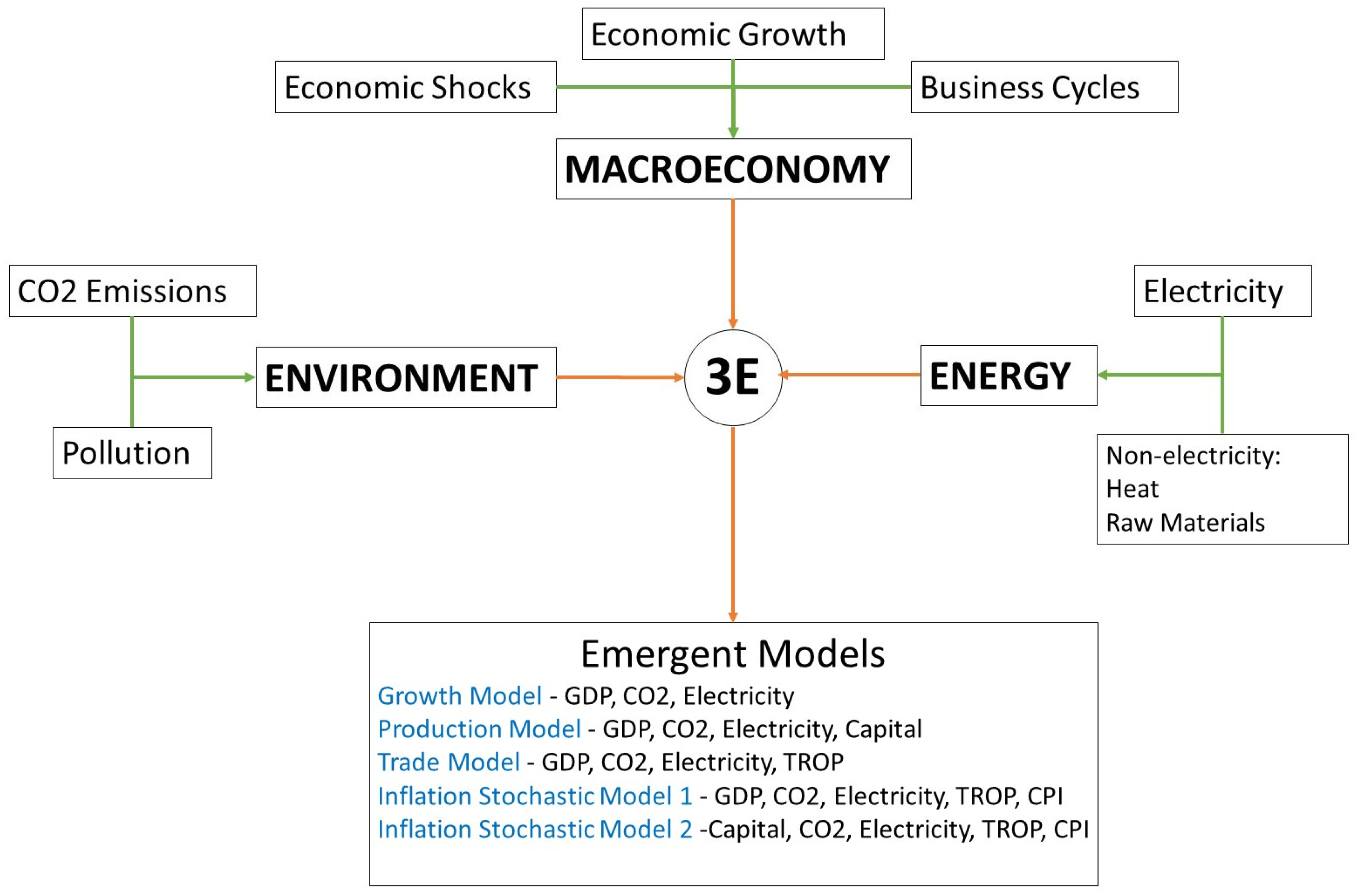Specifically, inflation increases after the rebound from a shock [61,65], but previous studies have not delineated how the feedback from inflation to the GDP to CO₂ emissions plays out. This is a key contribution of this paper, showing the dynamic links between inflation and emissions, within production and trade models, affected by the 2008 financial and COVID-19 crises in the Indian electricity sector. The modelling framework is schematically shown in Figure 1.

Within the modelling framework of Figure 1, this paper will explore five specific macroeconomic models, with specific hypotheses in regard to economic shocks. While the growth model, production theory, and trade stochasticity has been explored in the literature, this study adds inflation stochasticity to examine the specific aforementioned research gap. The 3E nexus comes with expected behaviours, and, from a macroeconomic perspective, the following hypothesis can be adopted, extending the purview of the EKC:

In business cycle movements, GDP and energy use/emissions tend to move in the same direction due to increased money supply during the growth phase, which is where interest rates tend to decrease. Similarly, this causes inflation to rise, which ultimately leads to the reversal of the cycle into the recession phase. As a result, the first hypothesis can be written as follows:

Hypothesis 1.

The decoupling of emissions from economic growth is independent of the linkage to inflation emissions.

The second consideration is one of the key foci of this study, which is economic shocks. During economic shocks, economic growth contracts, and the rebound in the economy results from production increase [18]. The incentive for decarbonization in this rebound phase (or even after a crisis) has not been explained in the past literature; therefore, we can build the second hypothesis, based on the interaction of emissions with the GDP, capital, and TROP.

Hypothesis 2.

The decoupling of emissions is inversely related between pre- and post-phases of shocks.

The third hypothesis is built around the higher-order behaviour of economic movements and the information contained in a model representing the 3E nexus. While the growth model captures the long-run behaviour of GDP-CO₂ causalities, it does not necessarily represent the impulse response as real-world behaviour [5,49,55]. We can assume that a stochastic model will represent a real-world impulse response much better than a deterministic growth model.

Hypothesis 3.

Decoupling emerges from stochasticity instead of linear relationships with the macroeconomy.

3. Materials and Methods

3.1. Modelling Specifications

The models are constructed as per Figure 1, using a long-term cointegration approach, which provides a more concrete econometric model than Vector Auto-Regression (VAR) [66,67]. As seen above, all the models are multivariate, with the dependent variable being CO₂ emissions in each case, representing the macroeconomic effects on decoupling. To account for the higher-order effects and integrating the economic shock rebound endogenously into the 3E nexus system, quarterly data are used from 1996 to 2020, encompassing both the 2008 financial crisis and the pre-crisis period for COVID-19. It must be noted that the Indian macro data are properly reported from 1996 onwards as well. All the series are first normalized to base year 2015 = 100 and then transformed into a logarithmic form to eliminate heteroskedasticity in time-series modelling [15]. Vector Error Correction Models (VECMs) incorporating long-run cointegration are quite prevalent in econometric studies [10,57], allowing for the three hypotheses to be testable. Over short samples, such as in our macroeconomic analysis, VECMs have been shown to have complex dynamic issues, such as multiple lags, difference lags, etc. [22,37,65,66,68]. This issue is dealt with by the robustness analysis method, where we use the approximate entropy method [69] to account for the amount of information present in the explanatory variables. Moreover, we compartmentalize the simulation whenever overfitting occurs in the model to make the VECM achieve a dynamic equilibrium. Both of these are novel approaches to econometric VECM modelling. The 5 models to assess the decoupling situations are given in Equations (1)–(4).

$${\mathrm{l}\mathrm{n}\Delta \mathrm{C}}_{\mathrm{t}}=\mathrm{f}({\mathrm{l}\mathrm{n}\Delta \mathrm{G}\mathrm{D}\mathrm{P}}_{\mathrm{t}},{\mathrm{l}\mathrm{n}\Delta \mathrm{E}\mathrm{l}}_{\mathrm{t}})$$

(1)

$${\mathrm{l}\mathrm{n}\Delta \mathrm{C}}_{\mathrm{t}}=\mathrm{f}({\mathrm{l}\mathrm{n}\Delta \mathrm{G}\mathrm{D}\mathrm{P}}_{\mathrm{t}},{\mathrm{l}\mathrm{n}\Delta \mathrm{K}}_{\mathrm{t}}{,\mathrm{l}\mathrm{n}\Delta \mathrm{E}\mathrm{l}}_{\mathrm{t}})$$

(2)

$${\mathrm{l}\mathrm{n}\Delta \mathrm{C}}_{\mathrm{t}}=\mathrm{f}({\mathrm{l}\mathrm{n}\Delta \mathrm{G}\mathrm{D}\mathrm{P}}_{\mathrm{t}},{\mathrm{l}\mathrm{n}\mathrm{T}\mathrm{R}\mathrm{O}\mathrm{P}}_{\mathrm{t}},{\mathrm{l}\mathrm{n}\Delta \mathrm{E}\mathrm{l}}_{\mathrm{t}})$$

(3)

$${\mathrm{l}\mathrm{n}\Delta \mathrm{C}}_{\mathrm{t}}=\mathrm{f}({\mathrm{l}\mathrm{n}\Delta \mathrm{G}\mathrm{D}\mathrm{P}}_{\mathrm{t}},{{\mathrm{l}\mathrm{n}\Delta \mathrm{T}\mathrm{R}\mathrm{O}\mathrm{P}}_{\mathrm{t}},{\mathrm{l}\mathrm{n}\Delta \mathrm{C}\mathrm{P}\mathrm{I}}_{\mathrm{t}},\mathrm{l}\mathrm{n}\Delta \mathrm{E}\mathrm{l}}_{\mathrm{t}})$$

(4a)

$${\mathrm{l}\mathrm{n}\Delta \mathrm{C}}_{\mathrm{t}}=\mathrm{f}({\mathrm{l}\mathrm{n}\Delta \mathrm{K}}_{\mathrm{t}},{{\mathrm{l}\mathrm{n}\Delta \mathrm{C}\mathrm{P}\mathrm{I}}_{\mathrm{t}},{\mathrm{l}\mathrm{n}\Delta \mathrm{T}\mathrm{R}\mathrm{O}\mathrm{P}}_{\mathrm{t}},\mathrm{l}\mathrm{n}\Delta \mathrm{E}\mathrm{l}}_{\mathrm{t}})$$

(4b)

Each of the 5 models (Figure 1) are trained over growth and recession periods from 1996Q2 to 2008Q4, and thereafter, an impulse is exogenously applied to GDP and K (where applicable) in 2009Q1, replicating the 2008 financial crisis. Such an impulse is more than the 2x standard deviation, which will allow us to test Hypothesis 3 specifically. The model is trained again from 2012Q1 to 2020Q3 to capture the pre-COVID-19 and COVID-19 impacts on the 3E nexus.

3.2. Data Specifications

The time series data from 1996Q1 to 2020Q4 that are used in this study are described in

Table 1. Modelling variables and abbreviations, data sources, and units.

Variable	Units of Measurement	Data Source
GDP	Constant 2015 US$	[70]
K (capital)	Constant 2015 US$	[70]
El (electricity generation)	Exa Joules (EJ)	[71]
TROP (trade openness)	Quarterly (%)	[70]
CPI (consumer price index)	Ratio	[70]
C (CO2 emissions)	Mega Tons (MT)	[71]

, along with the data sources.

Figure 2 graphs the data in the sampling period, and

Table 2. Descriptive statistics of the modelling variables from Figure 1.

Variable	Mean	Median	Std. Dev.	Skewness	Kurtosis
ln GDP	1.611	1.602	0.379	−0.001	−1.396
ln K	1.765	1.833	0.264	−0.268	−1.371
ln CPI	1.776	1.743	0.206	0.135	−1.400
TROP	0.395	0.409	0.109	−0.119	−1.083
ln El	1.258	1.245	0.172	0.116	−1.214
ln C	1.821	1.818	0.160	0.049	−1.430
Δln GDP	0.012	0.013	0.019	−3.873	42.97
Δln K	0.008	0.010	0.037	−1.847	39.68
Δln CPI	0.007	0.008	0.007	0.065	2.091
ΔTROP	0.001	0.002	0.023	−0.191	2.266
Δln El	0.006	0.006	0.005	0.670	6.865
Δln C	0.005	0.005	0.006	−0.246	1.468

Note: Δ represents the first differences.

gives the descriptive statistics of the data. El (electricity generation) and C (CO₂ emissions) are available as annual data and were disaggregated to quarterly data by the Denton-Cholette method [72]. TROP is calculated as the ratio of total trade (imports + exports) to GDP for each quarter. From Figure 2, it can be clearly delineated that there exist distinct higher-order phenomena in the data, even after normalizing and taking the logarithm, specifically for GDP, K (capital), CPI (inflation), and C (CO₂ emissions). It is also seen that the COVID-19 shock is much larger than the 2008 financial crisis in India. From Table 2, it is evident that inflation, emissions, and electricity-use move in a positive direction for India from the skewness and kurtosis values, implying that there is an absence of absolute decoupling in the Indian electricity sector.

3.3. Unit Root Tests

Before performing the econometric modelling and specifying the model, unit root tests need to be performed on each time series to assess the stationarity and integration order of the variables. Stationarity is absolutely required to remove the statistical uncertainty of spurious regressions [73]. The Augmented Dickey-Fuller (ADF) test has been used in a form (Equation (5)), (ii) a form with intercept (Equation (6)), and (iii) a form with intercept and trend (Equation (7)). However, the ADF test has been reported to give biased results [44]; therefore, Kwiatkowski’s KPSS test (reverse hypothesis of the ADF test) is used [74]. The non-inclusion of structural breaks in time series unit root testing by the ADF and KPSS tests has been argued to be spurious by econometricians [22,58,59]. As a result, the Zivot–Andrews structural break unit root test is used in this paper [75] to account for the changes in the time series regime. The Zivot–Andrews test is conducted in three forms in this paper: (i) one-time break in variables at the level form (Equation (8)), (ii) one-time break in the slope of the trend component (Equation (9)), and (iii) one-time break both in the intercept and trend function of the variables to be used for empirical analysis (Equation (10)) [56,75].

$${\Delta \mathrm{Y}}_{\mathrm{t}}=\mathrm{\mu }{\mathrm{Y}}_{\mathrm{t}-1}+{\displaystyle \sum _{\mathrm{i}=1}^{\mathrm{k}}}{\mathsf{\delta }}_{\mathrm{i}}{\Delta \mathrm{Y}}_{\mathrm{t}-\mathrm{i}}+{\mathsf{\epsilon }}_{\mathrm{t}}$$

(5)

$${\Delta \mathrm{Y}}_{\mathrm{t}}={\mathsf{\alpha }}_0+\mathrm{\mu }{\mathrm{Y}}_{\mathrm{t}-1}+{\displaystyle \sum _{\mathrm{i}=1}^{\mathrm{k}}}{\mathsf{\delta }}_{\mathrm{i}}{\Delta \mathrm{Y}}_{\mathrm{t}-\mathrm{i}}+{\mathsf{\epsilon }}_{\mathrm{t}}$$

(6)

$${\Delta \mathrm{Y}}_{\mathrm{t}}={\mathsf{\alpha }}_0+{\mathsf{\beta }}_0\mathrm{t}+\mathrm{\mu }{\mathrm{Y}}_{\mathrm{t}-1}+{\displaystyle \sum _{\mathrm{i}=1}^{\mathrm{k}}}{\mathsf{\delta }}_{\mathrm{i}}{\Delta \mathrm{Y}}_{\mathrm{t}-\mathrm{i}}+{\mathsf{\epsilon }}_{\mathrm{t}}$$

(7)

where Y represents a time series, t is the time period sampling interval, ${\mathsf{\alpha }}_0$ is the intercept, ${\mathsf{\beta }}_0$ is the coefficient for the time trend, µ is the coefficient of the lagged value of the time series at the level, $\mathsf{\delta }$ is the coefficient of the lagged value of the time series at first difference, k is the optimal lag length, and ${\mathsf{\epsilon }}_{\mathrm{t}}$ is the random walk error term. The null hypothesis, $\mathrm{\mu }=0$, is agreed when there is no unit root against the alternate hypothesis of $\mathrm{\mu }<0$, when there is a unit root present.

$${\Delta \mathrm{Y}}_{\mathrm{t}}={\mathrm{a}}_0+{\mathrm{b}}_0\mathrm{t}+{\mathrm{a}}_0{\mathrm{Y}}_{\mathrm{t}-1}+{\mathrm{b}}_0{\mathrm{D}\mathrm{U}}_{\mathrm{t}}+{\displaystyle \sum _{\mathrm{i}=1}^{\mathrm{k}}}{\mathsf{\delta }}_{\mathrm{i}}{\Delta \mathrm{Y}}_{\mathrm{t}-\mathrm{i}}+{\mathsf{\epsilon }}_{\mathrm{t}}$$

(8)

$${\Delta \mathrm{Y}}_{\mathrm{t}}={\mathrm{b}}_0+{\mathrm{c}}_0\mathrm{t}+{\mathrm{b}}_0{\mathrm{Y}}_{\mathrm{t}-1}+{\mathrm{c}}_0{\mathrm{D}\mathrm{T}}_{\mathrm{t}}+{\displaystyle \sum _{\mathrm{i}=1}^{\mathrm{k}}}{\mathsf{\delta }}_{\mathrm{i}}{\Delta \mathrm{Y}}_{\mathrm{t}-\mathrm{i}}+{\mathsf{\epsilon }}_{\mathrm{t}}$$

(9)

$${\Delta \mathrm{Y}}_{\mathrm{t}}={\mathrm{c}}_0+{\mathrm{c}}_0\mathrm{t}+{\mathrm{c}}_0{\mathrm{Y}}_{\mathrm{t}-1}+{\mathrm{d}}_0{\mathrm{D}\mathrm{U}}_{\mathrm{t}}+{\mathrm{d}}_0{\mathrm{D}\mathrm{T}}_{\mathrm{t}}+{\displaystyle \sum _{\mathrm{i}=1}^{\mathrm{k}}}{\mathsf{\delta }}_{\mathrm{i}}{\Delta \mathrm{Y}}_{\mathrm{t}-\mathrm{i}}+{\mathsf{\epsilon }}_{\mathrm{t}}$$

(10)

where ${\mathrm{D}\mathrm{U}}_{\mathrm{t}}$ is a dummy variable representing the existence of a mean shift with the time break, while ${\mathrm{D}\mathrm{T}}_{\mathrm{t}}$ shows that there is a trend shift with the time break. Equation (11) shows the conditions for the hypothesis confirmation of unit root presence.

$${\mathrm{D}\mathrm{U}}_{\mathrm{t}}=\left\{\begin{array}{c}1 \mathrm{i}\mathrm{f} \mathrm{t}>\mathrm{T}\mathrm{B}\\ 0 \mathrm{i}\mathrm{f} \mathrm{t}<\mathrm{T}\mathrm{B}\end{array}\right. \mathrm{a}\mathrm{n}\mathrm{d} {\mathrm{D}\mathrm{T}}_{\mathrm{t}}=\left\{\begin{array}{c}\mathrm{t}-\mathrm{T}\mathrm{B} \mathrm{i}\mathrm{f} \mathrm{t}>\mathrm{T}\mathrm{B}\\ 0 \mathrm{i}\mathrm{f} \mathrm{t}<\mathrm{T}\mathrm{B}\end{array}\right.$$

(11)

The null hypothesis of the unit root break date is ${\mathrm{c}}_0=0$, which indicates that the series is not stationary with a trend of not having information about the structural break point, while the ${\mathrm{c}}_0<0$ hypothesis implies that the variable is found to be trend-stationary, with one unknown time break. The Zivot-Andrews unit root tests all points as a potential break-point and estimates through regression for all possible break points successively. For both the ADF and Zivot-Andrews tests, the optimum lag order is selected based on the established Akaike Information Criterion (AIC) [76] and Bayesian Information Criterion (BIC) [77].

3.4. VECM Dynamic Cointegration Modelling

The ARDL bounds test for cointegration has been used extensively in past studies to identify the causalities in macroeconomic nexuses [8,15,36,44]. While a distributed lag-model has numerous advantages of information preservation, it has the potential of breakdown when an impulse of greater than 2x standard deviation is applied (analogy for an economic shock) [78]. Therefore, this study requires a model that can not only maintain the long-run dynamics of a 3E nexus but also approximate the rebound from the economic shock. An adaptive Vector Error Correction Model (a-VECM) is introduced in this paper, which performs a least error-path Monte Carlo simulation on the unrestricted VAR of the 5 models (Equations (1)–(5)), where the adaptive nature is to freely switch between the 5 Johansen cointegration methods (

Table 3. The five methods to determine cointegration in the models by Johansen test [66].

Model	Error Correction Term (ECT)	Cointegrated Series	Data
H2	AB′yt−1	No intercept, no trend	No trend
H1*	A(B′yt−1 + c0)	Intercept, no trend	No trend
H1	A(B′yt−1 + c0) + c1	Intercept, no trend	Linear trend
H*	A(B′yt−1 + c0 + d0t) + c1	Intercept, linear trend	Linear trend
H	A(B′yt−1 + c0 + d0t)+c1 + d1t	Intercept, linear trend	Quadratic trend

) [66] according to the least error of the subsequent stage. Equations (12)–(16) show the a-VECM for the 5 models of Equations (1)–(5).

$$\begin{array}{c}{\Delta \mathrm{C}}_{\mathrm{t}}={\mathsf{\alpha }}_0+{\mathrm{e}\mathrm{c}\mathrm{t}}_{\mathrm{C}}{\mathrm{C}}_{\mathrm{t}-1}+{\mathrm{e}\mathrm{c}\mathrm{t}}_{\mathrm{G}\mathrm{D}\mathrm{P}}{\mathrm{G}\mathrm{D}\mathrm{P}}_{\mathrm{t}-1}+{\mathrm{e}\mathrm{c}\mathrm{t}}_{\mathrm{E}\mathrm{l}}{\mathrm{E}\mathrm{l}}_{\mathrm{t}-1}+{\displaystyle \sum _{\mathrm{i}=1}^{\mathrm{n}}}{\mathsf{\alpha }}_{\mathrm{i}}{\Delta \mathrm{C}}_{\mathrm{t}-\mathrm{i}}\\ +{\displaystyle \sum _{\mathrm{j}=1}^{\mathrm{n}}}{\mathsf{\alpha }}_{\mathrm{j}}{\Delta \mathrm{G}\mathrm{D}\mathrm{P}}_{\mathrm{t}-\mathrm{j}}+{\displaystyle \sum _{\mathrm{k}=1}^{\mathrm{n}}}{\mathsf{\alpha }}_{\mathrm{k}}{\Delta \mathrm{E}\mathrm{l}}_{\mathrm{t}-\mathrm{k}}+{\mathsf{\epsilon }}_{\mathrm{t}}\end{array}$$

(12)

$$\begin{array}{c}{\Delta \mathrm{C}}_{\mathrm{t}}={\mathsf{\alpha }}_0+{\mathrm{e}\mathrm{c}\mathrm{t}}_{\mathrm{C}}{\mathrm{C}}_{\mathrm{t}-1}+{\mathrm{e}\mathrm{c}\mathrm{t}}_{\mathrm{G}\mathrm{D}\mathrm{P}}{\mathrm{G}\mathrm{D}\mathrm{P}}_{\mathrm{t}-1}+{\mathrm{e}\mathrm{c}\mathrm{t}}_{\mathrm{K}}{\mathrm{K}}_{\mathrm{t}-1}+{\mathrm{e}\mathrm{c}\mathrm{t}}_{\mathrm{E}\mathrm{l}}{\mathrm{E}\mathrm{l}}_{\mathrm{t}-1}+{\displaystyle \sum _{\mathrm{i}=1}^{\mathrm{n}}}{\mathsf{\alpha }}_{\mathrm{i}}{\Delta \mathrm{C}}_{\mathrm{t}-\mathrm{i}}\\ +{\displaystyle \sum _{\mathrm{j}=1}^{\mathrm{n}}}{\mathsf{\alpha }}_{\mathrm{j}}{\Delta \mathrm{G}\mathrm{D}\mathrm{P}}_{\mathrm{t}-\mathrm{j}}+{\displaystyle \sum _{\mathrm{k}=1}^{\mathrm{n}}}{\mathsf{\alpha }}_{\mathrm{k}}{\Delta \mathrm{K}}_{\mathrm{t}-\mathrm{k}}+{\displaystyle \sum _{\mathrm{l}=1}^{\mathrm{n}}}{\mathsf{\alpha }}_{\mathrm{l}}{\Delta \mathrm{E}\mathrm{l}}_{\mathrm{t}-\mathrm{l}}+{\mathsf{\epsilon }}_{\mathrm{t}}\end{array}$$

(13)

$$\begin{array}{l}{\Delta \mathrm{C}}_{\mathrm{t}}={\mathsf{\alpha }}_0+{\mathrm{e}\mathrm{c}\mathrm{t}}_{\mathrm{C}}{\mathrm{C}}_{\mathrm{t}-1}+{\mathrm{e}\mathrm{c}\mathrm{t}}_{\mathrm{G}\mathrm{D}\mathrm{P}}{\mathrm{G}\mathrm{D}\mathrm{P}}_{\mathrm{t}-1}+{\mathrm{e}\mathrm{c}\mathrm{t}}_{\mathrm{T}\mathrm{R}\mathrm{O}\mathrm{P}}{\mathrm{T}\mathrm{R}\mathrm{O}\mathrm{P}}_{\mathrm{t}-1}+{\mathrm{e}\mathrm{c}\mathrm{t}}_{\mathrm{E}\mathrm{l}}{\mathrm{E}\mathrm{l}}_{\mathrm{t}-1}\\ \hspace{1em}\hspace{1em}\hspace{1em}\hspace{1em}\hspace{1em}+{\displaystyle \sum _{\mathrm{i}=1}^{\mathrm{n}}}{\mathsf{\alpha }}_{\mathrm{i}}{\Delta \mathrm{C}}_{\mathrm{t}-\mathrm{i}}\\ \hspace{1em}\hspace{1em}\hspace{1em}\hspace{1em}\hspace{1em}+{\displaystyle \sum _{\mathrm{j}=1}^{\mathrm{n}}}{\mathsf{\alpha }}_{\mathrm{j}}{\Delta \mathrm{G}\mathrm{D}\mathrm{P}}_{\mathrm{t}-\mathrm{j}}+{\displaystyle \sum _{\mathrm{k}=1}^{\mathrm{n}}}{\mathsf{\alpha }}_{\mathrm{k}}{\Delta \mathrm{T}\mathrm{R}\mathrm{O}\mathrm{P}}_{\mathrm{t}-\mathrm{k}}+{\displaystyle \sum _{\mathrm{l}=1}^{\mathrm{n}}}{\mathsf{\alpha }}_{\mathrm{l}}{\Delta \mathrm{E}\mathrm{l}}_{\mathrm{t}-\mathrm{l}}+{\mathsf{\epsilon }}_{\mathrm{t}}\end{array}$$

(14)

$$\begin{array}{l}{\Delta \mathrm{C}}_{\mathrm{t}}={\mathsf{\alpha }}_0+{\mathrm{e}\mathrm{c}\mathrm{t}}_{\mathrm{C}}{\mathrm{C}}_{\mathrm{t}-1}+{\mathrm{e}\mathrm{c}\mathrm{t}}_{\mathrm{G}\mathrm{D}\mathrm{P}}{\mathrm{G}\mathrm{D}\mathrm{P}}_{\mathrm{t}-1}+{\mathrm{e}\mathrm{c}\mathrm{t}}_{\mathrm{T}\mathrm{R}\mathrm{O}\mathrm{P}}{\mathrm{T}\mathrm{R}\mathrm{O}\mathrm{P}}_{\mathrm{t}-1}+{\mathrm{e}\mathrm{c}\mathrm{t}}_{\mathrm{C}\mathrm{P}\mathrm{I}}{\mathrm{C}\mathrm{P}\mathrm{I}}_{\mathrm{t}-1}\\ \hspace{1em}\hspace{1em}\hspace{1em}\hspace{1em}\hspace{1em}+{\mathrm{e}\mathrm{c}\mathrm{t}}_{\mathrm{E}\mathrm{l}}{\mathrm{E}\mathrm{l}}_{\mathrm{t}-1}+{\displaystyle \sum _{\mathrm{i}=1}^{\mathrm{n}}}{\mathsf{\alpha }}_{\mathrm{i}}{\Delta \mathrm{C}}_{\mathrm{t}-\mathrm{i}}+{\displaystyle \sum _{\mathrm{j}=1}^{\mathrm{n}}}{\mathsf{\alpha }}_{\mathrm{j}}{\Delta \mathrm{G}\mathrm{D}\mathrm{P}}_{\mathrm{t}-\mathrm{j}}+{\displaystyle \sum _{\mathrm{k}=1}^{\mathrm{n}}}{\mathsf{\alpha }}_{\mathrm{k}}{\Delta \mathrm{T}\mathrm{R}\mathrm{O}\mathrm{P}}_{\mathrm{t}-\mathrm{k}}\\ \hspace{1em}\hspace{1em}\hspace{1em}\hspace{1em}\hspace{1em}+{\displaystyle \sum _{\mathrm{l}=1}^{\mathrm{n}}}{\mathsf{\alpha }}_{\mathrm{l}}{\Delta \mathrm{C}\mathrm{P}\mathrm{I}}_{\mathrm{t}-\mathrm{l}}+{\displaystyle \sum _{\mathrm{m}=1}^{\mathrm{n}}}{\mathsf{\alpha }}_{\mathrm{m}}{\Delta \mathrm{E}\mathrm{l}}_{\mathrm{t}-\mathrm{m}}+{\mathsf{\epsilon }}_{\mathrm{t}}\end{array}$$

(15)

$$\begin{array}{l}{\Delta \mathrm{C}}_{\mathrm{t}}={\mathsf{\alpha }}_0+{\mathrm{e}\mathrm{c}\mathrm{t}}_{\mathrm{C}}{\mathrm{C}}_{\mathrm{t}-1}+{\mathrm{e}\mathrm{c}\mathrm{t}}_{\mathrm{K}}{\mathrm{K}}_{\mathrm{t}-1}+{\mathrm{e}\mathrm{c}\mathrm{t}}_{\mathrm{T}\mathrm{R}\mathrm{O}\mathrm{P}}{\mathrm{T}\mathrm{R}\mathrm{O}\mathrm{P}}_{\mathrm{t}-1}+{\mathrm{e}\mathrm{c}\mathrm{t}}_{\mathrm{C}\mathrm{P}\mathrm{I}}{\mathrm{C}\mathrm{P}\mathrm{I}}_{\mathrm{t}-1}\\ \hspace{1em}\hspace{1em}\hspace{1em}\hspace{1em}\hspace{1em}+{\mathrm{e}\mathrm{c}\mathrm{t}}_{\mathrm{E}\mathrm{l}}{\mathrm{E}\mathrm{l}}_{\mathrm{t}-1}+{\displaystyle \sum _{\mathrm{i}=1}^{\mathrm{n}}}{\mathsf{\alpha }}_{\mathrm{i}}{\Delta \mathrm{C}}_{\mathrm{t}-\mathrm{i}}+{\displaystyle \sum _{\mathrm{j}=1}^{\mathrm{n}}}{\mathsf{\alpha }}_{\mathrm{j}}{\Delta \mathrm{K}}_{\mathrm{t}-\mathrm{j}}+{\displaystyle \sum _{\mathrm{k}=1}^{\mathrm{n}}}{\mathsf{\alpha }}_{\mathrm{k}}{\Delta \mathrm{T}\mathrm{R}\mathrm{O}\mathrm{P}}_{\mathrm{t}-\mathrm{k}}\\ \hspace{1em}\hspace{1em}\hspace{1em}\hspace{1em}\hspace{1em}+{\displaystyle \sum _{\mathrm{l}=1}^{\mathrm{n}}}{\mathsf{\alpha }}_{\mathrm{l}}{\Delta \mathrm{C}\mathrm{P}\mathrm{I}}_{\mathrm{t}-\mathrm{l}}+{\displaystyle \sum _{\mathrm{m}=1}^{\mathrm{n}}}{\mathsf{\alpha }}_{\mathrm{m}}{\Delta \mathrm{E}\mathrm{l}}_{\mathrm{t}-\mathrm{m}}+{\mathsf{\epsilon }}_{\mathrm{t}}\end{array}$$

(16)

where $\Delta$ is the first difference operator with the optimal lags for the differenced terms being determined by the AIC and BIC. The coefficients of the differenced terms form the short-run analysis, while the ect (error correction term) forms the long-run analysis. This selection of the ect is made dynamic by the a-VECM method, which enables the approximation of higher-order behaviour and the return to equilibrium after an exogenous shock. This study employs several diagnostic tests on the residuals of the models, starting with the test for normality by the Jarque-Bera (JB) goodness-of-fit test [79]. In the JB test, if the statistic is far from zero, the null hypothesis of normal distribution must be rejected. The Gaussian autoregressive conditional heteroscedasticity (G-ARCH) test is used to test whether the residuals have constant variance (null hypothesis accepts constant variance) [80]. The Ljung-Box Q (LBQ) test is used to test whether the autocorrelations of the sample of residuals is different from zero [81]. The null hypothesis of the LBQ test refers to the finding that the data are independently distributed.

3.5. Robustness Analysis and Approximate Entropy

The final part of the methodology is associated with checking the robustness of estimations using Equations (12)–(16) (the 5 models) pre- and post-crisis. Since sufficient macroeconomic data are available for the 2008 financial crisis, the robustness analysis cannot be applied to the COVID-19 crisis. Mean percentage errors of reproduction and forecasting are evaluated for the 5 models, along with the R-factors during the economic phases from 1996 to 2012 (as defined in Equation (17)).

$$\mathrm{R}={\displaystyle \frac{\sum |\left|{\mathrm{Y}}_{\mathrm{r}\mathrm{e}\mathrm{a}\mathrm{l}}\right|-\left|{\mathrm{Y}}_{\mathrm{e}\mathrm{s}\mathrm{t}}\right||}{\sum \left|{\mathrm{Y}}_{\mathrm{r}\mathrm{e}\mathrm{a}\mathrm{l}}\right|}}$$

(17)

where Y_real and Y_est are the real recorded and model estimate values for the dependent factors from Equations (12)–(16).

Apart from the above, the information contained in the estimated models must be measured to understand which model can most resemble the real world. For this, the principle of maximum entropy is applied to the estimated data of each model [82]. Entropy is a measure of disorder in a system (chaos), and the more chaotic or unpredictable the measurements of a system is, the more information it contains [83]. Thus, chaos in a system (time series) proves to reveal more information about the energy–economy–emissions nexus, which can be seen as the closest application of Occam’s Razor (the simplest explanation is the best one, but the explanation needs to be complete) [84]. While the principle of maximum entropy is usually applied to statistical thermodynamics, mechanics, physiology [83], etc., this is the first time (to the best of our knowledge) socio-economic VECM analysis is subject to it. The measure of chaos of the estimated time series data by the models is provided by calculating the approximate entropy of each of the estimates. Each of the estimated time series data in each model is equally spaced in time as follows:

$$\mathrm{U}\left(1\right),\mathrm{U}\left(2\right),\dots ,\mathrm{U}\left(\mathrm{N}\right)$$

(18)

where N is the raw data values. We define m as a length of run-time data (0 ≤ m ≤ N) and r as a real, positive number specifying a filtering level tolerance for accepting matches. The following sequence of vectors is then formed:

$$\mathrm{Y}\left(1\right),\mathrm{Y}\left(2\right),\dots ,\mathrm{Y}(\mathrm{N}-\mathrm{m}-1)$$

(19)

which in an m-dimensional real space defined by (after obtaining the results from Equations (12)–(16))

$$\mathrm{Y}\left(\mathrm{i}\right)=[{\Delta \mathrm{C}}_{\mathrm{t}}\left(\mathrm{i}\right),{\Delta \mathrm{C}}_{\mathrm{t}}\left(\mathrm{i}+1\right),\dots ,{\Delta \mathrm{C}}_{\mathrm{t}}\left(\mathrm{i}+\mathrm{m}-1\right)]$$

(20)

the above vector sequence is used for each magnitude of i as

$${\mathrm{C}}_{\mathrm{i}}^{\mathrm{m}}\left(\mathrm{r}\right)={\displaystyle \frac{(\mathrm{r}-\mathrm{d}\left|\mathrm{Y}\left(\mathrm{i}\right),\mathrm{Y}\left(\mathrm{j}\right)\right|)}{\mathrm{N}-\mathrm{m}+1}}$$

(21)

The functional magnitude of the m-dimensional space is defined as

$${\mathsf{\psi }}^{\mathrm{m}}(\mathrm{r})={\displaystyle \frac{1}{\mathrm{N}-\mathrm{m}+1}}{\displaystyle \sum _{\mathrm{i}=1}^{\mathrm{N}-\mathrm{m}+1}}\mathrm{l}\mathrm{o}\mathrm{g}\left({\mathrm{C}}_{\mathrm{i}}^{\mathrm{m}}\left(\mathrm{r}\right)\right)$$

(22)

In the final step, Equation (23) represents the final expression for Approximate Entropy (ApEn) calculation.

$$\mathrm{A}\mathrm{p}\mathrm{E}\mathrm{n}(\mathrm{m},\mathrm{r},\mathrm{N})={\mathsf{\psi }}^{\mathrm{m}}\left(\mathrm{r}\right)-{\mathsf{\psi }}^{\mathrm{m}+1}\left(\mathrm{r}\right)$$

(23)

where m ≥ 1, and ApEn(0, r, N)(u) = −C¹(r).

The specific econometric methods play critical roles in uncovering the higher-order dynamics of decoupling in a macroeconomic 3E nexus. The Zivot-Andrews test not only exemplifies regime shifts and structural reorientation but demarcates point of an exogenous shock in the time series of stationary data. The a-VECM seamlessly controls the long-run cointegration of key macroeconomic dynamics that are not reoriented in a regime shift but adapts to a different form of cointegration, while maintaining the directionality of feedbacks. This is an advantage over ARDL, which reorients all cointegrations in an economic shock. Multiple cointegrated relationships tend to be independent of each other, whether one reorients or not across a shock. A control system that can capture the maximum number of these independent relationships will contain more information, which is where the ApEn is a practical indicator for the same. Thus, from a methodological perspective, this paper proposes the above specific framework for analysing macroeconomic decarbonization that incorporates business cycle movements and the rebound effects of a shock.

4. Results

4.1. Unit Root Tests Results

Table 4. The results of the unit root tests (ADF and KPSS tests).

Variable	At Level		At First Difference
	ADF	KPSS	ADF	KPSS
ln GDP	−3.326 (2) c	1.284	−82.12 (0) a,*	0.279
ln K	−3.093 (2) c	1.454	−90.95 (0) a,*	0.187
ln CPI	−3.041 (1) c	1.562	−78.69 (0) a,*	0.171
TROP	−3.742 (1) c	1.681	−96.20 (0) b,*	0.214
ln El	−13.31 (1) c	1.629	−115.7 (0) a,*	0.053
ln C	−7.081 (0) c	1.183	−185.4 (1) b,*	0.099

Note: (): optimum lags for the ADF test; *: significant at 1% level; ^a: intercept and trend are 0; ^b: only trend is zero; ^c: intercept and trend are non-zero.

shows the results of the unit root tests of the ADF and KPSS tests, while

Table 5. The results of the unit root tests (Zivot-Andrews structural break test).

Variable	At Level		At First Difference
	t-Statistic	Breaks	t-Statistic	Breaks
ln GDP	−2.456 (2) c	2004Q2	−12.12 (0) *	2009Q1
ln K	−4.012 (2) c	2005Q1	−13.82 (0) *	2009Q1
ln CPI	−2.785 (1) c	2008Q3	−12.58 (0) *	2009Q2
TROP	−3.247 (1) c	2020Q2	−11.74 (0) *	2010Q2
ln El	−4.831 (1) c	2009Q2	−17.65 (0) *	2009Q3
ln C	−4.858 (0) c	2004Q4	−16.25 (1) *	2009Q1

Note: (): optimum lags for the ADF test; *: significant at 1% level; ^c: not significant.

shows the results of the Zivot-Andrews structural break unit root test. Using the unit root tests, we determine whether the variables are stationary at their first difference and what the order of integration of the explanatory and dependent variables is.

With the KPSS statistic being under 1.0, implying stationarity, it is seen that all the variables of the five models are stationary at their first differences. While there is a non-uniformity of trends and intercepts for the variables, the ADF test confirms that all the modelling variables are integrated at I(1). To mitigate the bias of ADF unit roots in small samples without structural breaks, the Zivot-Andrews test is utilized.

From Table 5, it is very interesting to observe that the structural breaks at level are scattered across the time interval, with no presence of stationarity. However, the variables show a marked break around the 2008 financial crisis at the first difference, when stationarity is detected (except for TROP, which is quite stochastic in nature). With the integration order confirmed at I(1), the a-VECM approach can be applied due to uniformity among the explanatory and dependent variables. Moreover, the presence of the structural break confirms that there would be a regime shift in all the models, which is where the least errors approximating model can be thought to represent the 3E nexus of India with higher-order phenomena.

4.2. Model Lag Order Determination and Cointegrations

Table 6. Lag length selection for the models of Equations (12)–(16) based on the AIC and BIC.

Lags	C = f(GDP,El)			C = f(GDP,K,El)			C = f(GDP,TROP,El)			C = f(GDP,TROP,CPI,El)			C = f(K,TROP,CPI,El)
	LL	AIC	BIC	LL	AIC	BIC	LL	AIC	BIC	LL	AIC	BIC	LL	AIC	BIC
0	355.56	−705.12	−699.32	484.92	−967.83	−954.10	475.47	−942.95	−935.22	638.70	−1267.4	−1257.7	600.56	−1191.1	−1181.5
1	577.96	−1131.9	−1109.0	750.43	−1460.9	−1422.6	714.18	−1388.4	−1350.1	923.86	−1787.7	−1730.4	875.48	−1691.0	−1633.6
2	588.32 *	−1134.7 *	−1109.9 *	750.92	−1433.9	−1365.7	714.93	1357.9	−1289.8	982.57	−1855.1	−1751.1	926.33	−1742.7 *	−1638.6 *
3	583.09	−1116.2	−1080.0	751.37	−1456.7	−1338.4	721.05	−1338.1	−1240.8	999.76 *	−1839.5 *	−1789.8 *	940.26 *	−1720.5	−1570.8
4	579.52	−1081.0	−1008.9	752.25 *	−1498.5 *	−1401.7 *	718.76	−1301.5	−1175.7	995.67	−1793.7	−1599.5	938.15	−1666.3	−1472.0
5	578.42	−1060.8	−973.06	747.76	−1327.5	−1173.9	720.59	−1273.2	−1119.6
6							834.60 *	−1373.2 *	−1416.1 *

*: Denotes selection of the lag order.

shows the optimal lag for each of the models using the AIC and BIC of the Unrestricted Vector Auto-Regression (UVAR) model. It has been argued in the literature that the AIC and BIC are quite reliable for small samples, compared to other lag-length selection criteria [85]. It can be seen that the simple model and the inflation stochastic models have the minimum number of lags, while the maximum lags are seen in the trade stochastic model, at six. This is quite counter-intuitive, as compared to the results of [4,12,44] for other developing economies, showing that the economic shocks have a major impact on international trade, rather than domestic economic growth.

Cointegration determination by Johansen’s test is the subsequent step in determining the interlinkages among macroeconomic variables towards electricity-related CO₂ emissions across two economic shocks in India. The two statistics used for verifying the existence of long-run cointegrations are trace and maximum eigen statistics. In the simple and production models (Equations (12) and (13)), two cointegrating relationships are found at the 5% significance level. The trade model (Equation (14)) shows a surprising result with four cointegrating relationships (at the 5% level), with the R ≤ 1 and R ≤ 2 hypotheses showing no evidence of cointegration. The inflation stochastic model (Equation (15)) has the maximum number of cointegrations at five (5% significance level), with significance for the lesser cointegrations at a 1% significance level.

Table 7. The Johansen long-run cointegration test for the five models of Figure 1 from 1996Q2 to 2008Q3.

Rank	C = f(GDP,El)		C = f(GDP,K,El)		C = f(GDP,TROP,El)		C = f(GDP,TROP,CPI,El)		C = f(K,TROP,CPI,El)
	Trace	Max Eigen	Trace	Max Eigen	Trace	Max Eigen	Trace	Max Eigen	Trace	Max Eigen
R = 0	65.45 *	40.72 *	52.92 *	28.29 **	69.79 *	43.71 *	101.2 *	40.80 *	124.5 *	54.75 *
R ≤ 1	24.73 **	17.48 **	30.63 **	21.55 **	26.08	15.67	60.41 *	22.77	69.75 *	36.32 *
R ≤ 2	7.255	7.255	13.07	12.95 ***	10.41	6.169	37.64 *	17.12 ***	33.44 **	20.76 ***
R ≤ 3			0.121	0.121	4.242 **	4.242 **	20.52 *	14.75 **	12.68	10.49
R ≤ 4							5.778 **	5.778 **	2.190	2.190

*: Significant at the 1% level. **: Significant at the 5% level. ***: Significant at the 10% level.

shows the complete Johansen cointegration results before the 2008 financial crisis, while

Table 8. The Johansen long-run cointegration test for the five models of Figure 1 from 2012Q2 to 2020Q3.

Rank	C = f(GDP,El)		C = f(GDP,K,El)		C = f(GDP,TROP,El)		C = f(GDP,TROP,CPI,El)		C = f(K,TROP,CPI,El)
	Trace	Max Eigen	Trace	Max Eigen	Trace	Max Eigen	Trace	Max Eigen	Trace	Max Eigen
R = 0	24.84	16.45	108.7 *	54.26 *	95.09 *	42.18 *	903.7 *	751.1 *	149.9 *	58.69 *
R ≤ 1	8.386	5.042	54.50 *	34.95 *	52.91 *	31.89 *	152.5 *	76.76 *	91.20 *	45.17 *
R ≤ 2	3.344 **	3.344 **	19.55 **	19.27 *	21.07 *	14.88 **	75.77 *	35.46 *	46.00 *	32.66 *
R ≤ 3			0.275	0.275	6.139 **	6.139 **	40.37 *	23.14 *	13.37	11.56
R ≤ 4							17.18 *	17.18 *	1.813	1.813

*: Significant at the 1% level. **: Significant at the 5% level.

shows it post-financial crisis recovery (from 2012Q2 to 2020Q3).

A higher rank is found to be significant for the simple growth and production models in the post-crisis period despite a lower sample size. For the stochastic models, the cointegrations are more significant in the post-crisis period, implying that the macroeconomic indicators were more closely linked in recent years than before 2008. We can partly confirm Hypothesis 2 of this research from this result, as long-run relationships imply that decoupling patterns changed with respect to capital, inflation and trade movements significantly across the economic shock. Therefore, we can provide a fresh perspective on the results of [3,4], wherein the macroeconomics of electricity generation is more FF-intensive in India, with RE generation merely being stochastic noise in macroeconomic movements since the introduction of the Paris Agreement in 2015.

4.3. a-VECM Dynamic Cointegration Results

Table 9. The a-VECM long- and short-run analysis for the five models from 1996Q2 to 2008Q3.

Variables	C = f(GDP,El)	C = f(GDP,K,El)	C = f(GDP,TROP,El)	C = f(GDP,TROP,CPI,El)	C = f(K,TROP,CPI,El)
Long-run Results:
Constant	0.141 *	−0.043 *	0.334 *	0.131	0.043 **
lnGDPt−1	0.065 *	0.051 *	0.215 *	0.067
lnKt−1		−0.077 *			0.012 ***
lnCPIt−1				−0.136	−0.075
TROPt−1			−0.062 **	0.001	0.022
lnElt−1	0.040 *	0.224 *	0.352 *	0.374 *	0.472 *
lnCt−1	−0.171 *	−0.171 *	−0.703 *	−0.372 *	−0.441 *
Short-run Results:
ΔlnGDPt−1	−0.201 *	0.525 *	−0.377 **	0.075
ΔlnKt−1		0.037			0.054
ΔlnCPIt−1				−0.632 *	−0.324 *
ΔTROPt−1			0.104 *	0.103 **	0.089 *
ΔlnElt−1	−0.029	0.283 *	0.300 **	−0.189	−0.281 *
ΔlnCt−1	0.182 ***	−0.221 **	0.404 *	0.939 *	0.602 *
Diagnostic Tests:
LL	565.96	734.94	722.15	996.87	909.61
AIC	−1099.9	−1349.9	−1228.3	−1803.7	−1719.2
BIC	−1069.7	−1238.9	−1033.2	−1626.0	−1624.6
χ2 Normal (JB)	1.342 #	0.173 #	0.662 #	0.208 #	0.788 #
χ2 Corr (LBQ)	60.49 b,***	15.99 a,#	28.92 a,***	18.98 a,#	31.40 a,***
χ2 ARCH	2.645 #	6.761 **	1.037 #	1.085 #	0.920 #

*: Significant at the 1% level. **: Significant at the 5% level. ***: Significant at the 10% level. ^#: Significant above the 10% level. ^a: 20 lags involved in the Monte Carlo Auto-correlation test. ^b: 35 lags involved in the Monte Carlo Auto-correlation test.

shows the long- and short-run results for the dependencies of emissions on macroeconomic variables from 1996Q2 to 2008Q3, while

Table 10. The a-VECM long- and short-run analysis for the five models from 2012Q2 to 2020Q3.

Variables	C = f(GDP,El)	C = f(GDP,K,El)	C = f(GDP,TROP,El)	C = f(GDP,TROP,CPI,El)	C = f(K,TROP,CPI,El)
Long-run Results:
Constant	0.427 *	−0.006	−0.034 *	NA	−0.009 *
lnGDPt−1	0.225 *	0.335 *	0.097 *	NA
lnKt−1		−0.266 *			−0.065 *
lnCPIt−1				NA	0.137 *
TROPt−1			0.312 *	NA	0.162 *
lnElt−1	−0.220 *	−0.274 *	0.497 *	NA	0.093 *
lnCt−1	−0.216 *	0.190 *	−0.652 *	NA	−0.193 *
Short-Run Results:
ΔlnGDPt−1	1.206 **	2.594 *	1.642 *	NA
ΔlnKt−1		−0.421 *			0.136 ***
ΔlnCPIt−1				NA	−0.874 *
ΔTROPt−1			−0.325 *	NA	0.006
ΔlnElt−1	0.458 *	0.441 *	−0.023	NA	0.057
ΔlnCt−1	0.260	0.177	0.472 *	NA	0.642 *
Diagnostic tests:
LL	325.91	455.19	426.73	NA	541.31
AIC	−609.82	−806.39	−749.45	NA	−972.61
BIC	−583.40	−743.01	−686.07	NA	−903.42
χ2 Normal (JB)	0.103 #	1.588 #	0.662 #	NA	2.201 #
χ2 Corr (LBQ)	15.13 a,#	16.81 a,#	28.92 a,***	NA	12.89 a,#
χ2 ARCH	0.409 #	0.004 #	1.037 #	NA	0.348 #

*: Significant at the 1% level. **: Significant at the 5% level. ***: Significant at the 10% level. ^#: Significant above the 10% level. ^a: 20 lags involved in the Monte Carlo Auto-correlation test.

shows the same for the 2012Q1 to 2020Q3 period. The adaptive nature of the a-VECM enables the change in the cointegration model type from pre-2008 crisis to post-2008 crisis, which gives a distinct advantage over ARDL, wherein the robustness of the modelling control systems can be checked across growth and recession phases and the rebound from the 2008 financial crisis in forecasting.

The a-VECM results show a significant regime shift pre- and post-2008 financial crisis in the macroeconomics of decoupling in the Indian electricity sector. It is found from Table 10 that trade stochastic inflation Model 4 is unstable in the post-financial crisis period, thereby enabling us to disregard the model as a measurement method of electricity-related decoupling in India. The long-run results (derived from the adaptive long-run cointegration) shows the marginal impacts of macroeconomic indicators in different 3E nexus systems, which bear weight for policy implication post-COVID-19 crisis for decarbonizing the power generation sector in India. In the simple growth and production models, GDP-CO₂ coupling is seen in the long-run, which intensifies from the pre-crisis to the post-crisis phase. However, decoupling is actually detected in terms of capital (K) formation, where the EKC can be confirmed as the long-run coefficient of K in Model 2 increases from −0.077 to −0.266. This means that for a 1% increase in capital, electricity-related emissions are reduced by 0.26%, which can be regarded as a ‘relative decoupling’ phase [3,58]. All these results are significant at the 1% level. However, a reverse long-run impact of TROP is seen in Model 3, where relative decoupling with C pre-2008 turns to coupling at 0.312 (significant at the 1% level) post-2011. Herein, we can confirm Hypothesis 2 of this study, where TROP couples with emissions after the financial crisis, whereas in the trade model, it was slightly decoupled (−0.062). This highlights significant issues in Indian power generation macroeconomics, where the rebound from a crisis is achieved by FF imports, hampering decoupling efforts. This is in opposition to previously established results for Asian economies, which proclaimed that TROP advancement leads to accelerated decoupling [63,86].

Hypothesis 2 with regard to TROP direction change towards C in the different economic regimes can further be consolidated by the long-run relationship between electricity generation and emissions. When considering economic and capital growth (models 1 and 2), we see a change in El->C from a positive to a negative association. This implies that capital and assets towards RE can macroeconomically reduce the emission intensity of electricity use (confirming the results of [5,49,51]). However, the long-run El->C shows high coupling (0.497 at 1% significance) in the post-2011 regime, when TROP is considered in the 3E nexus (Model 3 of Table 10), confirming that Indian electricity has increased dependency on imported FF after a crisis and in recent times. In trade stochastic Model 5, it might be thought that El->C coupling reduction from 0.472 to 0.093 (1% significant level) may indicate a stochastic reduction in electricity-related emissions, but the post-2011 regime shows that the CPI is positively coupled with C at 0.137 (1% significance level), whereas the CPI->C relation was insignificant in the pre-2008 crisis regime. Thus, it can be concluded that long-run inflation is cointegrated with CO₂ emissions, showing the existence of a macroeconomic death spiral from FF imports to inflation to emissions. This is one example of a higher-order macroeconomic phenomenon that is detected by the novel Model 5, not enumerated in any previous decoupling study for India.

The short-run dynamics reveal the quarterly and immediate impacts on decoupling. In all the 3E systems, the GDP becomes strongly coupled with C in the post-crisis period compared to the pre-2008 period. For example, in the production model, a 1% change in GDP growth will result in a 2.594% increase in the subsequent quarter’s CO₂ emissions, significant at the 1% level. However, in both economic regimes, CPI->C shows short-run decoupling, with a 1% change in the CPI, reducing CO₂ emissions by 0.874% in the post-2011 period (1% significance). In both the production Model 2 and trade Model 3 short-runs, TROP and K promote decoupling, which can be seen as critical power generation policy directions. In the short-run, we can confirm Hypothesis 1 of this study, that inflation and economic growth have similar impacts on decarbonization in the Indian electricity sector, but in inflation stochastic Model 2, GDP emissions and inflation emissions are independent of each other in the short-run. This is because the monetary policy of India does not follow business cycles, as financial budgeting sees massive changes annually in India [4,14,87], which hampers decoupling efforts. On the other hand, from stochastic models 4 and 5, it can be confirmed that inflation promotes decoupling in an immediate sense (quarterly) but actually increases emissions in the long-run due to dependency on FF imports. This result agrees with the review of decoupling nexus studies by [44] for developing economies.

The diagnostic tests show that the residual terms in all the models for dependent variable C are normally distributed in both the regimes. Some evidence of serial autocorrelation is seen for models 1, 3, and 5 in the pre-financial crisis regime, and for Model 3 in the post-crisis regime, it is seen at the 10% significance level. Production Model 2 shows strong evidence of autoregressive conditional heteroskedasticity at the 5% significance level in the pre-crisis regime. Figure 3 shows the CUSUM test figures, and Figure 4 shows the CUSUM-sq tests figures for the pre-crisis period for all the models. The CUSUM plots are all within the critical bounds, while the CUSUM-sq plots for models 2, 3, and 4 exceed the critical bounds. For Model 5, the stochasticity pushes the CUSUM-sq plot of C towards the critical limit but does not exceed it. Thus, it can be concluded from the diagnostic tests that stochastic Model 5 is the least-error statistical representation of a higher-order 3E nexus for the Indian electricity sector from the period of 1996 to 2020.

5. Robustness Discussion and Policy Implications

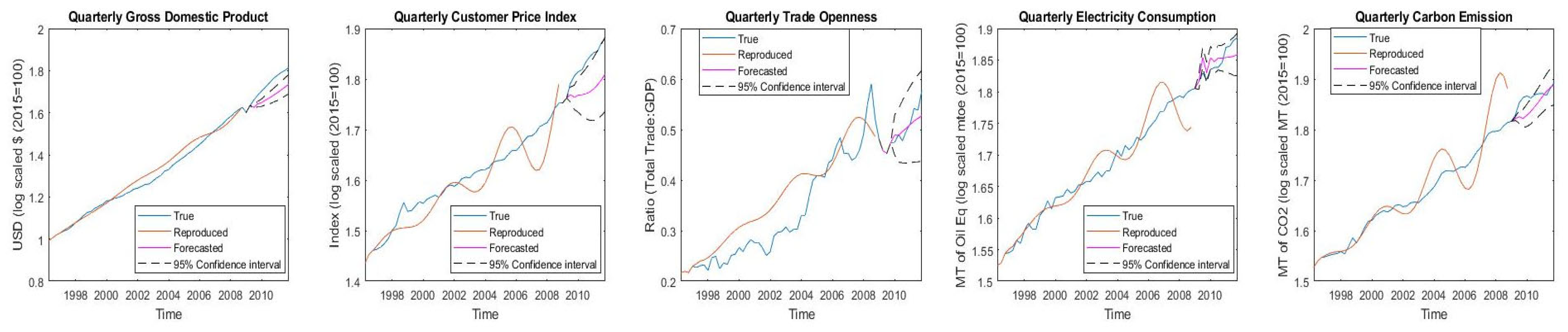
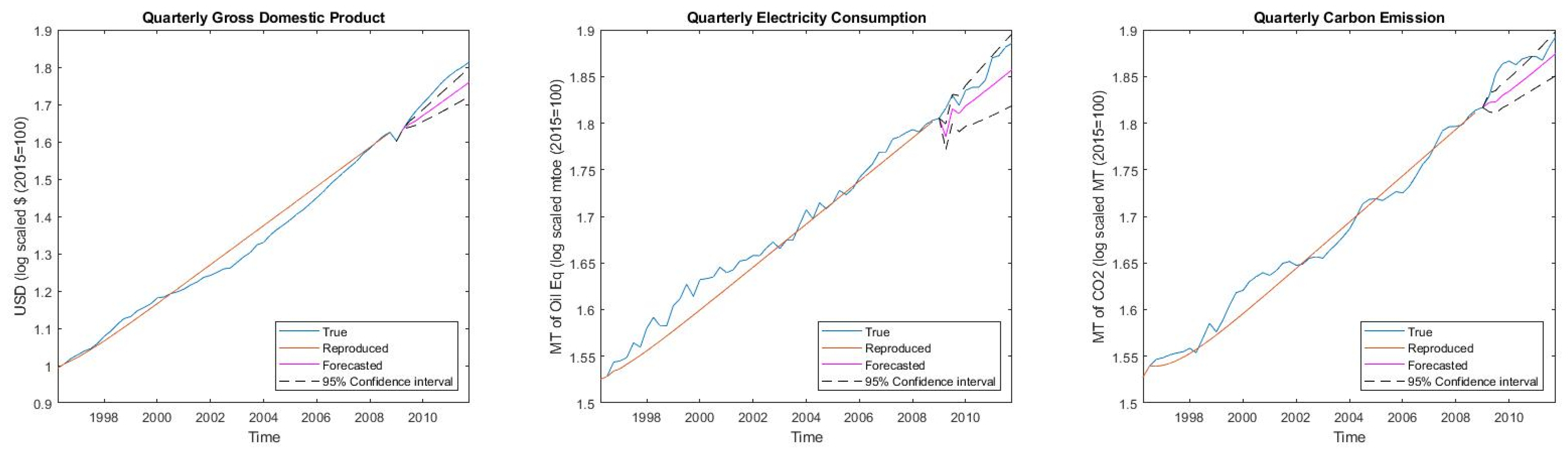
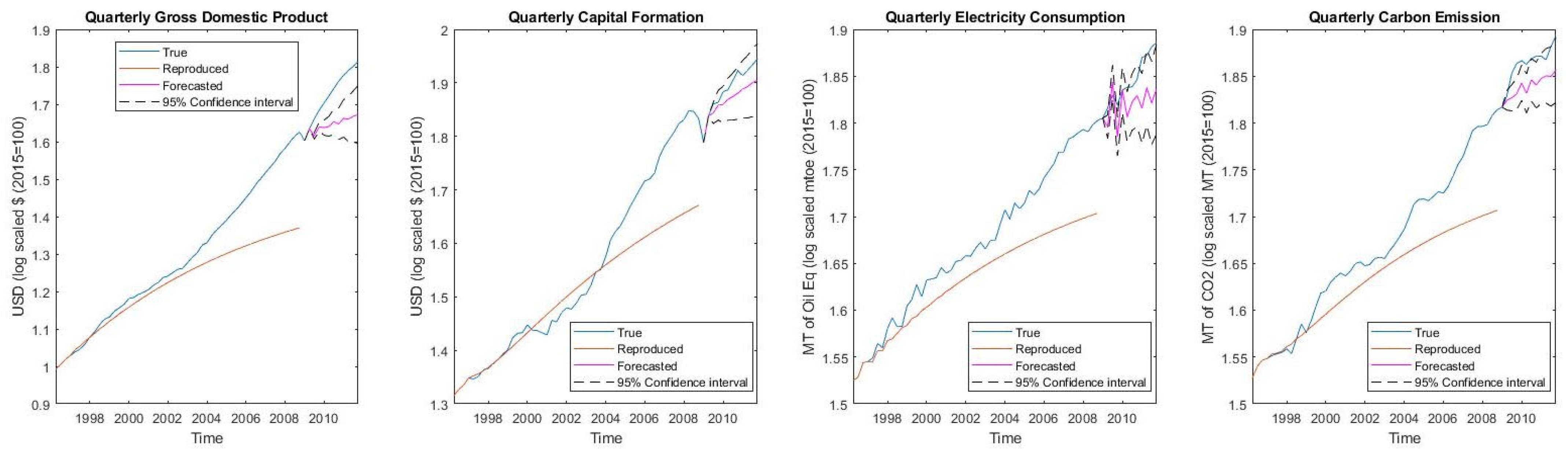
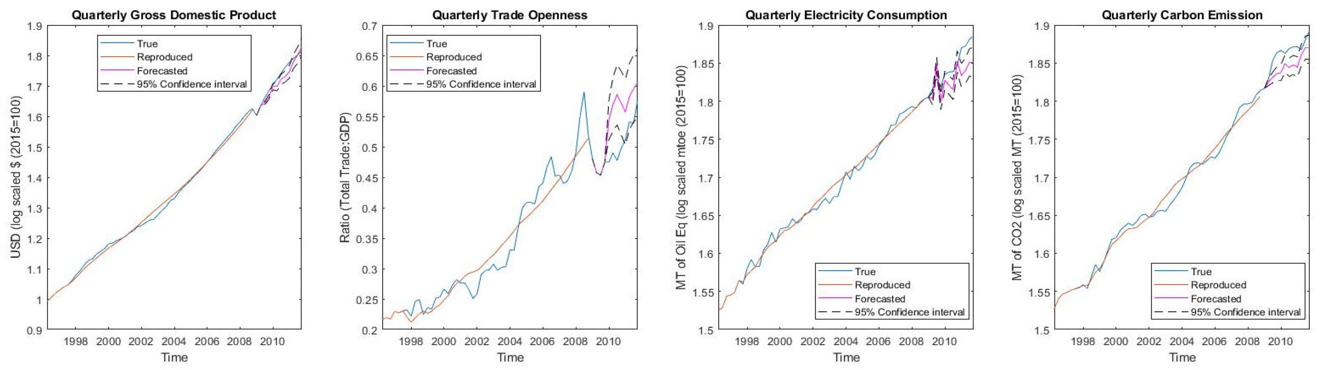
Robustness of the 3E nexus models is required to hold up against the reproduction and forecasting of business cycle movements of macroeconomic variables and rebound from the 2008 financial crisis to ascertain the results of decoupling in the electricity sector. Figure 5, Figure 6, Figure 7, Figure 8 and Figure 9 show reproduction from the 1996Q2 to 2008Q3 training period and forecasts from the 2009Q1 to 2011Q4 testing period for the five a-VECMs. Exogenous shock is applied to the GDP and K in the 2008Q4 period. The detailed coefficients of all the a-VECMs are given in Appendix A, Appendix B, Appendix C, Appendix D and Appendix E, along with the residual diagnostic tests for all the variables.

Table 11. MAPRE, MAPFE, and approximate entropy for Models 1 to 5 for training data of 1996Q2 to 2008Q4 and forecasting data from 2009Q1 to 2011Q4.

Model	MAPRE (%)	MAFRE (%)	ApEn
1 (GDP, El, C)	1.00	1.46	0.015
2 (GDP, K, El, C)	3.20	2.30	0.137
3 (GDP, TROP, El, C)	1.93	3.06	0.471
4 (GDP, CPI, TROP, El, C)	4.05	2.07	0.342
5 (K, CPI, TROP, El, C)	2.90	1.72	0.441

shows the mean aggregated percentage reproduction error (MAPRE), mean aggregated percentage forecasting error (MAPFE) and approximate entropy (ApEn) for the five models, which are the key robustness tests of this study. Specifically, ApEn is a measure of the amount of information contained in the modelled values, giving an indication of the independence of the variables in the 3E nexus considered.

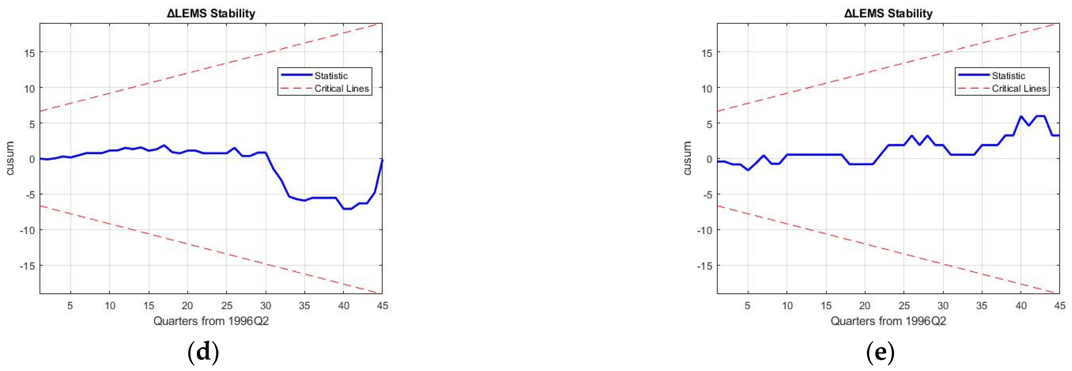
Confirming the results, Model 4 (trade stochastic 3E system) is seen to oscillate out-of-bounds in Figure 8, and Model 2 (production 3E system) is seen to reproduce large errors in Figure 6. As a result, the discussion on robustness will be limited to models 1, 3, and 5. While MAPRE of the simple growth 3E nexus is seen to be the best at an aggregated level for all the variables, ApEn is considerably less at 0.015. This implies that the amount of information in the modelling system is significantly less; it is exactly in Figure 5 where it is seen that higher-dimensional business cycle movements are not captured by this nexus. As a result, the causalities examined by previous research using the trivariate nexus of GDP-El-C can be inferred to not be representative of real-world movement [4,88,89]. Moreover, the rebound effect post-2008 crisis is also directionally opposite in the forecast for Model 1, although the forecasting error is the smallest.

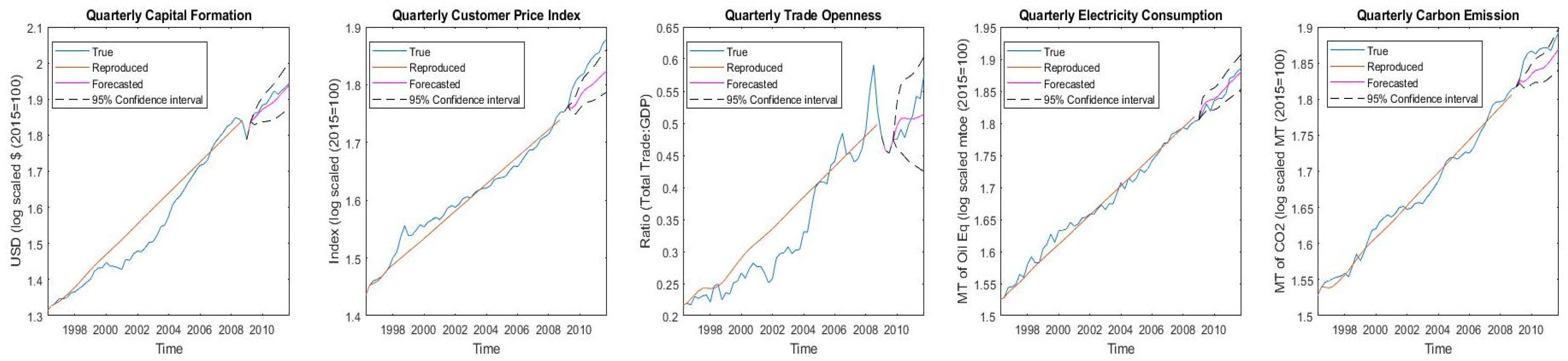
The advocacy that international trade is highly impactful on nexus modelling by the authors of [90] is highly agreeable with the results of Model 3 (Figure 7). The cyclic movements of El, C, and GDP itself is captured by the inclusion of TROP in both growth and recession periods, with a MAPRE of just 1.93%. The GDP–TROP–El–C nexus can indeed be considered an important 3E nexus policy tool with the highest entropy value of 0.47. The reason for high levels of information content in this model is that the Indian electricity sector depends on coal generation, which mainly depends on international trade. The results of [47,57,90] for the economy and electricity linkage of Italy, Ghana, and Indonesia is, thus, in agreement with the reproducibility and information quantity (entropy) of Model 3. However, the downside of the trade model is its forecasting error, which is the largest among all the considered 3E nexus systems at 3.06%, showing that the forecasting capability is limited for this model in the face of an economic shock.

Finally, inflation stochastic Model 5 has a slightly larger MAPRE than the trade Model 3 (Table 11) but still captures the cyclic movements of the variables, as seen in Figure 9. This is because the CPI (inflation) is associated with inherent stochasticity, which affects the predictive accuracy of any modelling system. Model 5 maintains a similar ApEn value as Model 3, indicating a high content of information in the modelled variables towards representing the 3E nexus for India. Where Model 5 is superior to Model 3 is in forecasting accuracy after the application of the 2008Q4 shock, which is greatly improved. Therefore, a stochastic model internalizing inflation and TROP is capable of capturing higher-dimensional business cycle movement, as well as the rebound effect of an exogenous shock better than growth, production, and trade models, confirming Hypothesis 3 of this research.

To ascertain Hypothesis 3, we utilize Equation (17) to calculate the R factors in four identified economic phases, as shown in

Table 12. Summary of the R factors (normalized) in two growth phases, one recession phase, and the recovery phase post-2008 financial crisis for models 1, 3 and 5 (models 2 and 4 contain large errors of reproducing 3E nexus data).

Economic Phase	Model	GDP	K	TROP	CPI	El	C
Growth Phase 1 (1996Q1–2000Q1)	1 (GDP, El, C)	0.010				0.011	0.006
	3 (GDP, TROP, El, C)	0.006		0.036		0.002	0.001
	5 (K, CPI, TROP, El, C)		0.009	0.021	0.036	0.012	0.016
Recession Phase 1 (2000Q2–2003Q3)	1 (GDP, El, C)	0.021				0.008	0.008
	3 (GDP, TROP, El, C)	0.009		0.066		0.004	0.005
	5 (K, CPI, TROP, El, C)		0.045	0.125	0.009	0.008	0.014
Growth Phase 2 (2003Q4–2008Q4)	1 (GDP, El, C)	0.015				0.004	0.004
	3 (GDP, TROP, El, C)	0.005		0.060		0.003	0.004
	5 (K, CPI, TROP, El, C)		0.010	0.055	0.012	0.005	0.009
Post-crisis Recovery (2008Q2–2011Q4)	1 (GDP, El, C)	0.021				0.010	0.010
	3 (GDP, TROP, El, C)	0.008		0.083		0.011	0.009
	5 (K, CPI, TROP, El, C)		0.007	0.024	0.026	0.004	0.018

An R factor greater than 0.1 shows insignificance and lesser than 0.01 shows high significance.

, with respect to models 1, 3, and 5.

R factors reveal some interesting dynamics of the capability of the models to represent higher-order business cycle movements and crisis rebound effects in different regimes. As seen in Figure 5, Figure 6, Figure 7, Figure 8 and Figure 9, the most significant R factors are reported by all the models in the first growth phase of the business cycle, at the start of the modelling period. It is in the recession phase where we see fewer significant R factors greater than 0.01 for all the modelling variables, which, again, shows improvement for models 3 and 5 in the second growth phase. Thus, it can be concluded that cointegration modelling is limited in capturing economic movement from a growth to recession phase, but it accurately predicts the opposite movement from a recession to growth phase. This is because cointegration models tend to correct errors in the direction of the overall trend in the training data, which, in this case, is an incremental direction, as opposed to the recession phase. This adds valuable insight to existing structural cointegration models [9,37,38,68]. Where Model 5 contains more significant R factors than Model 3 is in the post-crisis recovery phase, which can be attributed to the stochastic nature of the CPI and TROP being internalized to more accurately approximate the rebound from an exogenous shock to a 3E nexus system [63], affirming Hypothesis 3.

Several policy implications for the current status and future of decoupling in the Indian electricity sector can be derived from this study. Firstly, unlike previous studies in the literature where the EKC is measured solely against economic growth (GDP) [8,44,58,59], the dimensions of EKC interpretation are extended here. From 1996 to 2020, which encompasses two distinct economic periods—the pre-2008 and post-2008 financial crisis periods and multiple business cycle movements—the GDP and electricity-related CO₂ emissions are absolutely not decoupled. However, decoupling is observed through production and inflation stochastic models with respect to capital formation over a long-run cointegrated relationship. Moreover, trade openness and inflation promote decoupling in the short-run, while TROP shows evidence of coupling with emissions in the long-run. Therefore, it can be confirmed that the incentive of decoupling lies in boosting the capability of the manufacturing sector and ensuring resiliency in domestic RE markets, which builds the equity of entities invested in reducing the emission intensity of power generation [3]. Capital can also be accelerated by promoting innovation in the RE sector, which is exactly what policy programs like ‘make in India’ [91] and ‘surya ghar muft Bijli yojana’ (free electricity from rooftop solar panels) [92] aim to promote. Not only can capital formation be ensured by domestic production but also stabilized domestic markets can ensure foreign direct investment (FDI), which also boosts capital [14].

On the other hand, inflation has been rising constantly with the fast-growing GDP of India, and while short-run decoupling was seen in the post-crisis period with the CPI, it ultimately inhibited decarbonization of the electricity sector. The novel policy pathway that is uncovered in Model 5 unveils the negative feedback loop involving TROP, CPI, and emissions. Looking at

Table A23. Results of the VECM long- and short-run estimations of Model 5 pre-2008.

Independent Variable	Dependent Variable
	ΔLCAP	ΔLCPI	ΔTROP	ΔLELEC	ΔLEMS
Constant	0.001	−0.037	−0.340 *	0.082 **	0.043 **
LCAP(−1)	0.017	0.036 *	0.101 *	−0.031 *	0.012 ***
LCPI(−1)	−0.125	−0.267 *	−0.805 *	0.242 *	−0.075
TROP (−1)	−0.014	−0.045 **	−0.287 *	0.065 **	0.022
LELEC(−1)	0.350 ***	0.62 *	0.573	−0.353 **	0.472 *
LEMS(−1)	−0.238	−0.365 *	0.369	0.093	−0.441 *
ΔLCAP(−1)	0.040	0.001	0.174	0.114	0.054
ΔLCPI(−1)	−0.280	0.611 *	0.422	−0.314	−0.324 *
ΔTROP (−1)	−0.081	0.129 *	0.169	−0.119 **	0.089 *
ΔLELEC(−1)	−0.208	−0.375 *	−0.393	−0.259 ***	−0.281 *
ΔLEMS(−1)	0.345	−0.457 *	−0.604	0.193	0.602 *
Log-Likelihood	909.61
AIC	−1719.2
BIC	−1624.6
Diagnostic Tests
JB	1.103 #	0.284 #	0.200 #	0.697 #	0.788 #
Q (LBQ)	49.20 b,#	37.36 a,**	12.92 a,#	26.69 a,#	31.40 a,***
ARCH	1.658 #	2.213 #	6.661 **	0.245 #	0.920 #

*: Significant at the 1% level. **: Significant at the 5% level. ***: Significant at the 10% level. ^#: Significant above the 10% level. ^a: 20 lags involved in the Monte Carlo Auto-correlation test. ^b: 35 lags involved in the Monte Carlo Auto-correlation test.

and

Table A25. Results of the VECM long- and short-run estimations of Model 5 post-2011.

Independent Variable	Dependent Variable
	ΔLCAP	ΔLCPI	ΔTROP	ΔLELEC	ΔLEMS
Constant	0.187 *	0.098 *	−0.416 *	−0.084 *	−0.009 *
LCAP(−1)	0.122 *	−0.037 *	−0.035 *	−0.101 *	−0.065 *
LCPI(−1)	−1.242 *	−0.568 *	2.694 *	0.663 *	0.137 *
TROP (−1)	−0.100 *	0.228 *	−0.460 *	0.158 *	0.162 *
LELEC(−1)	0.705 *	0.632 *	−2.295 *	−0.258 *	0.093 *
LEMS(−1)	0.344 *	−0.124 *	−0.050 *	−0.292 *	−0.193 *
ΔLCAP(−1)	−0.610 *	0.098 ***	0.207	0.327 **	0.136 ***
ΔLCPI(−1)	−0.497 *	0.163	2.527 *	−0.892 *	−0.874 *
ΔTROP (−1)	−0.201 *	−0.139 *	0.140	−0.137 *	0.006
ΔLELEC(−1)	−0.464 *	−0.263 *	1.551 *	−0.297 **	0.057
ΔLEMS(−1)	2.105 *	−0.024	−2.421 **	0.641 **	0.642 *
ΔLCAP(−2)	−0.005	0.413 *	0.784 ***	0.682 *	0.468 *
ΔLCPI(−2)	2.990 *	−0.235 ***	−5.899 *	−0.811 **	−0.673 *
ΔTROP (−2)	−0.242 *	−0.076 *	0.426 *	−0.146 *	0.025
ΔLELEC(−2)	−0.749 *	−0.238 *	0.035	−0.406 *	−0.126
ΔLEMS(−2)	−2.180 *	−0.471 *	3.654 *	0.070	−0.195
Log-Likelihood	541.31
AIC	−972.61
BIC	−903.42
Diagnostic Tests
JB	2.144 #	5.459 **	6.302 **	0.229 #	2.201 #
Q (LBQ)	23.74 a,#	14.92 a,#	14.85 a,#	29.62 b,#	12.89 a,#
ARCH	0.803 #	0.470 #	0 #	4.700 **	0.348 #

*: Significant at the 1% level. **: Significant at the 5% level. ***: Significant at the 10% level. ^#: Significant above the 10% level. ^a: 20 lags involved in the Monte Carlo Auto-correlation test. ^b: 35 lags involved in the Monte Carlo Auto-correlation test.

, when inflation peaks and a recession phase begins, GDP growth is ensured through FF imports, which boosts TROP and ultimately reduces the CPI. However, this causes an increase in CO₂ emissions from power generation, which is where we see a long-run positive association between the CPI and TROP and between TROP and C. This resembles a death spiral with the positive effect of capital reducing CO₂ emissions during recession phases. This loop was also magnified during the rebound from the 2008 economic shock, which can also be thought to have been replicated during the COVID-19 shock, as the macroeconomic dynamics in the 3E nexus are similar to those before the 2008 financial crisis (as seen in Table 9 and Table 10). This is coupled with the fact that economic shocks destabilize RE stock markets [65], which further nullifies the positive effect of capital on decoupling, magnifying the negative feedback in the process.

6. Conclusions

This study explores the macroeconomic dynamics of decoupling in the Indian electricity sector through long-term cointegration models from 1996Q2 to 2020Q3 across the economic shocks of the 2008 financial crisis and the COVID-19 pandemic. Five models covering aspects of economic growth, Cobb-Douglas production, trade, and inflation stochasticity within the economy–electricity–emissions (3E) nexus were tested for their robustness to reproduce higher-order business cycle movements and to forecast the rebound from an economic shock. Robustness was analysed using a novel information-theory-based approximate entropy (ApEn) approach to the 3E systems and R factors in economic phases.

The key findings of the study are as follows:

• An inflation stochastic 3E system can detect higher-order behaviour in decoupling dynamics better than linear growth nexuses by containing more information in the coefficients (ApEn value of 0.441 as opposed to 0.015 of a simple growth model).
• Cointegration models can approximate decoupling and 3E dynamics more accurately in growth phases of business cycles than recession phases, with the inflation stochastic model again being superior to the other 3E systems.
• AN EKC hypothesis for the Indian electricity sector is non-existent from the period of 1996–2020 with respect to the GDP but decouples from capital growth on either side of the 2008 financial crisis.
• Inflation and TROP decoupling directions are inversely related in economic regimes across economic shocks, showing recoupling in the post-crisis regime. These factors are responsible for the rebound of the economy, at the expense of decarbonization incentives in the Indian 3E nexus.
• GDP and CO₂ emissions are not directly causal. This study found the existence of a negative feedback loop from the CPI to TROP to CO₂ emissions that inhibits the positive effect of decoupling by capital growth.

The following policy pathway can be proposed for the fast-growing, developing economy of India from the empirical evidence that was gathered in this study to ensure continued progress towards ‘net-zero’ targets in the post-COVID-19 regime:

• Risk hedging of RE investments and energy sustainability markets must be practiced during a crisis, such that the recoupling of emissions with increasing inflation in a post-crisis demand surge can be prevented.
• Macroeconomic decoupling of power generation should be tied to capital formation, rather than GDP growth incentives. Capital growth, both domestic and FDI, can accelerate RE infrastructure and introduce innovations in capacity factors, such as giga-scale solar projects and thorium-based heavy-water nuclear power reactors.
• Economic rebound should not be fostered by increased FF imports in the post-crisis period but by investments in energy transition technologies like electric vehicles and solar manufacturing, which ultimately creates capital that enables decoupling.
• Post-crisis reliance on FF imports can be reduced by removing all forms of subsidies on oil and gas sectors, such that a quick turnaround of the economy does not occur at the expense of decarbonization efforts in the electricity sector.

In terms of the limitations of this study, the tested cointegration models were not able to reproduce economic movements that lay in recession phases. Future studies should consider stochastic time series that exhibit complimentary trends during growth and recession periods, such that 3E systems are able to minimize the reproduction errors of recession phases. A second limitation is that the impact of inflation on overall energy use needs to be delineated to introduce comprehensive decoupling pathways in the face of economic shocks. More expansive theoretical bases, involving factors that were not considered in the modelling in this paper or using more critical methodological approaches, such as data assimilation, should be explored. Thirdly, the financial policies of every major developing nation are vastly different, implying that the macroeconomic dynamics of inflation and CO₂ emissions may be quite different than those of India. There are several macroeconomic dynamics that are required to be addressed in future studies for developing the progression of economies’ decoupling processes. How can social engineering be performed to artificially control inflation with a rebound effect in crisis regimes and prevent it from affecting decarbonization initiatives? The interplay of labour dynamics, wage equity, and social justice as concerns CPI-TROP-CO₂ emissions needs to be explored to determine the role of human and social capital in decoupling dynamics.

It is indeed easy to foster economic growth from imported FFs and subsidies on oil use in a post-COVID-19 recovery scenario, but this study clearly shows that such actions will inhibit decoupling in the long-run. Such short-run economic growth will ultimately lead to uneconomic growth in the pathway to achieve net-zero targets.

References

1. Ibrahim, H.A.; Ayomoh, M.K.; Bansal, R.C.; Gitau, M.N.; Yadavalli, V.S.S.; Naidoo, R. Sustainability of power generation for developing economies: A systematic review of power sources mix. Energy Strateg. Rev. 2023, 47, 101085. [Google Scholar] [CrossRef]
2. Fu, Q.; Liu, L.; Wang, H. Role of fossil fuels resources on high-quality economic development: Evidence from China. Resour. Policy 2023, 86, 104126. [Google Scholar] [CrossRef]
3. Basu, S.; Ogawa, T.; Ishihara, K.N. The methods and factors of decoupling energy usage and economic growth. In Waste-to-Energy Approaches Towards Zero Waste; Elsevier: Amsterdam, The Netherlands, 2022; pp. 269–313. [Google Scholar] [CrossRef]
4. Paul, S.; Bhattacharya, R.N. Causality between energy consumption and economic growth in India: A note on conflicting results. Energy Econ. 2004, 26, 977–983. [Google Scholar] [CrossRef]
5. Jamel, L.; Derbali, A. Do energy consumption and economic growth lead to environmental degradation? Evidence from Asian economies. Cogent Econ. Financ. 2016, 4, 1170653. [Google Scholar] [CrossRef]
6. Dong, F.; Li, J.; Wang, Y.; Zhang, X.; Zhang, S.; Zhang, S. Drivers of the decoupling indicator between the economic growth and energy-related CO2 in China: A revisit from the perspectives of decomposition and spatiotemporal heterogeneity. Sci. Total Environ. 2019, 685, 631–658. [Google Scholar] [CrossRef] [PubMed]
7. Holdren, J.P. Population and the energy problem. Popul. Environ. 1991, 12, 231–255. [Google Scholar] [CrossRef]
8. Marques, A.C.; Fuinhas, J.A.; Leal, P.A. The impact of economic growth on CO2 emissions in Australia: The environmental Kuznets curve and the decoupling index. Environ. Sci. Pollut. Res. 2018, 25, 27283–27296. [Google Scholar] [CrossRef] [PubMed]
9. Mikayilov, J.I.; Hasanov, F.J.; Galeotti, M. Decoupling of CO2 emissions and GDP: A time-varying cointegration approach. Ecol. Indic. 2018, 95, 615–628. [Google Scholar] [CrossRef]
10. Mohamed, M.M.A.; Liu, P.; Nie, G. Causality between Technological Innovation and Economic Growth: Evidence from the Economies of Developing Countries. Sustainability 2022, 14, 3586. [Google Scholar] [CrossRef]
11. Zeng, J. Reexamining the interaction between innovation and capital accumulation. J. Macroecon. 2003, 25, 541–560. [Google Scholar] [CrossRef]
12. Işik, C.; Kasımatı, E.; Ongan, S. Analyzing the causalities between economic growth, financial development, international trade, tourism expenditure and/on the CO2 emissions in Greece. Energy Sources Part B Econ. Plan. Policy 2017, 12, 665–673. [Google Scholar] [CrossRef]
13. Shahbaz, M.; Khan, S.; Tahir, M.I. The dynamic links between energy consumption, economic growth, financial development and trade in China: Fresh evidence from multivariate framework analysis. Energy Econ. 2013, 40, 8–21. [Google Scholar] [CrossRef]
14. Nepal, R.; Paija, N.; Tyagi, B.; Harvie, C. Energy security, economic growth and environmental sustainability in India: Does FDI and trade openness play a role? J. Environ. Manag. 2021, 281, 111886. [Google Scholar] [CrossRef]
15. Abbasi, K.R.; Shahbaz, M.; Jiao, Z.; Tufail, M. How energy consumption, industrial growth, urbanization, and CO2 emissions affect economic growth in Pakistan? A novel dynamic ARDL simulations approach. Energy 2021, 221, 119793. [Google Scholar] [CrossRef]
16. King, R.G.; Watson, M.W. Money, Prices, Interest Rates and the Business Cycle. Rev. Econ. Stat. 1996, 78, 35. [Google Scholar] [CrossRef]
17. Neumeyer, P.A.; Perri, F. Business cycles in emerging economies: The role of interest rates. J. Monet. Econ. 2005, 52, 345–380. [Google Scholar] [CrossRef]
18. Zhang, P.; Zhao, X.; Sun, L.; Zuo, J.; Wei, W.; Liu, X.; Peng, X.; Shan, Y.; Li, S.; Ge, L.; et al. What can we learn from the 2008 financial crisis for global power decarbonization after COVID-19? Fundam. Res. 2023, in press. [Google Scholar] [CrossRef]
19. Heffron, R.J.; Sheehan, J. Rethinking international taxation and energy policy post COVID-19 and the financial crisis for developing countries. J. Energy Nat. Resour. Law 2020, 38, 465–473. [Google Scholar] [CrossRef]
20. Piłatowska, M.; Włodarczyk, A. Decoupling Economic Growth From Carbon Dioxide Emissions in the EU Countries. Montenegrin J. Econ. 2018, 14, 7–26. [Google Scholar] [CrossRef]
21. Pao, H.-T.; Chen, C.-C. Decoupling strategies: CO2 emissions, energy resources, and economic growth in the Group of Twenty. J. Clean. Prod. 2019, 206, 907–919. [Google Scholar] [CrossRef]
22. Shahbaz, M.; Lean, H.H.; Farooq, A. Natural gas consumption and economic growth in Pakistan. Renew. Sustain. Energy Rev. 2013, 18, 87–94. [Google Scholar] [CrossRef]
23. Andrijevic, M.; Schleussner, C.-F.; Gidden, M.J.; McCollum, D.L.; Rogelj, J. COVID-19 recovery funds dwarf clean energy investment needs. Science 2020, 370, 298–300. [Google Scholar] [CrossRef] [PubMed]
24. Andreoni, V. The energy metabolism of countries: Energy efficiency and use in the period that followed the global financial crisis. Energy Policy 2020, 139, 111304. [Google Scholar] [CrossRef]
25. World Bank. Poverty Rate by Country. 2024. Available online: https://worldpopulationreview.com/country-rankings/poverty-rate-by-country (accessed on 1 May 2024).
26. IEA. World Energy Outlook, 2020. International Energy Agency. Available online: https://www.iea.org/reports/world-energy-outlook-2020 (accessed on 24 September 2023).
27. Basu, S.; Ogawa, T.; Okumura, H.; Ishihara, K.N. Assessing the geospatial nature of location-dependent costs in installation of solar photovoltaic plants. Energy Rep. 2021, 7, 4882–4894. [Google Scholar] [CrossRef]
28. International Energy Agency. India Energy Outlook. 2021. Available online: https://www.iea.org/reports/india-energy-outlook-2021 (accessed on 24 September 2023).
29. Worldometer. GDP by Country. 2023. Available online: https://www.worldometers.info/gdp/gdp-by-country/ (accessed on 24 September 2023).
30. World Bank. GDP (Current US$), India. World Development Indicators. Available online: https://data.worldbank.org/indicator/NY.GDP.MKTP.CD?locations=IN (accessed on 20 January 2024).
31. World Bank. Inflation, Consumer Prices (Annual %), India. World Development Indicators. Available online: https://data.worldbank.org/indicator/FP.CPI.TOTL.ZG?locations=IN (accessed on 20 January 2024).
32. Worldometer. CO2 Emissions by Country. 2023. Available online: https://www.worldometers.info/co2-emissions/co2-emissions-by-country/ (accessed on 24 September 2023).
33. Li, L.; Willett, T.D.; Zhang, N. The Effects of the Global Financial Crisis on China’s Financial Market and Macroeconomy. Econ. Res. Int. 2012, 2012, 961694. [Google Scholar] [CrossRef]
34. IEA. Global Energy Demand to Plunge This Year as a Result of the Biggest Shock since the Second World War; IEA: Paris, France, 2020. [Google Scholar]
35. Vogel, J.; Hickel, J. Is green growth happening? An empirical analysis of achieved versus Paris-compliant CO2–GDP decoupling in high-income countries. Lancet Planet. Health 2023, 7, e759–e769. [Google Scholar] [CrossRef] [PubMed]
36. Acaravci, A.; Ozturk, I. On the relationship between energy consumption, CO2 emissions and economic growth in Europe. Energy 2010, 35, 5412–5420. [Google Scholar] [CrossRef]
37. Ghosh, S. Electricity supply, employment and real GDP in India: Evidence from cointegration and Granger-causality tests. Energy Policy 2009, 37, 2926–2929. [Google Scholar] [CrossRef]
38. Ben Jebli, M.; Ben Youssef, S. Renewable energy consumption and agriculture: Evidence for cointegration and Granger causality for Tunisian economy. Int. J. Sustain. Dev. World Ecol. 2017, 24, 149–158. [Google Scholar] [CrossRef]
39. Lee, C.-C.; Chang, C.-P. The impact of energy consumption on economic growth: Evidence from linear and nonlinear models in Taiwan. Energy 2007, 32, 2282–2294. [Google Scholar] [CrossRef]
40. Ho, C.-Y.; Siu, K.W. A dynamic equilibrium of electricity consumption and GDP in Hong Kong: An empirical investigation. Energy Policy 2007, 35, 2507–2513. [Google Scholar] [CrossRef]
41. Yu, E.S.H.; Hwang, B.-K. The relationship between energy and GNP. Energy Econ. 1984, 6, 186–190. [Google Scholar] [CrossRef]
42. Payne, J.E. Survey of the international evidence on the causal relationship between energy consumption and growth. J. Econ. Stud. 2010, 37, 53–95. [Google Scholar] [CrossRef]
43. Payne, J.E. A survey of the electricity consumption-growth literature. Appl. Energy 2010, 87, 723–731. [Google Scholar] [CrossRef]
44. Ozturk, I. A literature survey on energy-growth nexus. Energy Policy 2010, 38, 340–349. [Google Scholar] [CrossRef]
45. Apergis, N.; Payne, J.E. CO2 emissions, energy usage, and output in Central America. Energy Policy 2009, 37, 3282–3286. [Google Scholar] [CrossRef]
46. Adedoyin, F.F.; Zakari, A. Energy consumption, economic expansion, and CO2 emission in the UK: The role of economic policy uncertainty. Sci. Total Environ. 2020, 738, 140014. [Google Scholar] [CrossRef] [PubMed]
47. Cerdeira Bento, J.P.; Moutinho, V. CO2 emissions, non-renewable and renewable electricity production, economic growth, and international trade in Italy. Renew. Sustain. Energy Rev. 2016, 55, 142–155. [Google Scholar] [CrossRef]
48. Yu, E.S.H.; Jin, J.C. Cointegration tests of energy consumption, income, and employment. Resour. Energy 1992, 14, 259–266. [Google Scholar] [CrossRef]
49. Lean, H.H.; Smyth, R. On the dynamics of aggregate output, electricity consumption and exports in Malaysia: Evidence from multivariate Granger causality tests. Appl. Energy 2010, 87, 1963–1971. [Google Scholar] [CrossRef]
50. Stern, D.I. Energy and economic growth in the USA. Energy Econ. 1993, 15, 137–150. [Google Scholar] [CrossRef]
51. Ghali, K.H.; El-Sakka, M.I.T. Energy use and output growth in Canada: A multivariate cointegration analysis. Energy Econ. 2004, 26, 225–238. [Google Scholar] [CrossRef]
52. Lee, C.-C.; Chang, C.-P.; Chen, P.-F. Energy-income causality in OECD countries revisited: The key role of capital stock. Energy Econ. 2008, 30, 2359–2373. [Google Scholar] [CrossRef]
53. Stern, D.I. A multivariate cointegration analysis of the role of energy in the US macroeconomy. Energy Econ. 2000, 22, 267–283. [Google Scholar] [CrossRef]
54. Shahbaz, M.; Zeshan, M.; Afza, T. Is energy consumption effective to spur economic growth in Pakistan? New evidence from bounds test to level relationships and Granger causality tests. Econ. Model. 2012, 29, 2310–2319. [Google Scholar] [CrossRef]
55. Narayan, P.K.; Smyth, R. Electricity consumption, employment and real income in Australia evidence from multivariate Granger causality tests. Energy Policy 2005, 33, 1109–1116. [Google Scholar] [CrossRef]
56. Raza Abbasi, K.; Hussain, K.; Abbas, J.; Fatai Adedoyin, F.; Ahmed Shaikh, P.; Yousaf, H.; Muhammad, F. Analyzing the role of industrial sector’s electricity consumption, prices, and GDP: A modified empirical evidence from Pakistan. AIMS Energy 2021, 9, 29–49. [Google Scholar] [CrossRef]
57. Abokyi, E.; Appiah-Konadu, P.; Sikayena, I.; Oteng-Abayie, E.F. Consumption of Electricity and Industrial Growth in the Case of Ghana. J. Energy 2018, 2018, 8924835. [Google Scholar] [CrossRef]
58. Tiwari, A.K.; Shahbaz, M.; Adnan Hye, Q.M. The environmental Kuznets curve and the role of coal consumption in India: Cointegration and causality analysis in an open economy. Renew. Sustain. Energy Rev. 2013, 18, 519–527. [Google Scholar] [CrossRef]
59. Shahbaz, M.; Khraief, N.; Uddin, G.S.; Ozturk, I. Environmental Kuznets curve in an open economy: A bounds testing and causality analysis for Tunisia. Renew. Sustain. Energy Rev. 2014, 34, 325–336. [Google Scholar] [CrossRef]
60. Kasman, A.; Duman, Y.S. CO2 emissions, economic growth, energy consumption, trade and urbanization in new EU member and candidate countries: A panel data analysis. Econ. Model. 2015, 44, 97–103. [Google Scholar] [CrossRef]
61. Lee, C.-C.; Wang, F.; Lou, R.; Wang, K. How does green finance drive the decarbonization of the economy? Empirical evidence from China. Renew. Energy 2023, 204, 671–684. [Google Scholar] [CrossRef]
62. Bersalli, G.; Tröndle, T.; Heckmann, L.; Lilliestam, J. Economic crises as critical junctures for policy and structural changes towards decarbonization—The cases of Spain and Germany. Clim. Policy 2024, 24, 410–427. [Google Scholar] [CrossRef]
63. Nguyen, V.M.H.; Ho, T.H.; Nguyen, L.H.; Pham, A.T.H. The Impact of Trade Openness on Economic Stability in Asian Countries. Sustainability 2023, 15, 11736. [Google Scholar] [CrossRef]
64. Adebayo, T.S.; AbdulKareem, H.K.K.; Bilal; Kirikkaleli, D.; Shah, M.I.; Abbas, S. CO2 behavior amidst the COVID-19 pandemic in the United Kingdom: The role of renewable and non-renewable energy development. Renew. Energy 2022, 189, 492–501. [Google Scholar] [CrossRef] [PubMed]
65. Basu, S.; Ishihara, K.N. Multivariate time-frequency interactions of renewable and non-renewable energy markets with macroeconomic factors in India. Energy Syst. 2023, 1–37. [Google Scholar] [CrossRef]
66. Johansen, S. Estimation and Hypothesis Testing of Cointegration Vectors in Gaussian Vector Autoregressive Models. Econometrica 1991, 59, 1551. [Google Scholar] [CrossRef]
67. Yussuf, Y.C. Cointegration test for the long-run economic relationships of East Africa community: Evidence from a meta-analysis. Asian J. Econ. Bank. 2022, 6, 314–336. [Google Scholar] [CrossRef]
68. Jordan, S.; Philips, A.Q. Cointegration Testing and Dynamic Simulations of Autoregressive Distributed Lag Models. Stata J. Promot. Commun. Stat. Stata 2018, 18, 902–923. [Google Scholar] [CrossRef]
69. Delgado-Bonal, A.; Marshak, A. Approximate Entropy and Sample Entropy: A Comprehensive Tutorial. Entropy 2019, 21, 541. [Google Scholar] [CrossRef] [PubMed]
70. Federal Bank of St. Louis (FRED). Economic Data for India. Available online: https://fred.stlouisfed.org/tags/series?t=india (accessed on 1 April 2024).
71. British Petroleum. BP Energy Outlook. 2023. Available online: https://www.bp.com/content/dam/bp/business-sites/en/global/corporate/xlsx/energy-economics/energy-outlook/bp-energy-outlook-2023-chart-data-pack.xlsx (accessed on 24 September 2023).
72. Sax, C.; Steiner, P. Temporal Disaggregation of Time Series. R J. 2013, 5, 80. [Google Scholar] [CrossRef]
73. Dickey, D.A.; Fuller, W.A. Distribution of the Estimators for Autoregressive Time Series With a Unit Root. J. Am. Stat. Assoc. 1979, 74, 427. [Google Scholar] [CrossRef]
74. Kwiatkowski, D.; Phillips, P.C.B.; Schmidt, P.; Shin, Y. Testing the null hypothesis of stationarity against the alternative of a unit root. J. Econom. 1992, 54, 159–178. [Google Scholar] [CrossRef]
75. Zivot, E.; Andrews, D.W.K. Further Evidence on the Great Crash, the Oil-Price Shock, and the Unit-Root Hypothesis. J. Bus. Econ. Stat. 2002, 20, 25–44. [Google Scholar] [CrossRef]
76. Akaike, H. Fitting autoregressive models for prediction. Ann. Inst. Stat. Math. 1969, 21, 243–247. [Google Scholar] [CrossRef]
77. Schwarz, G. Estimating the Dimension of a Model. Ann. Stat. 1978, 6, 461–464. [Google Scholar] [CrossRef]
78. Sam, C.Y.; McNown, R.; Goh, S.K. An augmented autoregressive distributed lag bounds test for cointegration. Econ. Model. 2019, 80, 130–141. [Google Scholar] [CrossRef]
79. Jarque, C.M.; Bera, A.K. A Test for Normality of Observations and Regression Residuals. Int. Stat. Rev./Rev. Int. Stat. 1987, 55, 163. [Google Scholar] [CrossRef]
80. Engle, R.F. Autoregressive Conditional Heteroscedasticity with Estimates of the Variance of United Kingdom Inflation. Econometrica 1982, 50, 987. [Google Scholar] [CrossRef]
81. Ljung, G.M.; Box, G.E.P. On a Measure of Lack of Fit in Time Series Models. Biometrika 1978, 65, 297. [Google Scholar] [CrossRef]
82. Zhao, N.; Lin, W.T. A copula entropy approach to correlation measurement at the country level. Appl. Math. Comput. 2011, 218, 628–642. [Google Scholar] [CrossRef]
83. Olbrys, J.; Majewska, E. Approximate entropy and sample entropy algorithms in financial time series analyses. Procedia Comput. Sci. 2022, 207, 255–264. [Google Scholar] [CrossRef]
84. Gill, R.D. Schrödinger’s Cat Meets Occam’s Razor. Entropy 2022, 24, 1586. [Google Scholar] [CrossRef]
85. Shan, T.A.; Rather, S.A.; Dar, H.A. Revisiting openness-growth nexus: Panel data estimates for selected developing Asian countries. Transnatl. Corp. Rev. 2024, 16, 200051. [Google Scholar] [CrossRef]
86. Nasreen, S.; Anwar, S. Causal relationship between trade openness, economic growth and energy consumption: A panel data analysis of Asian countries. Energy Policy 2014, 69, 82–91. [Google Scholar] [CrossRef]
87. International Energy Agency. Energy-Intensive economic Growth, Compounded by Unfavourable Weather, Pushed Emissions up in China and India. 2023. Available online: https://www.iea.org/reports/CO2-emissions-in-2023/ (accessed on 24 September 2023).
88. Sultan, Z.A.; Alkhateeb, T.T.Y. Energy consumption and economic growth: The evidence from India. Int. J. Energy Econ. Policy 2019, 9, 142–147. [Google Scholar] [CrossRef]
89. Ang, J.B. CO2 emissions, energy consumption, and output in France. Energy Policy 2007, 35, 4772–4778. [Google Scholar] [CrossRef]
90. Shahbaz, M.; Hye, Q.M.A.; Tiwari, A.K.; Leitão, N.C. Economic growth, energy consumption, financial development, international trade and CO2 emissions in Indonesia. Renew. Sustain. Energy Rev. 2013, 25, 109–121. [Google Scholar] [CrossRef]
91. Bhambu, M.K. Make in India and Future of Renewable Energy. SSRN Electron. J. 2015, 9, 142–147. [Google Scholar] [CrossRef]
92. KhareSaxena, A.; Saxena, S.; Sudhakar, K. Solar energy policy of India: An overview. CSEE J. Power Energy Syst. 2020. [Google Scholar] [CrossRef]
Figure 1. Modelling framework and theory schematic for analysing decoupling in the 3E (economy–electricity–emissions) nexus in India during economic shocks.
Energies 17 04354 g001
Figure 2. Graphical representation of the normalized data of (a) GDP, (b) K, (c) CPI, (d) TROP, (e) E-El, (f) C {in red—left y-axis}, and their first differences {in black—right y-axis} (modelling variables from Table 2), along with the units. The system is seen to be resilient against an economic shock (the 2008 financial crisis).
Energies 17 04354 g002
Figure 3. Plot of cumulative sum (CUSUM) of residuals for dependent variable C in the a-VECM modelling for the Indian 3E nexus from 1996Q2 to 2008Q4 for (a) Model 1 (Equation (12)), (b) Model 2 (Equation (13)), (c) Model 3 (Equation (14)), (d) Model 4 (Equation (15)), and (e) Model 5 (Equation (16)).
Energies 17 04354 g003aEnergies 17 04354 g003b
Figure 4. Plot of cumulative sum of squares (CUSUM-sq) of residuals for dependent variable C in the a-VECM modelling for the Indian 3E nexus from 1996Q2 to 2008Q4 for (a) Model 1 (Equation (12)), (b) Model 2 (Equation (13)), (c) Model 3 (Equation (14)), (d) Model 4 (Equation (15)), and (e) Model 5 (Equation (16)).
Energies 17 04354 g004
Figure 5. Reproduction of training data from 1996Q2 to 2008Q3 and forecasting of testing data from 2009Q1 to 2011Q4 by a-VECM simple growth Model 1 (GDP, El, C).
Energies 17 04354 g005
Figure 6. Reproduction of training data from 1996Q2 to 2008Q3 and forecasting of testing data from 2009Q1 to 2011Q4 by a-VECM production Model 2 (GDP, K, El, C).
Energies 17 04354 g006
Figure 7. Reproduction of training data from 1996Q2 to 2008Q3 and forecasting of testing data from 2009Q1 to 2011Q4 by a-VECM trade Model 3 (GDP, TROP, El, C).
Energies 17 04354 g007
Figure 8. Reproduction of training data from 1996Q2 to 2008Q3 and forecasting of testing data from 2009Q1 to 2011Q4 by a-VECM trade stochastic Model 4 (GDP, CPI, TROP, El, C).
Energies 17 04354 g008
Figure 9. Reproduction of training data from 1996Q2 to 2008Q3 and forecasting of testing data from 2009Q1 to 2011Q4 by a-VECM inflation stochastic Model 5 (K, CPI, TROP, El, C).
Energies 17 04354 g009