Enhanced Control Technique for Induction Motor Drives in Electric Vehicles: A Fractional-Order Sliding Mode Approach with DTC-SVM


Abstract
1. Introduction
- The stability analysis is not studied.
- Authors approximate the differential of a signal u by . They compute the fraction derivative by , which is not suitable; moreover, signal u can be negative.
2. Preliminary Steps
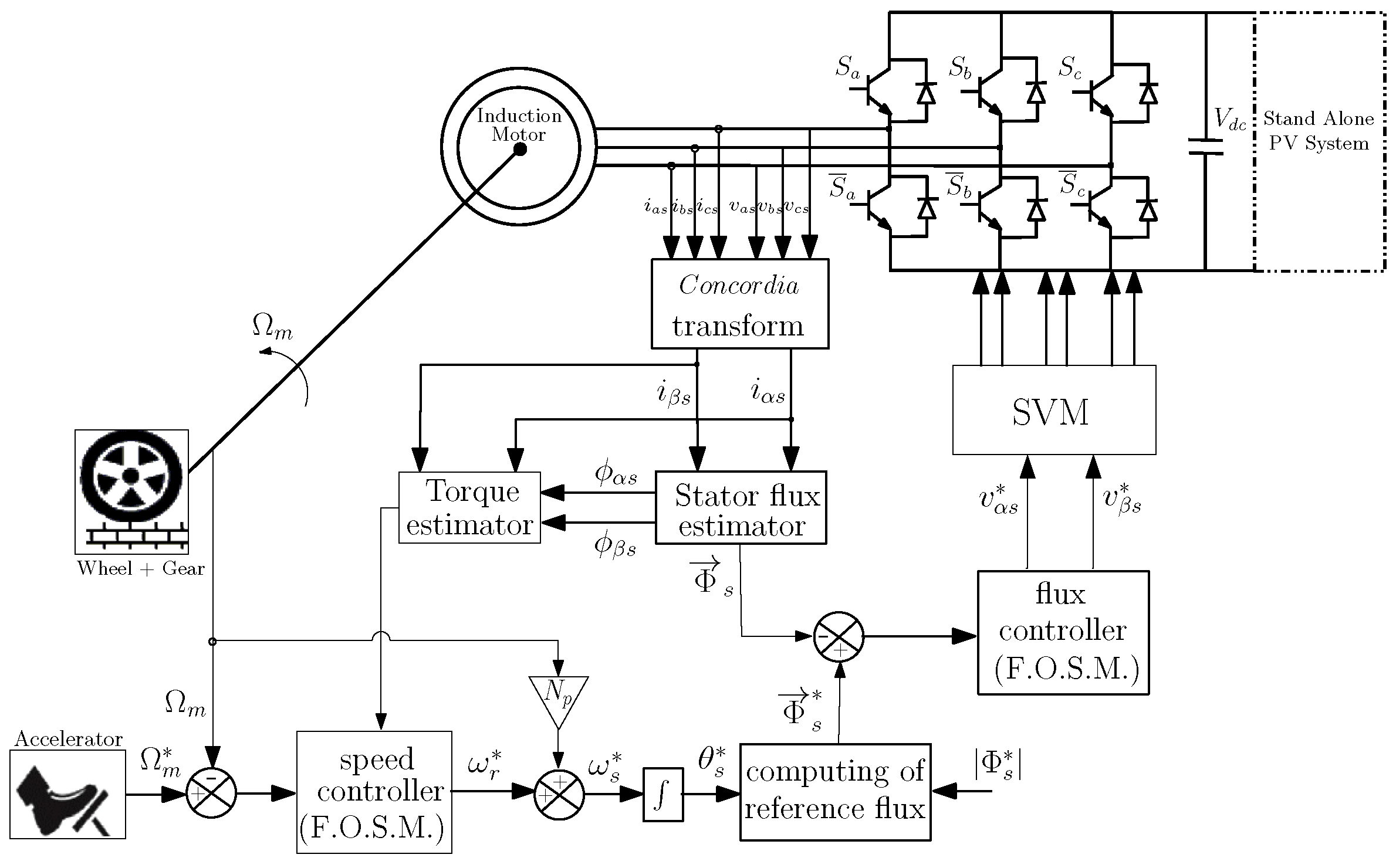
2.1. Modeling Induction Machines with DTC-SVM
2.2. Tractive Systems
- -
- Rolling resistance, the force opposing a vehicle’s motion, is calculated as . This equation shows that rolling resistance is directly proportional to the vehicle’s mass and the rolling resistance coefficient, typically around 0.005 for electric vehicle tires. Minimizing rolling resistance is crucial for maximizing energy efficiency in electric vehicles.
- -
- Aerodynamic drag, the force opposing a vehicle’s motion through the air, is calculated as . This equation shows that drag is directly proportional to air density, frontal area, drag coefficient, and the square of the vehicle’s speed. Minimizing drag is crucial for fuel efficiency, especially at higher speeds.
- -
- The force needed to climb a hill, , is calculated as , where is the slope angle. This means steeper hills and heavier vehicles require more force to climb.
2.3. Background on Fractional Calculus
3. Suggested Control Approach
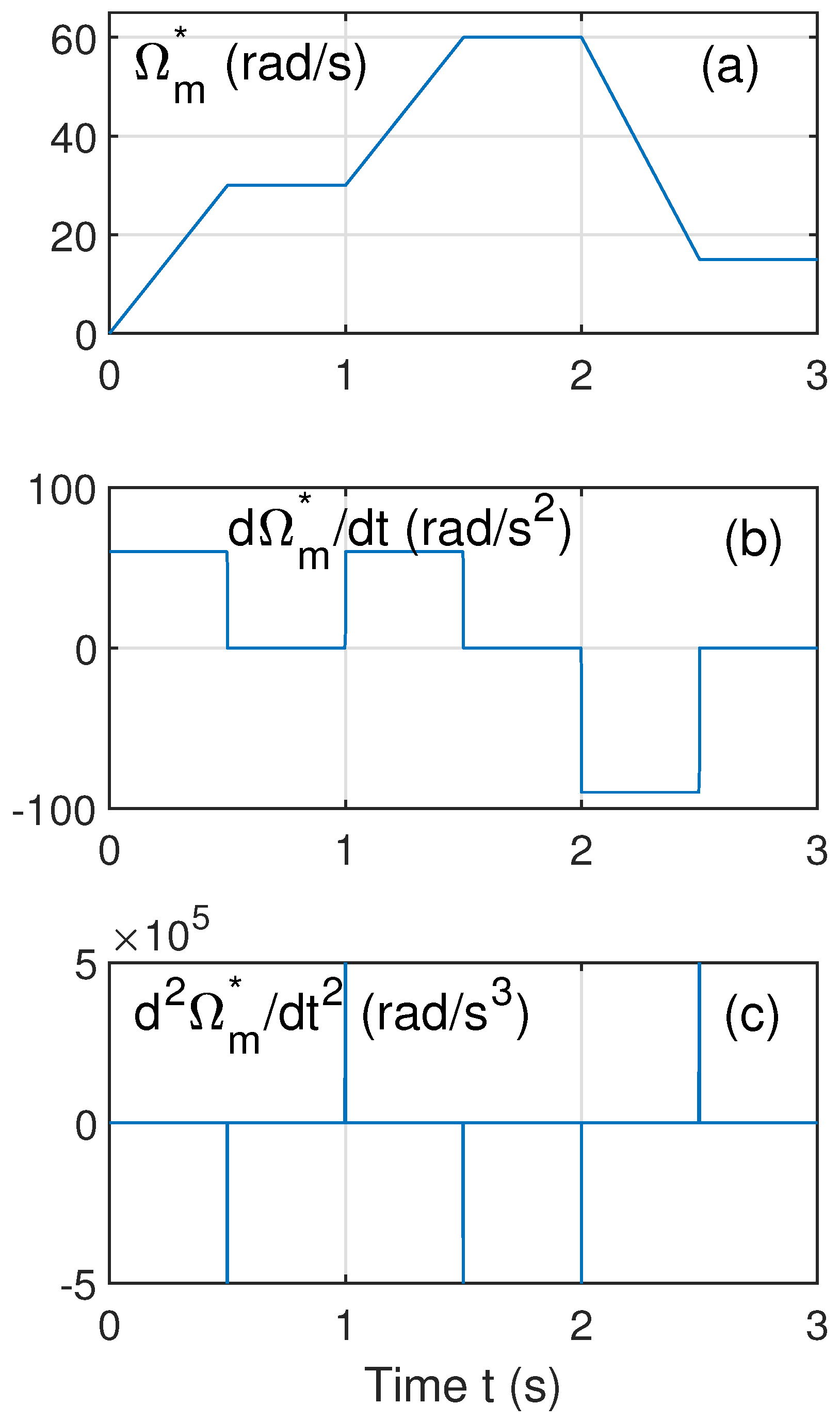
3.1. Speed Control
3.2. Flux Control
4. Evaluation of the FO-SM-DTC-SVM Method Based on Simulations Results
4.1. Evaluation Metrics
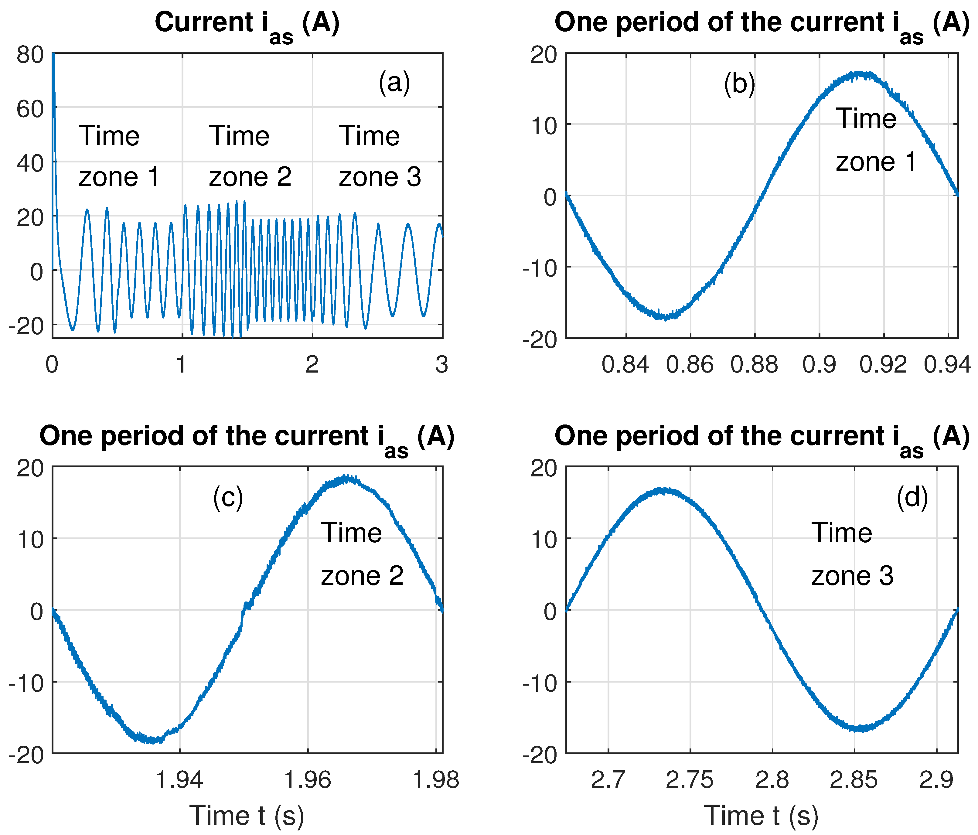
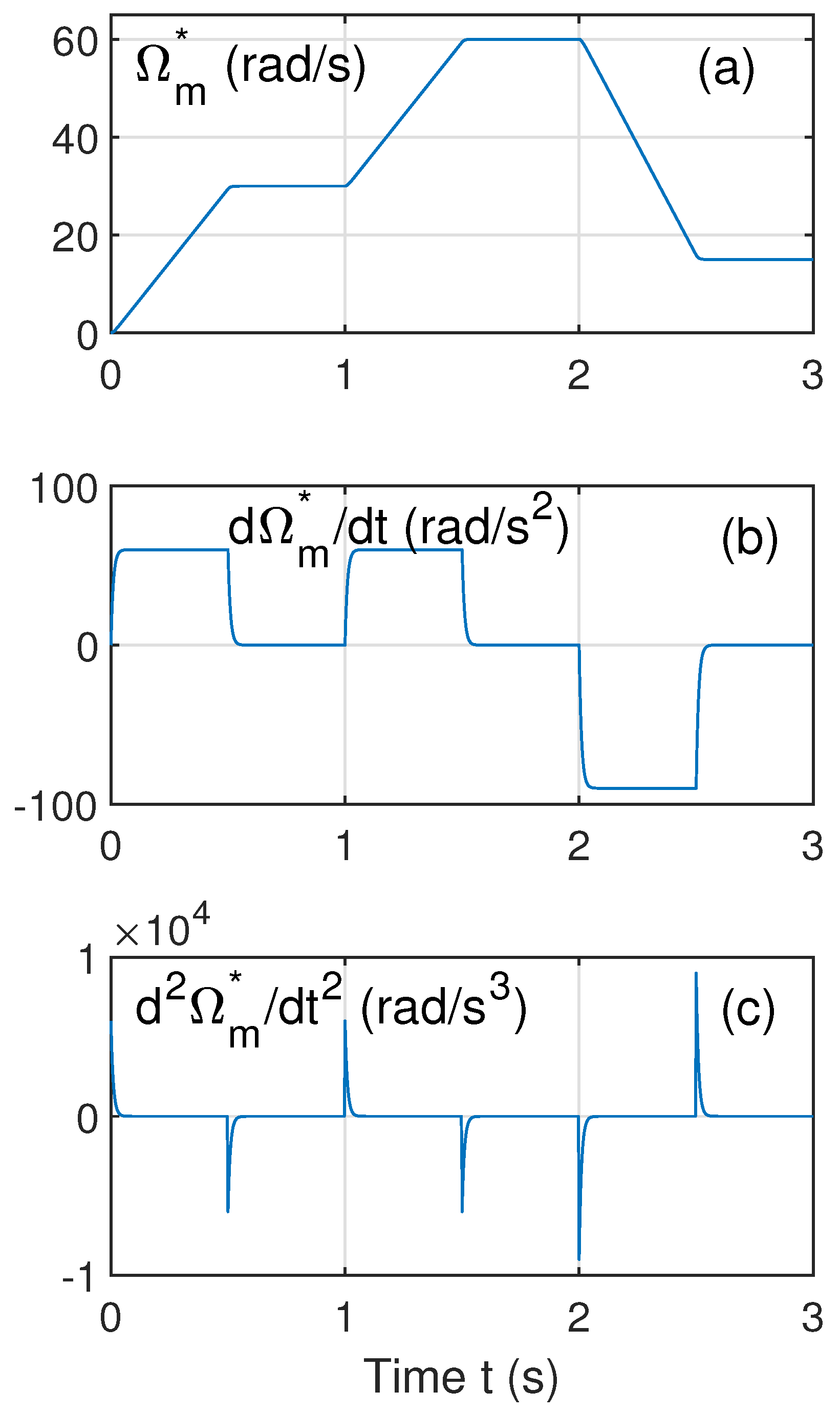
- Time zone 1: s.
- Time zone 2: s.
- Time zone 3: s.
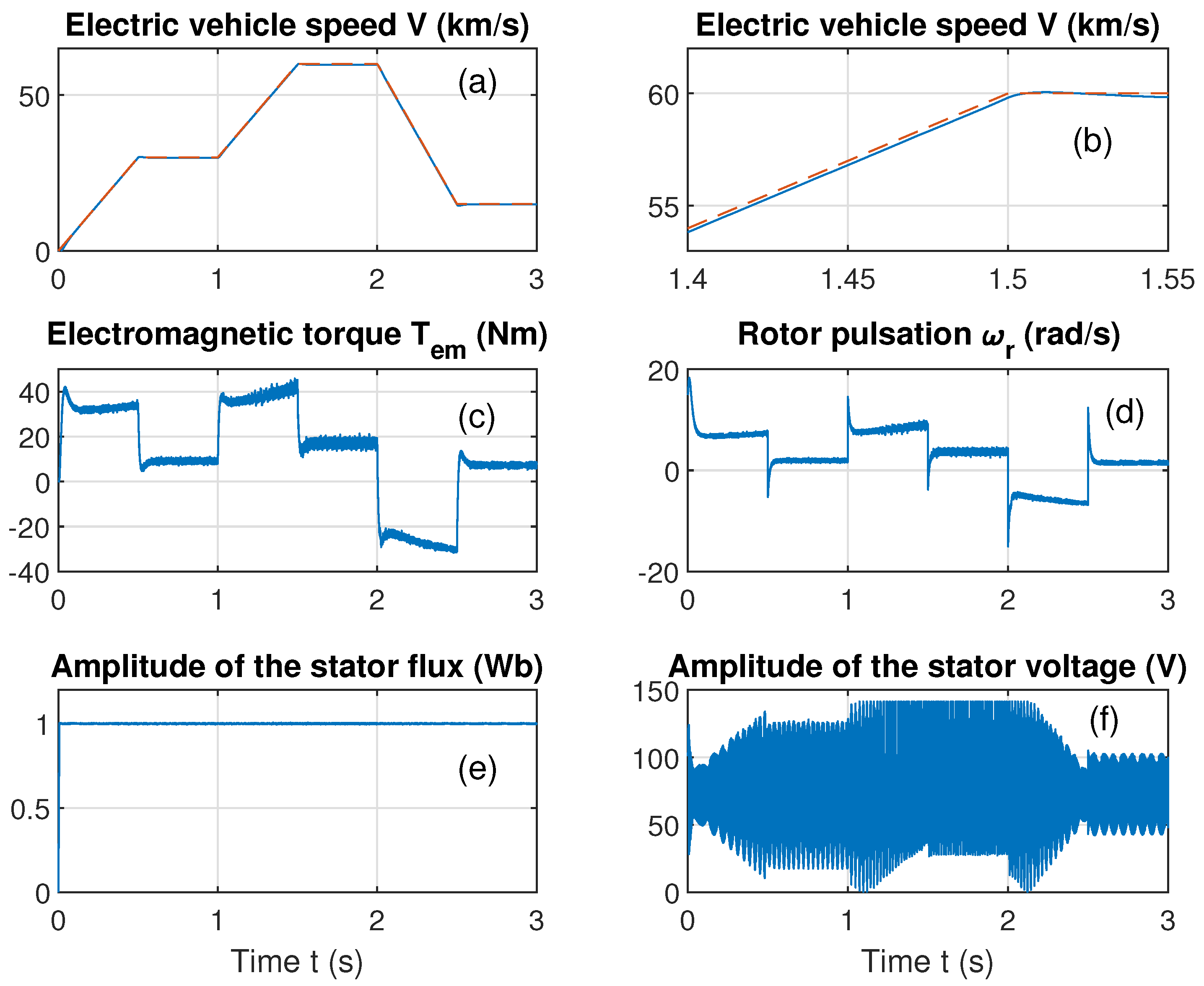
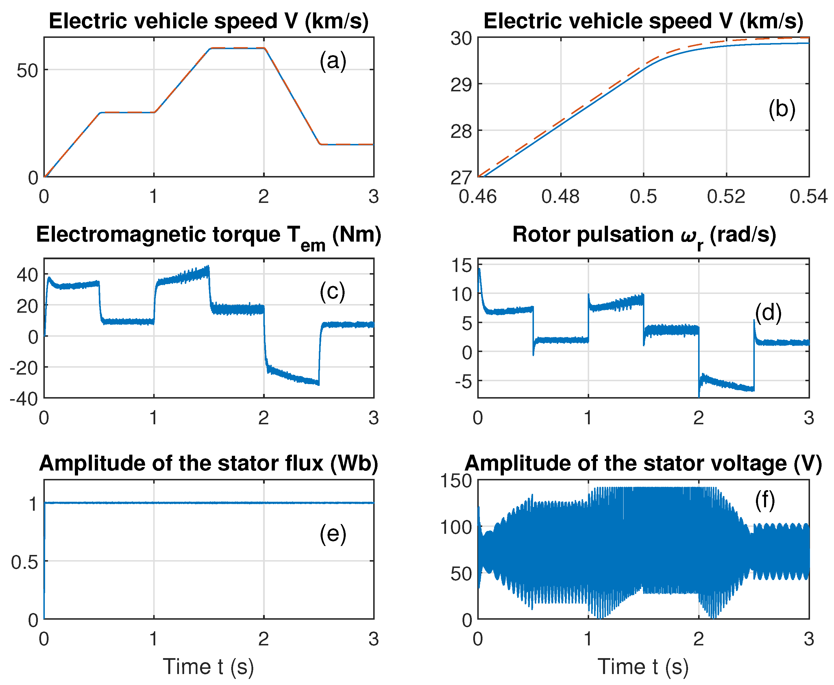
4.2. First Scenario
4.3. Second Scenario
4.4. Third Scenario
5. Conclusions
Author Contributions
Funding
Data Availability Statement
Acknowledgments
Conflicts of Interest
References
- Salahshour, S.; Ahmadian, A.; Senu, N.; Baleanu, D.; Agarwal, P. On analytical solutions of the fractional differential equation with uncertainty: Application to the Basset problem. Entropy 2015, 17, 885–902. [Google Scholar] [CrossRef]
- Gudey, S.; Malla, M.; Jasthi, K.; Gampa, S. Direct torque control of an induction motor using fractional-order sliding mode control technique for quick response and reduced torque ripple. World Electr. Veh. J. 2023, 14, 137. [Google Scholar] [CrossRef]
- Ben Salem, F.; Masmoudi, A. A Comparative Analysis of the Inverter Switching Frequency in Takahashi DTC Strategy. Int. J. Comput. Math. Electr. Electron. Eng. COMPEL 2007, 26, 148–166. [Google Scholar] [CrossRef]
- Sung, G.; Lin, W.; Peng, S. Reduction of Torque and Flux Variations Using Fuzzy Direct Torque Control System in Motor Drive. In Proceedings of the 2013 IEEE International Conference on Systems, Man, and Cybernetics, Manchester, UK, 13–16 October 2013. [Google Scholar]
- Zhao, S.; Yu, H.; Yu, J.; Shan, B. Induction Motor DTC Based on Adaptive SMC and Fuzzy Control. In Proceedings of the 27th Chinese Control and Decision Conference, Qingdao, China, 23–25 May 2015. [Google Scholar]
- Ammar, A.; Bourek, A.; Benakcha, A. Implementation of Robust SVM-DTC for Induction Motor Drive Using Second Order Sliding Mode Control. In Proceedings of the 2016 8th International Conference on Modelling, Identification and Control (ICMIC), Algiers, Algeria, 15–17 November 2016. [Google Scholar]
- Oukaci, A.; Toufouti, R.; Dib, D.; Atarsia, L. Comparison performance between sliding mode control and Nonlinear Control, Application to Induction Motor. Electr. Eng. 2017, 99, 33–45. [Google Scholar] [CrossRef]
- Wang, D.; Yuan, T.; Liu, Z.; Li, Y.; Wang, X.; Tian, W.; Miao, S.; Liu, J. Reduction of Torque and Flux Ripples for Robot Motion Control System Based on SVM-DTC. In Proceedings of the 37th Chinese Control Conference (CCC), Wuhan, China, 25–27 July 2018. [Google Scholar]
- Babes, B.; Boutaghane, A.; Hamouda, N.; Mezaache, M. Design of a Robust Voltage Controller for a DC-DC Buck Converter Using Fractional-Order Terminal Sliding Mode Control Strategy. In Proceedings of the International Conference on Advanced Electrical Engineering, Algiers, Algeria, 19–21 November 2019. [Google Scholar]
- Young, K.D.; Utkin, V.I.; Ozguner, U. A control engineer’s, guide to sliding mode control. IEEE Trans. Control Syst. Technol. 1999, 7, 328–342. [Google Scholar] [CrossRef]
- Lee, K.B.; Bae, C.H.; Blaabjerg, F. An improved DTCSVM method for matrix converter drives using a deadbeat scheme. Int. J. Electron. 2006, 93, 737–753. [Google Scholar] [CrossRef]
- Adamidis, G.; Koutsogiannis, Z.; Vagdatis, P. Investigation of the performance of a variable-speed drive using direct torque control with space vector modulation. Elect. Power Compon. Syst. 2011, 39, 1227–1243. [Google Scholar] [CrossRef]
- Patil, U.V.; Suryawanshi, H.M.; Renge, M.M. Torque ripple minimisation in direct torque control induction motor drive using space vector controlled diode-clamped multi-level invertor. Elect. Power Compon. Syst. 2012, 40, 792–806. [Google Scholar] [CrossRef]
- Nosheen, T.; Ali, A.; Chaudhry, M.U.; Nazarenko, D.; Shaikh, I.u.H.; Bolshev, V.; Iqbal, M.M.; Khalid, S.; Panchenko, V. A Fractional Order Controller for Sensorless Speed Control of an Induction Motor. Energies 2023, 16, 1901. [Google Scholar] [CrossRef]
- Adigintla, S.; Aware, M.V. Robust Fractional Order Speed Controllers for Induction Motor Under Parameter Variations and Low Speed Operating Regions. IEEE Trans. Circuits Syst. II Express Briefs 2023, 70, 1119–1123. [Google Scholar] [CrossRef]
- Ben Salem, F. Winding Fault Diagnosis of Permanent Magnet Synchronous Motor-Based DTC-SVM dedicated to Electric Vehicle Applications. In Autonomous Vehicle and Smart Traffic; IntechOpen: London, UK, 2020. [Google Scholar]
- Bingi, K.; Rajanarayan Prusty, B.; Pal Singh, A. A Review on Fractional-Order Modelling and Control of Robotic Manipulators. Fractal Fract. 2023, 7, 77. [Google Scholar] [CrossRef]
- Duarte-Mermoud, M.A.; Aguila-Camacho, N.; Gallegos, J.A.; Castro-Linares, R. Using general quadratic Lyapunov functions to prove Lyapunov uniform stability for fractional order systems. Commun. Nonlinear Sci. Numer. Simul. 2015, 22, 650–659. [Google Scholar] [CrossRef]
- Aguila-Camacho, N.; Duarte-Mermoud, M.A.; Gallegos, J.A. Lyapunov functions for fractional order systems. Commun. Nonlinear Sci. Numer. Simul. 2014, 19, 2951–2957. [Google Scholar] [CrossRef]
- Sabatier, J.; Lanusse, P.; Melchior, P.; Oustaloup, A. Fractional Order Differentiation and Robust Control Design: CRONE, H-Infinity and Motion Control; Springer: Dordrecht, The Netherlands, 2015. [Google Scholar]
- Yousfi, N.; Melchior, P.; Rekik, C.; Derbel, N.; Oustaloup, A. Path tracking design based on Davidson–Cole prefilter using a centralized CRONE controller applied to multivariable systems. Nonlinear Dyn. 2012, 71, 701–712. [Google Scholar] [CrossRef]
- Li, Y.; Chen, Y.; Podlubny, I. Stability of fractional-order nonlinear dynamic systems: Lyapunov direct method and generalized Mittag Leffler stability. Comput. Math. Appl. 2010, 59, 1810–1821. [Google Scholar] [CrossRef]
- Qing, W.; Pan, B.; Hou, Y.; Lu, S.; Zhang, W. Fractional-Order Sliding Mode Control Method for a Class of Integer-Order Nonlinear Systems. Aerospace 2022, 9, 616. [Google Scholar] [CrossRef]
- Derbel, N.; Zhu, Q. Modeling, Identification and Control Methods in Renewable Energy Systems; Springer: Singapore, 2019. [Google Scholar]
- Ben Salem, F.; Derbel, N. Direct Torque Control of Induction Motors Based on Discrete Space Vector Modulation Using Adaptive Sliding Mode Control. Electr. Power Components Syst. EPCS 2014, 42, 1598–1610. [Google Scholar] [CrossRef]
- Ben Salem, F.; Derbel, N. Second-order Sliding-mode Control Approaches to Improve Low-speed Operation of Induction Machine under Direct Torque Control. Electr. Power Components Syst. EPCS 2016, 44, 1969–1980. [Google Scholar] [CrossRef]
- Ben Salem, F.; Derbel, N. DTC-SVM-Based Sliding Mode Controllers with Load Torque Estimators for Induction Motor Drives. In Applications of Sliding Mode Control, Studies in Systems, Decision and Control; Springer Science and Business Media: Singapore, 2017; Chapter 14; pp. 269–297. [Google Scholar]


| mH | ||
| mH | kg/m2 |
| m | m2 |
| kg | |
| G = 0.9 | kg/m3 |
| 0.0016 | 0.0021 | 0.0066 |
| Time Zone 1 | 0.0482 | 0.0613 | 0.2267 |
| Time Zone 2 | 0.0490 | 0.0611 | 0.2492 |
| Time Zone 3 | 0.0832 | 0.1020 | 0.2631 |
| Time Zone 1 | Time Zone 2 | Time Zone 3 | |
|---|---|---|---|
| THD | 0.0141 | 0.0151 | 0.0047 |
Disclaimer/Publisher’s Note: The statements, opinions and data contained in all publications are solely those of the individual author(s) and contributor(s) and not of MDPI and/or the editor(s). MDPI and/or the editor(s) disclaim responsibility for any injury to people or property resulting from any ideas, methods, instructions or products referred to in the content. |
© 2024 by the authors. Licensee MDPI, Basel, Switzerland. This article is an open access article distributed under the terms and conditions of the Creative Commons Attribution (CC BY) license (https://creativecommons.org/licenses/by/4.0/).
Share and Cite
Ben Salem, F.; Almousa, M.T.; Derbel, N. Enhanced Control Technique for Induction Motor Drives in Electric Vehicles: A Fractional-Order Sliding Mode Approach with DTC-SVM. Energies 2024, 17, 4340. https://doi.org/10.3390/en17174340
Ben Salem F, Almousa MT, Derbel N. Enhanced Control Technique for Induction Motor Drives in Electric Vehicles: A Fractional-Order Sliding Mode Approach with DTC-SVM. Energies. 2024; 17(17):4340. https://doi.org/10.3390/en17174340
Chicago/Turabian StyleBen Salem, Fatma, Motab Turki Almousa, and Nabil Derbel. 2024. "Enhanced Control Technique for Induction Motor Drives in Electric Vehicles: A Fractional-Order Sliding Mode Approach with DTC-SVM" Energies 17, no. 17: 4340. https://doi.org/10.3390/en17174340
APA StyleBen Salem, F., Almousa, M. T., & Derbel, N. (2024). Enhanced Control Technique for Induction Motor Drives in Electric Vehicles: A Fractional-Order Sliding Mode Approach with DTC-SVM. Energies, 17(17), 4340. https://doi.org/10.3390/en17174340