Predicting Industrial Electricity Consumption Using Industry–Geography Relationships: A Graph-Based Machine Learning Approach

Abstract

Accurately predicting industrial electricity consumption is of paramount importance for optimizing energy management and operational efficiency. Traditional forecasting approaches face significant challenges in capturing the complex factors influencing industrial electricity consumption, often due to the inadequate representation of correlations, thus limiting their predictive capabilities. To overcome these limitations, we propose a novel graph-based forecasting model termed Industry–Geography Time Series Forecasting Model (IG-TFM). Our approach leverages historical electricity consumption data and geographical information relevant to similar industries to construct an industry–geography relationship graph. This graph serves as the foundation of a comprehensive network that encompasses all industries of interest, allowing us to identify sectors closely associated with the target industry. The structured graph data are then processed within a graph convolutional neural network framework, which effectively captures the impact of geographical location, industry similarities, and inter-industry relationships on electricity consumption patterns. Utilizing this enriched representation, we develop our IG-TFM for accurate time series forecasting of industrial electricity consumption. Experiments conducted on real-world data, including 31 industries across 9 cities in a southern province of China, demonstrate the significant advantages of our proposed method across key performance indicators such as the Mean Absolute Error (MAE), Root Mean Squared Error (RMSE), and Mean Absolute Percentage Error (MAPE). These findings underscore the importance and efficacy of employing complex networks to encode sequence-related information, thereby substantially improving prediction accuracy in industrial electricity consumption forecasting.

1. Introduction

Electricity consumption forecast is a prediction of future electricity demand in a certain city, industry, or region. In modern society, with the construction of new energy power stations and the growth of power demand, the management of power systems has become more and more complex, bringing new challenges to power consumption forecasting. The accurate prediction of electricity consumption can effectively improve the consumption rate of new energy power and reduce carbon emissions. It is related to the reliability and efficiency of the energy supply and has important research significance and application value [1].

The industry daily electricity consumption forecast studied in this article is essentially a sub-problem of the time series forecast problem. Traditional research methods can be divided into statistics-based methods and machine learning-based methods. Forecasting methods based on traditional statistical models, such as the autoregressive moving average model (ARMA), autoregressive integrated moving average model (ARIMA), etc., have strong robustness and interpretability, but they rely on the assumption of data stationarity, so the forecast objects are generally monthly data. Compared with statistical methods, methods based on traditional machine learning have better nonlinear fitting capabilities and improve prediction accuracy. However, they often need to be combined with feature engineering and rely more on expert experience [2]. With the development of deep learning, Long Short-Term Memory (LSTM) [3,4] has been widely used in time series prediction problems and has achieved remarkable results. However, LSTM only studies a single time series data. For multiple time series data that are related to each other, it is difficult to achieve effective utilization of the data. The DeepAR [5] model based on autoregressive recursive networks can learn a global model from time series and predict the probability distribution of the target sequence. However, DeepAR can only learn univariate distribution. For multivariable multiple time series prediction problems, some works use the copula model to model multivariable distribution [6,7]. Although the above-mentioned multiple time series prediction works make use of related data, the relationship between the sequences is still implicit, and the impact of each related sequence on the target sequence is not distinguished. Although there are Recurrent Neural Networks (RNNs) based on the attention mechanism to capture this influence relationship [8], the limitations of the recurrent neural network itself cannot effectively handle long-term dependencies [9].

For industry electricity consumption, since there must be certain interrelationships between industries [10], and these relationships have a significant impact on industry electricity consumption [11], these influencing factors can be used to improve the predictive ability of the model. In the field of complex network research, the analysis of regional electricity consumption shows that there are important network structural characteristics among them, and based on this, the dynamic effect on electricity intensity can be verified [12]. By constructing a complex network based on industrial electricity consumption in Shanghai, the prediction accuracy of the sequence was improved [13]. How to combine complex network research methods with deep learning to provide an effective and reliable theoretical basis for deep learning, thereby improving the predictive ability of deep learning models, deserves further study.

With the development of the Graph Neural Networks (GNNs) [14], research on applying them to multiple time series forecasting continues to emerge [15]. Graph Convolutional Networks (GCNs) [16] have achieved great success in many tasks by virtue of their effective processing of complex nonlinear relationships between entities in the network. The GC-LSTM [17] that combines the GCN and LSTM uses the correlation between entities to achieve better prediction results than the single LSTM model. However, the graph neural network model requires manual input of the adjacency matrix, that is, the association matrix between entities. This often does not exist for most time series data, so graph neural network models are often used in time series prediction problems with fixed geographical location information such as traffic prediction [18] and air quality prediction [19]. In order to improve prediction accuracy, researchers have developed many methods to obtain more effective graph structures. For example, dynamic spatial–temporal graph convolutional neural networks (DGCNNs) [20] design a dynamic matrix estimator to capture spatial changes, the spatial temporal graph neural network (STGNN) [21] offers a learnable positional attention mechanism to capture spatial and temporal dependencies, and the adaptive spatial–temporal transformer graph network (ASTTGN) [22] captures spatiotemporal relationships through adaptive spatiotemporal transformers. In order to model the relationship network between multiple time series, the multivariate time graph neural network (MTGNN) [23] has been proposed. This method can automatically learn the one-way relationship between variables and use variables as nodes to generate an adjacency matrix for training and prediction.

This paper addresses the problem of predicting daily electricity consumption data for various industries. Due to the interactions between industries, effectively utilizing these relationships can significantly improve the accuracy of industrial electricity consumption predictions. However, the influence relationships between industries are not explicitly expressed. To address this, we constructed an industry–geography graph based on industry electricity consumption data and geographical location information. Using the complex network built from the historical electricity consumption data of all industries, we identified relevant industries and used this information to construct graph-structured data. This data were then fed into a graph convolutional network (GCN) to capture the impact of geography, the same industry, and related industries on the electricity consumption of the target industry. Finally, an LSTM model was utilized to capture time dependence. We call this model the Industry–Geography Time Series Forecasting Model (IG-TFM). The innovation of the IG-TFM model lies in its comprehensive consideration of geographical relationships and the historical data of industries. By using a GCN to effectively mine the potential relationships between industries and integrating this with LSTM, the model fully captures the dynamic changes in time series data. Experimental results demonstrate that the accuracy is significantly improved compared to commonly used time series models. This research not only provides more accurate predictions of electricity consumption for specific industries but also offers a scientific basis for power supply planning and load management, further advancing the development of smart grids and the optimization of power systems.

2. Problem Formulation

The industry electricity consumption time series forecast we studied is based on the historical daily electricity consumption data of 31 manufacturing categories in nine cities in a province in southern China. The data span from 1 January 2020 to 29 January 2023; they are denoted as $\mathbf{D}=\{{\mathbf{X}}_1,{\mathbf{X}}_2,\cdots ,{\mathbf{X}}_i,\cdots ,{\mathbf{X}}_{N-1},{\mathbf{X}}_N\}$, where $N=9$ represents the number of cities, ${\mathbf{X}}_i\in {\mathbb{N}}^{T\times d}$, T represents the length of historical data, and $d=31+6$ is the electricity consumption data of 31 industries in each city and six related variables. These related variables include maximum temperature, minimum temperature, wind speed, whether it is a holiday, whether it is a weekend, and weather conditions. We use $X_i^t=\{x_{i,1}^t,x_{i,2}^t,\cdots ,x_{i,j}^t,\cdots ,x_{i,M-1}^t,x_{i,M}^t,x_{i,{\beta }_1}^t,\cdots ,x_{i,{\beta }_6}^t\}$ to denote the historical data for city i at time t, where $M=31$ represents the number of industries, and $x_{i,j}^t$ represents the electricity consumption of industry j in city i at time t, while $x_{\beta }^t$ represents the related variables. Additionally, $X_{i,j}=\{x_{i,j}^1,x_{i,j}^2,\cdots ,x_{i,j}^t,\cdots ,x_{i,j}^{T-1},x_{i,j}^T\}$ signifies the historical electricity consumption data for industry j in city i. Our goal is to predict the future electricity consumption data ${\widehat{Y}}_{i,j}=\{{\widehat{y}}_{i,j}^{T+1},{\widehat{y}}_{i,j}^{T+2},\cdots ,{\widehat{y}}_{i,j}^{T+L}\}$ for a specified city and industry given the historical data $\mathbf{D}$, where L represents the length of the future electricity consumption data to be predicted.

Given a graph $G=(V,E)$, V is the node set of the graph, and the nodes represent the entities in the graph; E is the edge set in the graph, which is used to represent the connection relationship between entities. For a network/graph, we often use the adjacency matrix A to represent it. For example, when $A_{i,j}=1$, it indicates that there is an edge between nodes i and j, that is, there is a connection relationship between entities i and j.

3. Method

Since there are certain common trends among the same industry in various cities, in order to depict and utilize this relationship, we constructed a relationship graph of the same industry in various cities based on the historical data of the same industry and location information of various cities, which is represented by the adjacency matrix A. In addition to the same industry, related industries will also have an impact on the target industry. In order to use this influence relationship to improve the prediction accuracy, we built a complex network based on all industry historical data, and we obtained the industries related to the predicted industry. Together with the adjacency matrix A, these related industry data can use the GCN model to capture the influence relationships of geography, the same industry, and related industries related to the target industry so as to obtain a better representation, which we fed to LSTM for time series prediction. The overall framework is shown in Figure 1.

3.1. Industry Geography Relationship Graph

First, based on the historical electricity consumption data of the same industry in various cities, we calculated the correlation coefficient between the two to generate the industry correlation matrix $A_1$. Considering that industry relationships are related to geographical location, we generated a correlation matrix $A_2$ based on the geographical location of each city. Finally, an industry geographic relationship matrix was constructed as follows:

$$\begin{array}{c}\hfill A=p{A}_1+q{A}_2,\end{array}$$

(1)

where $p,q$ are the parameters to be learned. By adjusting the weights during learning, the influence relationship between the same industry in various cities and cities can be accurately captured. The industry geographic relationship matrix A was used in different GCN layers and was shared between different layers.

3.1.1. Industry Relationship Graph

We used the Pearson correlation coefficient to calculate the correlations between specified industries in the nine cities as follows:

$$\begin{array}{c}\hfill {\rho }_{ij}(X_{i,·},X_{j,·})={\displaystyle \frac{{\displaystyle \sum _{t=1}^T}(x_{i,·}^t-{\overline{X}}_{i,·})(x_{j,·}^t-{\overline{X}}_{j,·})}{\sqrt{{\displaystyle \sum _{t=1}^T}{(x_{i,·}^t-{\overline{X}}_{i,·})}^2}\sqrt{{\displaystyle \sum _{t=1}^T}{(x_{j,·}^t-{\overline{X}}_{j,·})}^2}}},\end{array}$$

(2)

where $\rho \in [-1,1]$; $\rho =1$ indicates complete positive correlation between a particular industry in city i and j, and $\rho =-1$ indicates complete negative correlation. $X_{i,·},X_{j,·}$ represent the historical electricity consumption data of a particular industry in cities i and j, respectively. ${\overline{X}}_{i,·}={\sum }_{t=1}^T{x}_{i,·}^t/T,{\overline{X}}_{j,·}={\sum }_{t=1}^T{x}_{j,·}^t/T$. This correlation coefficient allowed us to construct an industry relationship matrix, which characterizes the correlations between industries in the same cities.

$$\begin{array}{c}\hfill A_{1(i,j)}=\left\{\begin{array}{c}{\rho }_{i,j},i\ne j\hfill \\ 1,i=j\hfill \end{array}.\right.\end{array}$$

(3)

3.1.2. Geographical Relationship Graph

Since there is a certain influence between the industry and the same industry in neighboring cities, in order to take this influencing factor into consideration, we constructed an industry distance graph based on the geographical location information of each city:

$$\begin{array}{c}\hfill A_{2(i,j)}=\left\{\begin{array}{c}{\displaystyle \frac{1}{d_{ij}}},i\ne j\mathrm{and}{d}_{ij}<R\hfill \\ 0,\mathrm{else}\hfill \end{array},\right.\end{array}$$

(4)

where $d_{i,j}$ represents the distance between city i and j centers, and $R=125\mathrm{km}$, indicating that two industries are considered to have an impact on each other only within a distance of R.

3.2. Extract Related Industries

Since related industries will also have an impact on the target industry, in order to take advantage of this influence relationship, we selected related industries by building a complex network. First, for all industries in the same city, based on the historical data of each industry, we used the Pearson correlation coefficient to calculate the correlation between each industry:

$$\begin{array}{c}\hfill {\rho }_{mn}(X_{·,m},X_{·,n})={\displaystyle \frac{{\displaystyle \sum _{t=1}^T}(x_{·,m}^t-{\overline{X}}_{·,m})(x_{·,n}^t-{\overline{X}}_{·,n})}{\sqrt{{\displaystyle \sum _{t=1}^T}{(x_{·,m}^t-{\overline{X}}_{·,m})}^2}\sqrt{{\displaystyle \sum _{t=1}^T}{(x_n^t-{\overline{X}}_{·,n})}^2}}},\end{array}$$

(5)

where $X_{·,m},X_{·,n}$ represent the historical electricity consumption data for industry $m,n$ in the city, respectively. ${\overline{X}}_{·,m}={\sum }_{t=1}^T{x}_{·,m}^t/T,{\overline{X}}_{·,n}={\sum }_{t=1}^T{x}_{·,n}^t/T$. Based on this coefficient, we calculated the distance between two time series as follows:

$$\begin{array}{c}\hfill d_{m,n}=\sqrt{2·(1-{\rho }_{m,n})}.\end{array}$$

(6)

Based on this distance, an industry distance matrix can be generated, which represents the distance between the industries represented by each node in the network. However, the network built based on this distance matrix is almost fully connected and has a large number of redundant edges. In order to extract key information from it, we used Prim’s algorithm [24] to prune the original network to obtain the minimum spanning tree (MST), and we then used the method in [13,25] to construct the plane maximum filter graph (PMFG); this method is widely used in economics and finance to analyze the relationship between network entities. Compared to the MST, the PMFG has more edges and higher connectivity. Each of these nodes is connected to at least two other nodes, which means that each industry will have at least two related industries. So, it can retain more effective information regarding the distance matrix and the simplicity of the MST at the same time.

We hoped to further discover industries that have potential relationships with the target industry from the network structure of the PMFG, so we used the Louvain algorithm [26] to classify nodes in the PMFG as communities. This algorithm performs node clustering based on modularity and has a higher robustness. The calculation formula for modularity is as follows:

$$\begin{array}{c}\hfill Q={\displaystyle \frac{1}{2K}}\sum _{m,n}\left(d_{m,n}-{\displaystyle \frac{k_m{k}_n}{2K}}\right)\delta (c_m,c_n),\end{array}$$

(7)

where $K={\Sigma }_{mn}{d}_{m,n}/2,k_m={\Sigma }_n{d}_{m,n},\delta (c_m,c_n)\in \{0,1\}$, $\delta (c_m,c_n)=1$ if $c_m=c_n$, $c_m$ represents the community that node m is assigned to. During the iterative process, each node in the graph is initially treated as a community. We attempt to add a node to its neighbor’s community and calculate the increment in modularity index $\mathsf{\Delta }Q$, and we choose the neighboring community that maximizes $\mathsf{\Delta }Q$. The calculation formula for the increment in modularity index $\mathsf{\Delta }Q$ is as follows:

$$\begin{array}{c}\hfill \mathsf{\Delta }Q={\displaystyle \frac{k_{m,\mathrm{in}}}{2K}}-{\displaystyle \frac{{\sum }_{\mathrm{tot}}{k}_m}{2K^2}},\end{array}$$

(8)

where $k_{m,\mathrm{in}}$ is the sum of the weights of the links from i to nodes in community, ${\sum }_{\mathrm{tot}}$ is the sum of the weights of the links incident to nodes in community. The iteration ends when $\mathsf{\Delta }Q$ is smaller than a certain threshold a.

The community classification results are shown in Figure 2. For a considerable number of nodes, although there are many nodes connected to them, the results of modularity classification indicate that they do not belong to the same category as the connected nodes. This classification result further helps us select related industries of target industry j, which are denoted as $\mathcal{R}\left(j\right)$.

3.3. Graph Convolutional Networks

The graph convolutional network (GCN) updates the node representation by aggregating the information of the neighboring nodes of each node, which can better characterize the complex nonlinear relationships between nodes in the network. Therefore, it has been widely used in tasks related to graph structure data analysis. Given a graph $G=(V,E)$, when the model is trained, the update process of node representation is as follows:

$$\begin{array}{c}\hfill x_i^{l+1}=\sigma \left(\sum _{j\in {\mathcal{N}}_i}{\displaystyle \frac{1}{c_{ij}}}{x}_j^l{w}^l+b^l\right),\end{array}$$

(9)

where $x_i^{l+1}$ represents the representation of node i after passing through the lth layer of the neural networks, $\sigma$ is the activation function, ${\mathcal{N}}_i$ represents the neighborhood nodes of node i, $c_{ij}=\sqrt{\mathrm{deg}\left(v_i\right)}\sqrt{\mathrm{deg}\left(v_j\right)}$, $\mathrm{deg}\left(\mathrm{i}\right)$ is the degree of node i, $w^l$ is the weight of the lth layer neural network, and $b^l$ is the bias term of the lth layer.

3.4. LSTM

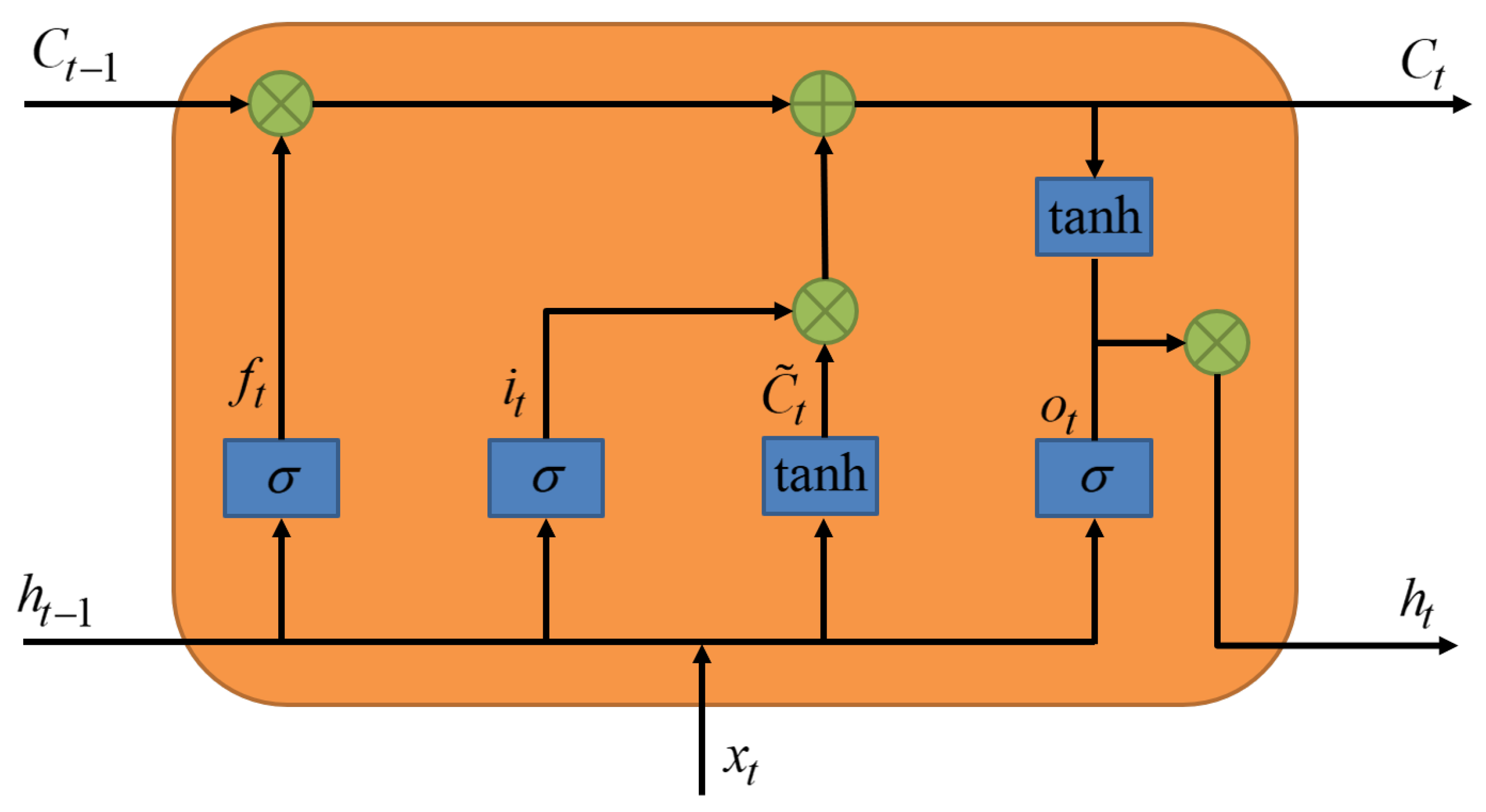
RNNs require the current hidden state, as well as the previous time step’s hidden state in each hidden layer, to effectively handle sequential data. However, RNNs suffer from vanishing gradient and exploding gradient problems and struggle to capture long-term dependencies. LSTM addresses these issues by adding three gate units $i_t,f_t,o_t$ to control information flow, enabling the model to remember and forget information for both short and long time spans. The structure of an individual LSTM cell is as shown in Figure 3.

The formula of the forward propagation process of LSTM is as follows:

$$\begin{array}{cc}\hfill i_t& =\sigma (W_i·[h_{t-1},x_t]+b_i),\hfill \end{array}$$

(10)

$$\begin{array}{cc}\hfill f_t& =\sigma (W_f·[h_{t-1},x_t]+b_f),\hfill \end{array}$$

(11)

$$\begin{array}{cc}\hfill o_t& =\sigma (W_o·[h_{t-1},x_t]+b_o),\hfill \end{array}$$

(12)

$$\begin{array}{cc}\hfill {\tilde{C}}_t& =tanh(W_c·[h_{t-1},x_t]+b_c),\hfill \end{array}$$

(13)

$$\begin{array}{cc}\hfill C_t& =f_t\odot C_{t-1}+i_t\odot {\tilde{C}}_t,\hfill \end{array}$$

(14)

$$\begin{array}{cc}\hfill h_t& =o_t\odot tanh\left(C_t\right),\hfill \end{array}$$

(15)

where $i_t,f_t,o_t$ are the input gate, forget gate, and output gate, respectively. These gates are binary (0 or 1) and control whether to let the information flow through. $C_t$ represents the cell that transfers information from one time step to another, allowing LSTM to avoid the vanishing gradient problem. For a single time step, the current state $x_t$ enters the cell, and the previous hidden state $h_{t-1}$ enters the forget gate $f_t$. If the output is 0, the information $C_t$ from the previous time step is forgotten. The input gate $i_t$ determines whether the current state enters the cell. Finally, the output gate $o_t$ decides the output of the hidden state $h_t$ in this layer.

3.5. Model Architecture

As shown in Figure 1, we constructed industry–geography relationship graphs A based on historical data of the same industry within geographic information, obtaining related industries $\mathcal{R}\left(j\right)$ by building the complex network. Based on this, we constructed the graph structure data $G=(V,E)$, where the node $v_i$ in set V represents the city, and the edge set E represents the connections between nodes. The features of node $v_i$ are $(X_{i,j},X_{i,\mathcal{R}\left(j\right)},x_{i,{\beta }_1},\cdots ,x_{i,{\beta }_6})$. This graph structure data are fed into the GCN model to capture the effects of geography, the same industry, and related industries on the target industry j; the output is the electricity consumption data of the target industries in all cities. Select the data of any city as the input of the LSTM model, which has excellent capabilities for handling sequential data and is used for forecasting future industry electricity consumption.

4. Experimental Studies

4.1. Data

The data were calculated based on the power consumption collection system of a provincial electric power company of the State Grid Corporation of China. The electricity consumption collection system includes collection terminals and collection platforms for 20 million users in the province. The next day, the frozen display at 24:00 of the previous day will be returned. The difference from the frozen display of the previous day and according to certain calculation logic will be used to obtain the daily electricity consumption of each household. And based on the Oracle database, the user profile data were matched, the daily power data are obtained by summarizing the regions and power consumption categories, and the time series is obtained by arranging the data in order.

4.2. Experimental Setting

We divided the dataset into three parts according to the time length, with the first 60% as the training set, 20% as the validation set, and the last 20% as the test set. The learning rate was set to 0.001, the loss function was defined as the mean absolute error (MAE), the maximum training cycle was 1000, an early stopping mechanism was set to retain the best parameters obtained during training, and the batch size was set to 15.

To verify the performance of our proposed model in industry electricity consumption prediction, we compared it with the following classic prediction models: recurrent neural networks (RNNs), the gated recurrent unit (GRU) [27], the graph convolutional neural network, long short-term memory(GC-LSTM) [17], and Multilayer Perceptron (MLP), as well as LSTM(1), which only used the target industry data $X_j$ for training, while LSTM(2) used both the target industry information $X_j$ and the related industry information $\mathcal{R}\left(j\right)$. For the Industry–Geography Time Series Forecasting Model (IG-TFM) we proposed, we set up ablation experiments in four cases: Model 1 uses industry geographic information A and related industry information $\mathcal{R}\left(j\right)$—denoted as $\mathrm{IG}-\mathrm{TFM}(A,X_j,X_{\mathcal{R}\left(j\right)})$; Model 2 uses city geographic information A—denoted as $\mathrm{IG}-\mathrm{TFM}(A,X_j)$; Model 3 uses related industry information $\mathcal{R}\left(j\right)$—denoted as $\mathrm{IG}-\mathrm{TFM}(X_j,X_{\mathcal{R}\left(j\right)})$; and Model 4 does not use A and $\mathcal{R}\left(j\right)$, but only relies on the target industry data $X_j$ itself for prediction—denoted as $\mathrm{IG}-\mathrm{TFM}\left(X_j\right)$. Except for the different information used, the number of network layers and the number of neurons in each layer were the same. The above ablation experiment setting is shown in

Table 1. Ablation experiment setup.

Model	IG-TFM	Information Used
Model 1	$\mathrm{IG}-\mathrm{TFM}(A,X_j,X_{\mathcal{R}\left(j\right)})$	$A,X_j,X_{\mathcal{R}\left(j\right)}$
Model 2	$\mathrm{IG}-\mathrm{TFM}(A,X_j)$	$A,X_j$
Model 3	$\mathrm{IG}-\mathrm{TFM}(X_j,X_{\mathcal{R}\left(j\right)})$	$X_j,X_{\mathcal{R}\left(j\right)}$
Model 4	$\mathrm{IG}-\mathrm{TFM}\left(X_j\right)$	$X_j$

.

In fact, since our adjacency matrix is a linear combination of two matrices, our model can be seen as a generalization of the GC-LSTM model. When the coefficient of one of the matrices is zero, Model 2 can be considered equivalent to the GC-LSTM. For the convenience of observation and comparison, GC-LSTM in the following text is represented by Model 2.

To measure model performance from multiple perspectives, we used three metrics: mean absolute error (MAE), root mean square error (RMSE), and mean absolute percentage error (MAPE):

$$\begin{array}{cc}\hfill \mathrm{MAE}& ={\displaystyle \frac{1}{L}}\left(\sum _{i=1}^L|y_i-{\widehat{y}}_i|\right),\hfill \end{array}$$

(16)

$$\begin{array}{cc}\hfill \mathrm{RMSE}& =\sqrt{{\displaystyle \frac{1}{L}}\sum _{i=1}^L{(y_i-{\widehat{y}}_i)}^2},\hfill \end{array}$$

(17)

$$\begin{array}{cc}\hfill \mathrm{MAPE}& ={\displaystyle \frac{1}{L}}\sum _{i=1}^L{\displaystyle \frac{|y_i-{\widehat{y}}_i|}{y_i}},\hfill \end{array}$$

(18)

where $y_i,{\widehat{y}}_i$ represent the true and predicted values, respectively.

4.3. Main Results

The experimental results of industry 1 are shown in

Table 2. Experimental results of industry 1.

City	Metric	RNN	GRU	MLP	LSTM(1)	LSTM(2)	Model 1	Model 2	Model 3	Model 4
City 1	MAE	3.83$\times {10}^{-4}$	3.72$\times {10}^{-4}$	3.82$\times {10}^{-4}$	4.10$\times {10}^{-4}$	4.08$\times {10}^{-4}$	2.77$\times {10}^{-4}$	4.22$\times {10}^{-4}$	3.08$\times {10}^{-4}$	3.23$\times {10}^{-4}$
	RMSE	4.96$\times {10}^{-4}$	4.90$\times {10}^{-4}$	5.05$\times {10}^{-4}$	5.35$\times {10}^{-4}$	5.21$\times {10}^{-4}$	3.72$\times {10}^{-4}$	5.49$\times {10}^{-4}$	3.97$\times {10}^{-4}$	4.26$\times {10}^{-4}$
	MAPE	9.89$\times {10}^{-2}$	9.80$\times {10}^{-2}$	1.01$\times {10}^{-1}$	1.06$\times {10}^{-1}$	1.03$\times {10}^{-1}$	6.94$\times {10}^{-2}$	1.05$\times {10}^{-1}$	7.68$\times {10}^{-2}$	8.18$\times {10}^{-2}$
City 2	MAE	7.17$\times {10}^{-4}$	8.07$\times {10}^{-4}$	8.78$\times {10}^{-4}$	7.77$\times {10}^{-4}$	8.21$\times {10}^{-4}$	6.10$\times {10}^{-4}$	9.26$\times {10}^{-4}$	8.28$\times {10}^{-4}$	7.60$\times {10}^{-4}$
	RMSE	9.91$\times {10}^{-4}$	1.07$\times {10}^{-3}$	1.11$\times {10}^{-3}$	1.03$\times {10}^{-3}$	1.02$\times {10}^{-3}$	8.02$\times {10}^{-4}$	1.19$\times {10}^{-3}$	1.03$\times {10}^{-3}$	1.00$\times {10}^{-3}$
	MAPE	1.07$\times {10}^{-1}$	1.21$\times {10}^{-1}$	1.25$\times {10}^{-1}$	1.07$\times {10}^{-1}$	1.11$\times {10}^{-1}$	7.85$\times {10}^{-2}$	1.21$\times {10}^{-1}$	1.07$\times {10}^{-1}$	1.02$\times {10}^{-1}$
City 3	MAE	5.27$\times {10}^{-4}$	5.09$\times {10}^{-4}$	5.15$\times {10}^{-4}$	5.02$\times {10}^{-4}$	4.46$\times {10}^{-4}$	4.37$\times {10}^{-4}$	4.66$\times {10}^{-4}$	5.08$\times {10}^{-4}$	5.21$\times {10}^{-4}$
	RMSE	7.48$\times {10}^{-4}$	7.23$\times {10}^{-4}$	7.61$\times {10}^{-4}$	7.47$\times {10}^{-4}$	6.31$\times {10}^{-4}$	5.82$\times {10}^{-4}$	6.34$\times {10}^{-4}$	6.57$\times {10}^{-4}$	6.91$\times {10}^{-4}$
	MAPE	1.21$\times {10}^{-1}$	1.15$\times {10}^{-1}$	1.24$\times {10}^{-1}$	9.98$\times {10}^{-2}$	8.37$\times {10}^{-2}$	8.11$\times {10}^{-2}$	8.38$\times {10}^{-2}$	8.82$\times {10}^{-2}$	9.60$\times {10}^{-2}$
City 4	MAE	6.60$\times {10}^{-4}$	6.65$\times {10}^{-4}$	6.83$\times {10}^{-4}$	6.85$\times {10}^{-4}$	8.13$\times {10}^{-4}$	6.08$\times {10}^{-4}$	6.77$\times {10}^{-4}$	8.06$\times {10}^{-4}$	6.21$\times {10}^{-4}$
	RMSE	8.37$\times {10}^{-4}$	8.49$\times {10}^{-4}$	8.83$\times {10}^{-4}$	8.52$\times {10}^{-4}$	1.06$\times {10}^{-3}$	7.66$\times {10}^{-4}$	8.71$\times {10}^{-4}$	9.91$\times {10}^{-4}$	7.84$\times {10}^{-4}$
	MAPE	3.27$\times {10}^{-1}$	3.26$\times {10}^{-1}$	3.30$\times {10}^{-1}$	3.04$\times {10}^{-1}$	2.80$\times {10}^{-1}$	2.32$\times {10}^{-1}$	2.42$\times {10}^{-1}$	2.62$\times {10}^{-1}$	2.35$\times {10}^{-1}$
City 5	MAE	1.13$\times {10}^{-4}$	1.15$\times {10}^{-4}$	1.17$\times {10}^{-4}$	1.22$\times {10}^{-4}$	1.31$\times {10}^{-4}$	1.76$\times {10}^{-4}$	1.83$\times {10}^{-4}$	2.13$\times {10}^{-4}$	1.72$\times {10}^{-4}$
	RMSE	1.52$\times {10}^{-4}$	1.56$\times {10}^{-4}$	1.59$\times {10}^{-4}$	1.55$\times {10}^{-4}$	1.67$\times {10}^{-4}$	2.32$\times {10}^{-4}$	2.67$\times {10}^{-4}$	3.49$\times {10}^{-4}$	2.29$\times {10}^{-4}$
	MAPE	1.59$\times {10}^{-1}$	1.64$\times {10}^{-1}$	1.66$\times {10}^{-1}$	1.66$\times {10}^{-1}$	1.65$\times {10}^{-1}$	1.86$\times {10}^{-1}$	2.22$\times {10}^{-1}$	2.25$\times {10}^{-1}$	1.88$\times {10}^{-1}$
City 6	MAE	2.27$\times {10}^{-4}$	2.18$\times {10}^{-4}$	2.32$\times {10}^{-4}$	2.10$\times {10}^{-4}$	3.06$\times {10}^{-4}$	1.82$\times {10}^{-4}$	2.43$\times {10}^{-4}$	2.71$\times {10}^{-4}$	2.20$\times {10}^{-4}$
	RMSE	3.25$\times {10}^{-4}$	3.20$\times {10}^{-4}$	3.31$\times {10}^{-4}$	2.86$\times {10}^{-4}$	4.25$\times {10}^{-4}$	2.48$\times {10}^{-4}$	3.30$\times {10}^{-4}$	4.00$\times {10}^{-4}$	3.18$\times {10}^{-4}$
	MAPE	9.94$\times {10}^{-2}$	9.89$\times {10}^{-2}$	1.02$\times {10}^{-1}$	8.31$\times {10}^{-2}$	1.14$\times {10}^{-1}$	5.73$\times {10}^{-2}$	8.17$\times {10}^{-2}$	9.23$\times {10}^{-2}$	7.49$\times {10}^{-2}$
City 7	MAE	4.72$\times {10}^{-5}$	5.19$\times {10}^{-5}$	4.68$\times {10}^{-5}$	4.96$\times {10}^{-5}$	5.18$\times {10}^{-5}$	5.32$\times {10}^{-5}$	8.68$\times {10}^{-5}$	7.27$\times {10}^{-5}$	6.67$\times {10}^{-5}$
	RMSE	6.64$\times {10}^{-5}$	6.91$\times {10}^{-5}$	6.62$\times {10}^{-5}$	7.10$\times {10}^{-5}$	6.49$\times {10}^{-5}$	6.56$\times {10}^{-5}$	1.19$\times {10}^{-4}$	1.11$\times {10}^{-4}$	8.04$\times {10}^{-5}$
	MAPE	1.11$\times {10}^{-1}$	1.16$\times {10}^{-1}$	1.11$\times {10}^{-1}$	1.18$\times {10}^{-1}$	1.07$\times {10}^{-1}$	9.39$\times {10}^{-2}$	1.75$\times {10}^{-1}$	1.49$\times {10}^{-1}$	1.39$\times {10}^{-1}$
City 8	MAE	1.14$\times {10}^{-4}$	1.13$\times {10}^{-4}$	1.13$\times {10}^{-4}$	1.23$\times {10}^{-4}$	1.46$\times {10}^{-4}$	1.31$\times {10}^{-4}$	1.38$\times {10}^{-4}$	1.35$\times {10}^{-4}$	1.34$\times {10}^{-4}$
	RMSE	1.62$\times {10}^{-4}$	1.63$\times {10}^{-4}$	1.63$\times {10}^{-4}$	1.81$\times {10}^{-4}$	2.10$\times {10}^{-4}$	1.70$\times {10}^{-4}$	1.81$\times {10}^{-4}$	1.75$\times {10}^{-4}$	1.78$\times {10}^{-4}$
	MAPE	1.68$\times {10}^{-1}$	1.73$\times {10}^{-1}$	1.71$\times {10}^{-1}$	2.02$\times {10}^{-1}$	1.52$\times {10}^{-1}$	1.25$\times {10}^{-1}$	1.45$\times {10}^{-1}$	1.39$\times {10}^{-1}$	1.37$\times {10}^{-1}$
City 9	MAE	2.30$\times {10}^{-4}$	2.39$\times {10}^{-4}$	2.42$\times {10}^{-4}$	2.76$\times {10}^{-4}$	2.80$\times {10}^{-4}$	2.56$\times {10}^{-4}$	3.32$\times {10}^{-4}$	2.69$\times {10}^{-4}$	2.27$\times {10}^{-4}$
	RMSE	3.02$\times {10}^{-4}$	3.08$\times {10}^{-4}$	3.14$\times {10}^{-4}$	3.65$\times {10}^{-4}$	3.60$\times {10}^{-4}$	3.24$\times {10}^{-4}$	4.17$\times {10}^{-4}$	3.69$\times {10}^{-4}$	3.05$\times {10}^{-4}$
	MAPE	1.17$\times {10}^{-1}$	1.20$\times {10}^{-1}$	1.23$\times {10}^{-1}$	1.45$\times {10}^{-1}$	1.44$\times {10}^{-1}$	1.08$\times {10}^{-1}$	1.49$\times {10}^{-1}$	1.18$\times {10}^{-1}$	1.05$\times {10}^{-1}$

The best result in each row is bolded.

, and the experimental results of industry 2 are shown in Appendix A 

Table A1. Experimental results of industry 2.

City	Metric	RNN	GRU	MLP	LSTM(1)	LSTM(2)	Model 1	Model 2	Model 3	Model 4
City 1	MAE	3.72$\times {10}^{-4}$	3.84$\times {10}^{-4}$	3.67$\times {10}^{-4}$	8.06$\times {10}^{-5}$	7.52$\times {10}^{-5}$	7.67$\times {10}^{-5}$	1.36$\times {10}^{-4}$	8.99$\times {10}^{-5}$	1.56$\times {10}^{-4}$
	RMSE	4.94$\times {10}^{-4}$	4.97$\times {10}^{-4}$	4.90$\times {10}^{-4}$	1.04$\times {10}^{-4}$	9.94$\times {10}^{-5}$	1.00$\times {10}^{-4}$	1.63$\times {10}^{-4}$	1.12$\times {10}^{-4}$	1.91$\times {10}^{-4}$
	MAPE	9.95$\times {10}^{-2}$	9.84$\times {10}^{-2}$	9.62$\times {10}^{-2}$	1.86$\times {10}^{-1}$	1.69$\times {10}^{-1}$	1.57$\times {10}^{-1}$	2.36$\times {10}^{-1}$	1.74$\times {10}^{-1}$	2.69$\times {10}^{-1}$
City 2	MAE	7.74$\times {10}^{-4}$	7.72$\times {10}^{-4}$	8.83$\times {10}^{-4}$	5.69$\times {10}^{-4}$	5.11$\times {10}^{-4}$	4.16$\times {10}^{-4}$	7.02$\times {10}^{-4}$	7.16$\times {10}^{-4}$	5.37$\times {10}^{-4}$
	RMSE	1.05$\times {10}^{-3}$	1.02$\times {10}^{-3}$	1.11$\times {10}^{-3}$	7.28$\times {10}^{-4}$	7.03$\times {10}^{-4}$	5.43$\times {10}^{-4}$	9.37$\times {10}^{-4}$	8.86$\times {10}^{-4}$	6.91$\times {10}^{-4}$
	MAPE	1.16$\times {10}^{-1}$	1.13$\times {10}^{-1}$	1.24$\times {10}^{-1}$	3.43$\times {10}^{-1}$	3.39$\times {10}^{-1}$	1.40$\times {10}^{-1}$	2.58$\times {10}^{-1}$	2.35$\times {10}^{-1}$	1.93$\times {10}^{-1}$
City 3	MAE	3.75$\times {10}^{-4}$	4.16$\times {10}^{-4}$	3.95$\times {10}^{-4}$	5.18$\times {10}^{-4}$	4.01$\times {10}^{-4}$	4.63$\times {10}^{-4}$	5.09$\times {10}^{-4}$	4.51$\times {10}^{-4}$	5.38$\times {10}^{-4}$
	RMSE	4.99$\times {10}^{-4}$	5.08$\times {10}^{-4}$	4.96$\times {10}^{-4}$	6.23$\times {10}^{-4}$	5.66$\times {10}^{-4}$	6.02$\times {10}^{-4}$	6.63$\times {10}^{-4}$	5.87$\times {10}^{-4}$	6.75$\times {10}^{-4}$
	MAPE	1.98$\times {10}^{-1}$	1.79$\times {10}^{-1}$	2.15$\times {10}^{-1}$	1.67$\times {10}^{-1}$	1.53$\times {10}^{-1}$	1.72$\times {10}^{-1}$	2.15$\times {10}^{-1}$	1.83$\times {10}^{-1}$	2.08$\times {10}^{-1}$
City 4	MAE	6.70$\times {10}^{-4}$	6.74$\times {10}^{-4}$	6.62$\times {10}^{-4}$	3.24$\times {10}^{-4}$	3.14$\times {10}^{-4}$	3.19$\times {10}^{-4}$	5.04$\times {10}^{-4}$	4.60$\times {10}^{-4}$	4.72$\times {10}^{-4}$
	RMSE	8.47$\times {10}^{-4}$	8.43$\times {10}^{-4}$	8.58$\times {10}^{-4}$	4.13$\times {10}^{-4}$	4.28$\times {10}^{-4}$	4.03$\times {10}^{-4}$	5.59$\times {10}^{-4}$	5.15$\times {10}^{-4}$	5.36$\times {10}^{-4}$
	MAPE	3.30$\times {10}^{-1}$	3.27$\times {10}^{-1}$	3.30$\times {10}^{-1}$	3.09$\times {10}^{-1}$	3.55$\times {10}^{-1}$	2.04$\times {10}^{-1}$	2.59$\times {10}^{-1}$	2.37$\times {10}^{-1}$	2.55$\times {10}^{-1}$
City 5	MAE	1.14$\times {10}^{-4}$	1.15$\times {10}^{-4}$	1.13$\times {10}^{-4}$	1.17$\times {10}^{-3}$	1.07$\times {10}^{-3}$	1.13$\times {10}^{-3}$	1.09$\times {10}^{-3}$	1.29$\times {10}^{-3}$	1.22$\times {10}^{-3}$
	RMSE	1.51$\times {10}^{-4}$	1.50$\times {10}^{-4}$	1.53$\times {10}^{-4}$	1.50$\times {10}^{-3}$	1.38$\times {10}^{-3}$	1.45$\times {10}^{-3}$	1.41$\times {10}^{-3}$	1.58$\times {10}^{-3}$	1.62$\times {10}^{-3}$
	MAPE	1.59$\times {10}^{-1}$	1.57$\times {10}^{-1}$	1.59$\times {10}^{-1}$	2.35$\times {10}^{-1}$	2.11$\times {10}^{-1}$	2.25$\times {10}^{-1}$	2.20$\times {10}^{-1}$	2.60$\times {10}^{-1}$	2.79$\times {10}^{-1}$
City 6	MAE	2.24$\times {10}^{-4}$	2.04$\times {10}^{-4}$	2.32$\times {10}^{-4}$	1.78$\times {10}^{-4}$	2.25$\times {10}^{-4}$	1.62$\times {10}^{-4}$	2.53$\times {10}^{-4}$	2.09$\times {10}^{-4}$	2.79$\times {10}^{-4}$
	RMSE	3.21$\times {10}^{-4}$	2.89$\times {10}^{-4}$	3.29$\times {10}^{-4}$	2.91$\times {10}^{-4}$	3.49$\times {10}^{-4}$	2.64$\times {10}^{-4}$	4.29$\times {10}^{-4}$	3.28$\times {10}^{-4}$	4.73$\times {10}^{-4}$
	MAPE	9.71$\times {10}^{-2}$	8.21$\times {10}^{-2}$	1.02$\times {10}^{-1}$	1.15$\times {10}^{-1}$	1.65$\times {10}^{-1}$	9.32$\times {10}^{-2}$	1.57$\times {10}^{-1}$	1.23$\times {10}^{-1}$	1.67$\times {10}^{-1}$
City 7	MAE	7.96$\times {10}^{-4}$	7.84$\times {10}^{-4}$	8.13$\times {10}^{-4}$	1.01$\times {10}^{-3}$	1.04$\times {10}^{-3}$	8.36$\times {10}^{-4}$	1.03$\times {10}^{-3}$	1.04$\times {10}^{-3}$	1.02$\times {10}^{-3}$
	RMSE	1.07$\times {10}^{-3}$	1.05$\times {10}^{-3}$	1.08$\times {10}^{-3}$	1.25$\times {10}^{-3}$	1.26$\times {10}^{-3}$	1.06$\times {10}^{-3}$	1.30$\times {10}^{-3}$	1.33$\times {10}^{-3}$	1.34$\times {10}^{-3}$
	MAPE	3.39$\times {10}^{-1}$	3.38$\times {10}^{-1}$	3.68$\times {10}^{-1}$	3.45$\times {10}^{-1}$	4.06$\times {10}^{-1}$	1.84$\times {10}^{-1}$	2.27$\times {10}^{-1}$	2.26$\times {10}^{-1}$	2.23$\times {10}^{-1}$
City 8	MAE	2.30$\times {10}^{-3}$	2.30$\times {10}^{-3}$	2.32$\times {10}^{-3}$	2.39$\times {10}^{-3}$	2.42$\times {10}^{-3}$	1.66$\times {10}^{-3}$	2.54$\times {10}^{-3}$	2.63$\times {10}^{-3}$	2.46$\times {10}^{-3}$
	RMSE	2.98$\times {10}^{-3}$	2.93$\times {10}^{-3}$	3.02$\times {10}^{-3}$	2.94$\times {10}^{-3}$	3.16$\times {10}^{-3}$	2.06$\times {10}^{-3}$	3.15$\times {10}^{-3}$	3.45$\times {10}^{-3}$	3.10$\times {10}^{-3}$
	MAPE	1.94$\times {10}^{-1}$	1.83$\times {10}^{-1}$	1.95$\times {10}^{-1}$	1.88$\times {10}^{-1}$	1.56$\times {10}^{-1}$	8.87$\times {10}^{-2}$	1.34$\times {10}^{-1}$	1.43$\times {10}^{-1}$	1.36$\times {10}^{-1}$
City 9	MAE	1.44$\times {10}^{-4}$	1.68$\times {10}^{-4}$	1.52$\times {10}^{-4}$	1.54$\times {10}^{-4}$	1.51$\times {10}^{-4}$	1.37$\times {10}^{-4}$	1.96$\times {10}^{-4}$	1.91$\times {10}^{-4}$	2.41$\times {10}^{-4}$
	RMSE	1.88$\times {10}^{-4}$	2.04$\times {10}^{-4}$	1.93$\times {10}^{-4}$	1.91$\times {10}^{-4}$	1.89$\times {10}^{-4}$	1.85$\times {10}^{-4}$	2.48$\times {10}^{-4}$	2.59$\times {10}^{-4}$	3.05$\times {10}^{-4}$
	MAPE	2.10$\times {10}^{-1}$	1.72$\times {10}^{-1}$	2.12$\times {10}^{-1}$	1.45$\times {10}^{-1}$	1.46$\times {10}^{-1}$	1.18$\times {10}^{-1}$	1.89$\times {10}^{-1}$	1.73$\times {10}^{-1}$	2.12$\times {10}^{-1}$

. The prediction step size was set to $L=5$. Considering the randomness of neural network training, 10 experiments were conducted on each model to calculate the average values of MAE, RMSE, and MAPE. The best results under each indicator are bolded.

As can be seen from Table 2, the prediction accuracy of Model 1 proposed in this paper is higher. In most cases (accounting for 55%), its error is the smallest, indicating that the model combining geographical, same industry, and related industry information can effectively reduce the prediction error and improve the prediction accuracy. In 85% of the cases, the error of Model 1 is smaller than that of Model 2. Since Model 2 has less information about related industries than Model 1, it shows that related industries have a certain impact on the electricity consumption of the target industry, which can improve the prediction accuracy. In 76% of the cases, the error of Model 1 is smaller than that of Model 3. Since Model 3 has less information about cities than Model 1, it shows that the geographical information of cities also has a certain impact on the electricity consumption of the target industry, which can improve the prediction accuracy. In 36% of the cases, the error of Model 2 is smaller than that of Model 4. Since Model 4 has less city information than Model 2, and there is no information about related industries, it shows that adding only city information will reduce the prediction accuracy of the model to a certain extent. In 50% of the cases, the error of Model 3 is smaller than that of Model 4. Since Model 4 has less information about related industries than Model 3, and there is no information about cities, it shows that adding only related industry information does not always improve the prediction accuracy of the model. In summary, for the target industry, the industry information of related industries and neighboring cities will have a certain impact on it. The combination of industry information and geographic information can minimize the error of model prediction and improve the accuracy of model prediction.

We conducted a paired sample t-test on the prediction errors of the experimental results, treating the error results of Model 1 as the control group to observe whether there were significant differences between the errors of other models and those of Model 1. Based on the results, the MAPE of Model 1 shows a significant difference compared to all the other models. In addition, we calculated the standard deviations of the MAE, RMSE, and MAPE for the model under ten repeated experiments, which were small, and most of them were an order of magnitude smaller than the mean.

Figure 4 is a comparison chart of the predicted values and true values of the four selected cities, with a time span of 320 days. It can be seen from the figure that $\mathrm{IG}-\mathrm{TFM}(A,X_j,X_{\mathcal{R}\left(j\right)})$ can fit the true value relatively well. In addition, it can be observed that the prediction curves for City 3 and City 6 exhibited significant deviations during the time period from 125 to 200. This period corresponds to the summer of 2020, which may be related to disruptions caused by the COVID-19 pandemic. The model’s prediction accuracy declined during such irregular and sudden periods.

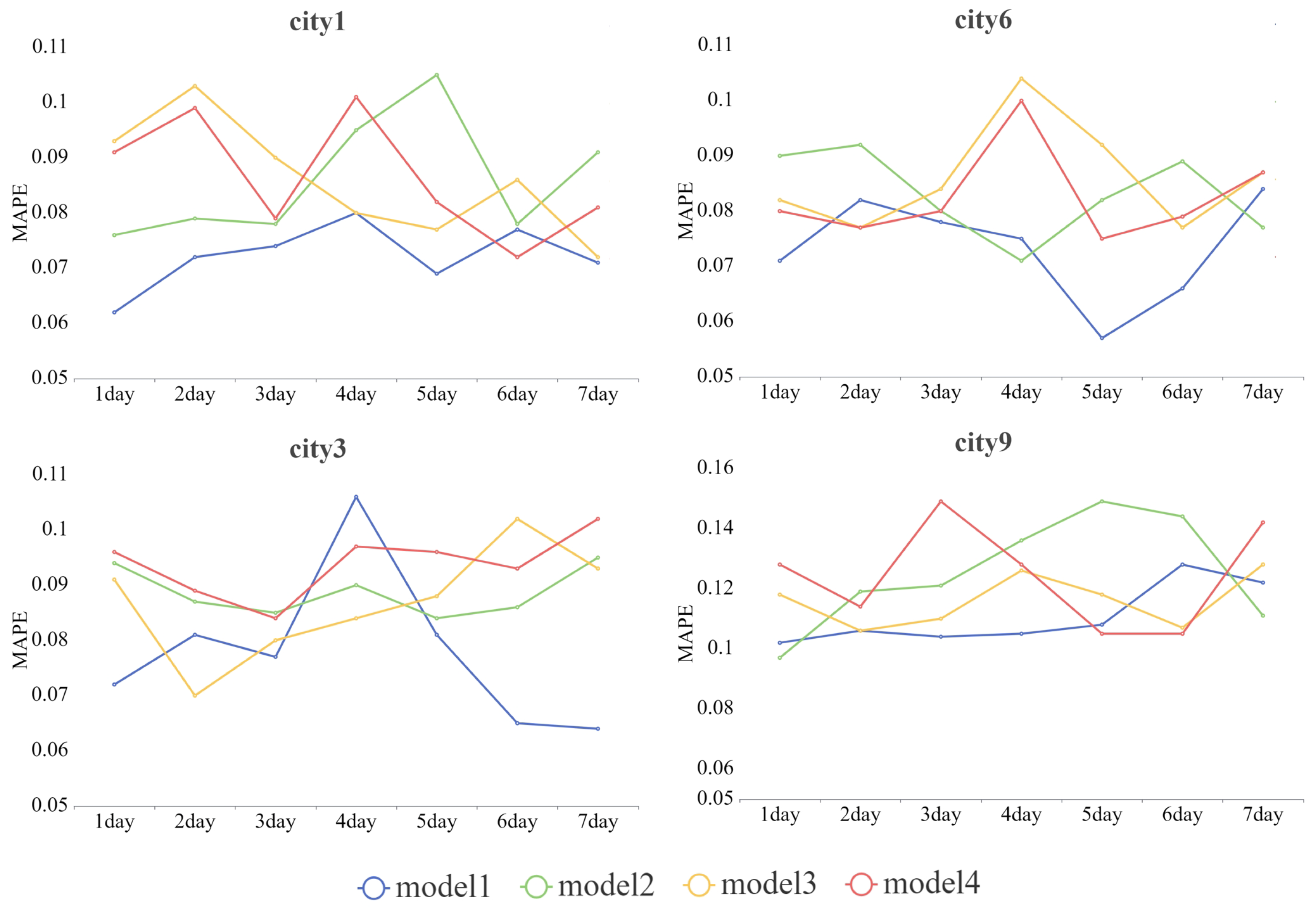
4.4. Prediction Step and Accuracy Changes

To further explore the impact of prediction step size on prediction accuracy, we conducted experiments on Model 1–4 with prediction step sizes of 1–7. The changing trend of the prediction error (MAPE) is shown in Figure 5.

As can be seen from Figure 5, in most cases, Model 1 performed well, and its prediction error was the smallest. In addition, we found that as the prediction step increased, the prediction errors of Models 2–4 showed an upward trend, while the error of Model 1 remained stable or even decreased, especially in City 3. This shows that the use of industry geographic information A and related industry $\mathcal{R}\left(j\right)$ can better capture the long-term dependency between time series, thereby improving the prediction accuracy of the model, but the duration of this long-term relationship is not fixed. For example, the prediction accuracy of City 3 improved after a step of 5 days, while the prediction accuracy of City 6 and City 9 decreased after 5 days. This may be related to the production cycle of industries in different cities, which will lead us to further study.

In City 9, the prediction accuracy was mostly greater than 0.1, which was not as good as the other three cities overall. Considering that City 9 is a mountainous city, only the straight-line distance on the plane was used, without considering detailed factors such as topography and landforms. This also makes the prediction accuracy of the model not as good as that in plain coastal cities.

For Model 2 and Model 3, their performances at different prediction steps were similar, but they were generally worse than Model 1 and better than Model 4, indicating that using geographic or related industry information can improve prediction accuracy to a certain extent. For Model 4, since it used the least amount of information, its performance was worse than Model 1 in most cases (82%), which also verifies that our Model 1 can also perform well at different prediction steps by using geographic and related industry information.

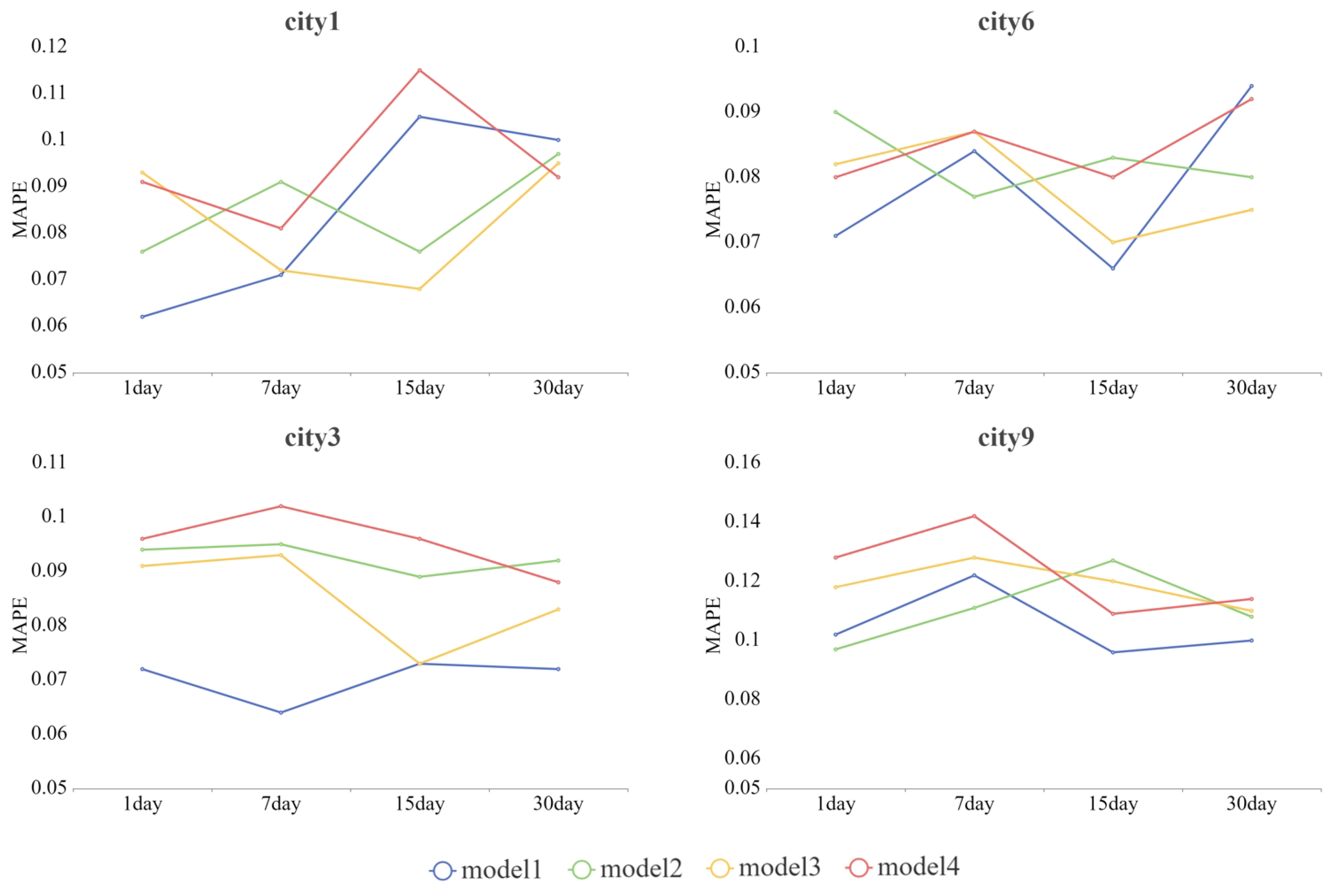
In addition, Figure 6 shows the impact of different prediction horizons on the models’ performance outcomes. We can see that, in City 3 and City 9, Model 1 demonstrated superior performance across various prediction steps, particularly at longer prediction horizons such as 15 and 30 days. In City 1 and City 6 however, the performances of different models were not stable at longer prediction horizons, even though Model 1 still performed well at short-term prediction. Therefore, the models’ performance outcomes in long-term predictions are influenced by a greater number of factors, which would not be fully captured by the graph representation model.

5. Conclusions

In this paper, we addressed the challenge of predicting industrial electricity consumption by leveraging historical electricity consumption data and geographical location information to construct an industry–geographical relationship graph. By analyzing the electricity consumption data across various industries, we built a complex network to identify relevant industries. This graph-structured data were then used as input to a graph neural network framework to capture the influence of geographical factors, same-industry relationships, related industries, and target industries. The experimental results demonstrate that our proposed IG-TFM performed well across all three key performance indicators. Comparative analysis shows that merely relying on the correlation between geographical information and data did not significantly improve the prediction accuracy. This highlights the limitations of existing methods that construct a connection matrix and employ a GCN for time series forecasting without properly selecting relevant industries. Our findings underscore the necessity and effectiveness of selecting pertinent industries based on complex networks.

Our study confirms that graph learning can effectively capture and represent the intricate relationships among industries. This enhanced representation, when used as input to the time series forcasting model, leads to a significant improvement in the accuracy of industrial electricity consumption predictions. These results validate the importance of incorporating industry–geography relationships in predictive models, thereby contributing to more accurate and reliable power consumption forecasts for industrial applications.

In this study, we simplified the geographic factors by considering only the planar distances between cities, which improved the prediction accuracy but limited the performance in mountainous regions due to the lack of topographical details. Future improvements could involve incorporating topography and using a directed graph to model industry electricity relationships, which might enhance the prediction accuracy. Additionally, the method for extracting related industries based on Formulas (5)–(8), while theoretically sound, lacks flexibility and may not perform well for specialized industries. Researching adaptive methods for learning related industries could be a valuable future direction.

References

- Klyuev, R.V.; Morgoev, I.D.; Morgoeva, A.D.; Gavrina, O.A.; Martyushev, N.V.; Efremenkov, E.A.; Mengxu, Q. Methods of forecasting electric energy consumption: A literature review. Energies 2022, 15, 8919. [Google Scholar] [CrossRef]
- Kong, X.; Li, C.; Zheng, F.; Wang, C. Improved deep belief network for short-term load forecasting considering demand-side management. IEEE Trans. Power Syst. 2019, 35, 1531–1538. [Google Scholar] [CrossRef]
- Hochreiter, S.; Schmidhuber, J. Long short-term memory. Neural Comput. 1997, 9, 1735–1780. [Google Scholar] [CrossRef] [PubMed]
- Gers, F.A.; Schmidhuber, J.; Cummins, F. Learning to forget: Continual prediction with LSTM. Neural Comput. 2000, 12, 2451–2471. [Google Scholar] [CrossRef] [PubMed]
- Salinas, D.; Flunkert, V.; Gasthaus, J.; Januschowski, T. DeepAR: Probabilistic forecasting with autoregressive recurrent networks. Int. J. Forecast. 2020, 36, 1181–1191. [Google Scholar] [CrossRef]
- Toubeau, J.F.; Bottieau, J.; Vallée, F.; De Grève, Z. Deep learning-based multivariate probabilistic forecasting for short-term scheduling in power markets. IEEE Trans. Power Syst. 2018, 34, 1203–1215. [Google Scholar] [CrossRef]
- Salinas, D.; Bohlke-Schneider, M.; Callot, L.; Medico, R.; Gasthaus, J. High-dimensional multivariate forecasting with low-rank gaussian copula processes. Adv. Neural Inf. Process. Syst. 2019, 32, 1–11. [Google Scholar]
- Qin, Y.; Song, D.; Chen, H.; Cheng, W.; Jiang, G.; Cottrell, G. A dual-stage attention-based recurrent neural network for time series prediction. arXiv 2017, arXiv:1704.02971. [Google Scholar]
- Zhou, T.; Ma, Z.; Wen, Q.; Wang, X.; Sun, L.; Jin, R. Fedformer: Frequency enhanced decomposed transformer for long-term series forecasting. In Proceedings of the International Conference on Machine Learning. PMLR, Baltimore, MD, USA, 17–23 July 2022; pp. 27268–27286. [Google Scholar]
- Xia, J.; Liu, X.; Sun, D.; Li, C.; Wang, Z. Energy Consumption Connection of Industrial Sector Based on Industrial Link Theory: A Case Study of China. Front. Ecol. Evol. 2022, 10, 897574. [Google Scholar] [CrossRef]
- Wang, X.; Si, C.; Gu, J.; Liu, G.; Liu, W.; Qiu, J.; Zhao, J. Electricity-consumption data reveals the economic impact and industry recovery during the pandemic. Sci. Rep. 2021, 11, 19960. [Google Scholar] [CrossRef]
- Luo, M.; Fan, R.; Zhang, Y. Spatial correlation of electricity consumption in China based on social network approach. IEEE Access 2020, 8, 201271–201285. [Google Scholar] [CrossRef]
- Zhou, Y.; Zhang, S.; Wu, L.; Tian, Y. Predicting sectoral electricity consumption based on complex network analysis. Appl. Energy 2019, 255, 113790. [Google Scholar] [CrossRef]
- Zhou, J.; Cui, G.; Hu, S.; Zhang, Z.; Yang, C.; Liu, Z.; Wang, L.; Li, C.; Sun, M. Graph neural networks: A review of methods and applications. AI Open 2020, 1, 57–81. [Google Scholar] [CrossRef]
- Benidis, K.; Rangapuram, S.S.; Flunkert, V.; Wang, Y.; Maddix, D.; Turkmen, C.; Gasthaus, J.; Bohlke-Schneider, M.; Salinas, D.; Stella, L.; et al. Deep learning for time series forecasting: Tutorial and literature survey. ACM Comput. Surv. 2022, 55, 1–36. [Google Scholar] [CrossRef]
- Kipf, T.N.; Welling, M. Semi-supervised classification with graph convolutional networks. arXiv 2016, arXiv:1609.02907. [Google Scholar]
- Qi, Y.; Li, Q.; Karimian, H.; Liu, D. A hybrid model for spatiotemporal forecasting of PM2.5 based on graph convolutional neural network and long short-term memory. Sci. Total. Environ. 2019, 664, 1–10. [Google Scholar] [CrossRef]
- Jiang, W.; Luo, J. Graph neural network for traffic forecasting: A survey. Expert Syst. Appl. 2022, 207, 117921. [Google Scholar] [CrossRef]
- Liu, X.; Li, W. MGC-LSTM: A deep learning model based on graph convolution of multiple graphs for PM2. 5 prediction. Int. J. Environ. Sci. Technol. 2023, 20, 10297–10312. [Google Scholar] [CrossRef]
- Diao, Z.; Wang, X.; Zhang, D.; Liu, Y.; Xie, K.; He, S. Dynamic spatial-temporal graph convolutional neural networks for traffic forecasting. In Proceedings of the AAAI Conference on Artificial Intelligence, Honolulu, HI, USA, 27 January–1 February 2019; Volume 33, pp. 890–897. [Google Scholar]
- Wang, X.; Ma, Y.; Wang, Y.; Jin, W.; Wang, X.; Tang, J.; Jia, C.; Yu, J. Traffic flow prediction via spatial temporal graph neural network. In Proceedings of the Web Conference 2020, Taipei, Taiwan, China, 20–24 April 2020; pp. 1082–1092. [Google Scholar]
- Huang, B.; Dou, H.; Luo, Y.; Li, J.; Wang, J.; Zhou, T. Adaptive spatiotemporal transformer graph network for traffic flow forecasting by iot loop detectors. IEEE Internet Things J. 2022, 10, 1642–1653. [Google Scholar] [CrossRef]
- Wu, Z.; Pan, S.; Long, G.; Jiang, J.; Chang, X.; Zhang, C. Connecting the dots: Multivariate time series forecasting with graph neural networks. In Proceedings of the 26th ACM SIGKDD International Conference on Knowledge Discovery & Data Mining, Virtual, 6–10 July 2020; pp. 753–763. [Google Scholar]
- Prim, R.C. Shortest connection networks and some generalizations. Bell Syst. Tech. J. 1957, 36, 1389–1401. [Google Scholar] [CrossRef]
- Tumminello, M.; Aste, T.; Di Matteo, T.; Mantegna, R.N. A tool for filtering information in complex systems. Proc. Natl. Acad. Sci. USA 2005, 102, 10421–10426. [Google Scholar] [CrossRef] [PubMed]
- Newman, M.E.J. Modularity and community structure in networks. Proc. Natl. Acad. Sci. USA 2006, 103, 8577–8582. [Google Scholar] [CrossRef] [PubMed]
- Dey, R.; Salem, F.M. Gate-variants of gated recurrent unit (GRU) neural networks. In Proceedings of the 2017 IEEE 60th International Midwest Symposium on Circuits and Systems (MWSCAS), Boston, MA, USA, 6–9 August 2017; IEEE: Piscataway, NJ, USA, 2017; pp. 1597–1600. [Google Scholar]