A Reduced-Order Model of a Nuclear Power Plant with Thermal Power Dispatch

Abstract

This paper presents reduced-order modeling of thermal power dispatch (TPD) from a pressurized water reactor (PWR) for providing heat to nearby heat consuming industrial processes that seek to take advantage of nuclear heat to reduce carbon emissions. The reactor model includes the neutronics of the reactor core, thermal–hydraulics of the primary coolant cycle, and a three-lump model of the steam generator (SG). The secondary coolant cycle is represented with quasi-steady state mass and energy balance equations. The secondary cycle consists of a steam extraction system, high-pressure and low-pressure turbines, moisture separator and reheater, high-pressure and low-pressure feedwater heaters, deaerator, feedwater and condensate pumps, and a condenser. The steam produced by the SG is distributed between the turbines and the extraction steam line (XSL) that delivers steam to nearby industrial processes, such as production of clean hydrogen. The reduced-order simulator is verified by comparing predictions with results from separate validated steady-state and transient full-scope PWR simulators for TPD levels between 0% and 70% of the rated reactor power. All simulators indicate that the flow rate of steam in the main steam line and turbine systems decrease with increasing TPD, which causes a reduction in PWR electric power generation. The results are analyzed to assess the impact of TPD on system efficiency and feedwater flow control. Due to the simplicity of the proposed reduced-order model, it can be scaled to represent a PWR of any size with a few parametric changes. In the future, the proposed reduced-order model will be integrated into a power system model in a digital real-time simulator (DRTS) and physical hardware-in-the-loop simulations.

1. Introduction

As of 2020, nuclear power is the most prevalent noncarbon electricity source in the United States with a 20% market share [1]. All other noncarbon energy sources combined, including hydroelectric, wind, solar, biomass, and geothermal, barely surpass nuclear power to achieve 21% market share [2]. The dramatic recent increase in intermittent wind and solar energy is changing how the power grid operates. For example, from 2000 to 2020, wind generation increased by 5945% to account for 8.4% of total generation in 2020 [2]. Over the same time period, solar power increased by 28% [3]. The proliferation of renewables is a boon for addressing the threat of climate change but also presents challenges to U.S. nuclear power. Solar and wind power have low marginal costs compared to nuclear power, and, consequently, are favored for dispatch in hourly markets. At the beginning of 2020, the United States had 98 operating nuclear power plants. By the end of 2022, this number had decreased to 94 operating reactors [4]. Potential closures for several other plants have been announced [5].

Nuclear power plants are aging and faced with competitive challenges due to relatively high operational costs compared to fossil plants. For example, gas turbines have high fuel costs but low costs when they are not operating, which enables them to curtail power without incurring excessive financial losses. In contrast, nuclear power plants have similar operational costs regardless of whether they are producing power, so curtailing power production incurs substantial financial losses. For example, the operating cost of fully depreciated nuclear is in the range of USD 31/MWh [6], which cannot compete with solar and wind in hourly markets because their operating costs are very low. Note that operating costs do not include capital costs and other costs associated with meeting firm power requirements. Including capital costs, solar power has been cited as USD 24/MWh to USD 96/MWh and the cost of onshore wind power as USD 24/MWh to USD 75/MWh [6]. The additional cost of firming the intermittency of wind and solar has been estimated to range between USD 11/MWh and USD 141/MWh.

The Light Water Reactor Sustainability (LWRS) program of the Department of Energy (DOE) is assisting utilities in nuclear power plant modernization efforts to make plants more cost-efficient as well as identifying and developing flexible plant operations and generation (FPOG) strategies that could provide diversification of revenue streams while making use of excess energy during peak hours [7].

Flexible plant operations could entail powering sustainable cryptocurrency mining and data centers, as proposed by the joint venture between Talen Energy and Terawulf, to develop a 180 MWe bitcoin mining facility [8], or it could entail providing high-quality thermal energy for industrial processes, such as high temperature steam electrolysis. Many utilities in the United States have pledged to reduce carbon emissions. For example, Arizona Public Service (APS) has pledged to become carbon neutral by 2050 and has examined the viability of producing green hydrogen from nuclear and renewables to offset carbon emissions from gas turbines during peak hours [9,10]. When considering the economics of gigawatt-hour storage, batteries are expensive to scale and lose charge over time. Hydrogen is complementary to battery storage in that it can be readily scaled and stored for long periods of time. In Utah, Advanced Clean Energy Storage (ACES) Delta, a joint venture between Mitsubishi Power Americas and Magnum Development, is developing a gigawatt-scale energy storage project utilizing underground salt caverns for compressed hydrogen storage [11].

There are different types of reactors with different operating temperatures and other characteristics. As of July 2024, there are over 400 operable reactors in the world [12,13]. Of those reactors, 307 are pressurized light water reactors (PWRs) in which the reactor coolant is pressurized, liquid water; 47 are pressurized heavy water reactors (PHWRs), and 41 are boiling light water reactors (BWRs), in which the coolant water boils in the reactor vessel [14]. This work focuses on PWRs because they are the most common. All reactors that employ water as a coolant operate at reactor temperatures of less than approximately 300 °C. Another reactor type that is increasing in importance is gas-cooled reactors, which can operate at higher temperatures, although there are less than 10 operable gas-cooled reactors in the world as of July 2024. High-temperature gas-cooled reactors are viewed as being particularly advantageous for providing high-temperature industrial heat [15,16].

Idaho National Laboratory (INL) is conducting design and engineering work to determine how to couple nuclear power plants to dispatchable industrial processes that use heat and electricity [7]. This type of coupling could enable the integrated system to flexibly provide electric power to the grid to meet peak and valley grid power demands while at the same time producing high-value nonelectric products to increase the revenue of nuclear power plants. A key objective is that participating nuclear reactors maintain steady power generation at or near 100% of the reactor power while the secondary system is maneuvered to allow for the dispatch of thermal and electrical power to coupled industrial processes. These types of flexible power dispatch operations from nuclear power plants can complement variable power from renewable energy sources, such as wind and solar power. Reduced-order modeling of these integrated system operations is crucial for investigating optimal coupling and operational strategies. However, there is a notable scarcity of reduced-order nuclear power plant model descriptions in the literature that support the modeling of coupled renewable/nuclear systems.

The nuclear power plant model in [17] offers a model for power system applications with detailed primary coolant system but uses an overly simplified secondary coolant system. In contrast, Ibrahim et al. [18] offers more detailed modeling of the secondary system but does not include the primary coolant system. Neither model considers thermal power dispatch (TPD) system. GSE’s full-scope generic PWR (GPWR) simulator can simulate plant dynamics with TPD systems, but its slower performance and limited compatibility with real-time simulation tools make it less suitable for rapid simulations.

Here, we describe the development, modeling, and results of an integrated reduced-order model that couples a pressurized water reactor (PWR) equipped with a thermal power dispatch system (RO-PWR) to an industrial process, such as high-temperature steam electrolysis. The reactor core and secondary system models are based on previously published models [17,18] and are capable of running as a dynamic simulator in real time to support hardware-in-the-loop testing and engineering evaluations. The real-time hardware-in-the-loop capabilities builds on previous work, including a Rancor Microworld model previously developed by INL and the University of Idaho [9,19]. The Rancor Microworld model incorporates a human–system interface (HMI) that emulates the control and operations of a PWR for realistic human-in-the-loop studies with representative nuclear power plant operating procedures. A separate modeling effort of this project is the implementation of a thermal power TPD system in GSE’s GPWR simulator [20].

The primary system is based on an integrated reactor with a single steam generator loop. There are currently two simulator versions, including a 160 MWt small modular reactor (SMR) with passive circulation and a 3100 MWt PWR with active circulation. The PWR model is coupled to a secondary system model with a two-stage high-pressure turbine, moisture separator reheater, three-stage low-pressure turbine, condenser, and feed water reheaters. The TPD system pulls steam from the main steam header and passes through an extraction heat exchanger and returns condensate to the condenser. The latent heat is used to vaporize water from a demineralized water source in preparation to send the demineralized steam to a high-temperature steam electrolysis (HTSE) hydrogen production facility or other industrial process. A simplified diagram of a representative system is shown in Figure 1. Heat delivery to the industrial user is modeled by a single heat exchanger. Actual thermal power dispatch operations may involve multiple heat exchangers to transfer heat to the industrial process, and the exact design of the delivery system depends upon the heat requirements of the industrial processes. Those details are outside the scope of this nuclear power plant simulation and so are not included here but can be easily captured in future work for specific applications, as needed.

The extraction of steam from the main steam header has minor impact on PWR plant operations for low levels of thermal power extraction, as described in [21]. For higher extraction levels, the most substantial impacts are in the feedwater heaters, and extracting as much as 50% of the rated reactor power may require modifying the feedwater heaters and drains to maintain guidance on mass fluxes [21].

In addition to providing steam to the coupled industrial process, the PWR may also provide electricity either behind-the-meter or through the bulk power grid, as shown in Figure 1. Implications and practicalities of providing electric power as well as heat from the PWR to industrial processes are summarized in [22].

The relative simplicity of the RO-PWR simulator provides key benefits in understanding and providing approximate validation of the results from higher-fidelity models, such as full-scope nuclear power plant simulators, which employ thousands of variables through multiple levels of coupled controls. The RO-PWR simulator was also designed to be scalable between lab-size equipment (100 kWe) and full-scale nuclear power plants (1 GWe) by adjusting only a few parameters in the models, such as fluid masses and heat exchanger areas.

This work verifies results obtained from the RO-PWR simulator by comparing those findings with results obtained from high-fidelity steady-state and transient simulations. The comparison shows that the RO-PWR simulator can reliably calculate the steady-state and transient response of a PWR plant for thermal power dispatch and is beneficial in explaining nuanced relationships between key parameters, including those between steam flows in the TPD system, turbine system, FWHs, and the main steam lines. With these verifications, the RO-PWR simulator can provide a basis to assess the performance of future simulations that include dispatching electric or thermal power in integrated energy systems.

2. Modeling and Integration

Figure 2 shows the schematic diagram of the overall system and is similar to Figure 1, except that additional details are included to increase the accuracy of the representation. The PWR consists of two separate coolant loops: a primary coolant circuit to carry heat produced in the core, and a secondary coolant circuit to utilize the heat for electricity and heat applications. The steam generator utilizes heat from the primary coolant circuit to produce steam in the secondary loop. The secondary coolant circuit distributes a part of the generated steam to the extraction steam line (XSL) that provides heat for the industrial process and sends the remainder of the steam to the turbines to produce electricity [19]. The feedwater heater train includes two high-pressure feedwater heaters that receive extraction steam from the high-pressure turbine, and three low-pressure feedwater heaters that receive extraction steam from the low-pressure turbines. Although actual Westinghouse PWRs feature three low-pressure similar turbines, the RO-TPD simulator combines those entities into a single, equivalent turbine. Similar to Figure 1, steam is extracted from the main steam line, passed through a condensing heat exchanger, and then the condensate is sent to the condenser. Heat from the condensing heat exchanger is used to boil demineralized water to create steam for the coupled industrial process. High-voltage electricity from the switchyard is also dispatched to the industrial process.

The following subsections explain the equations used in the proposed RO-PWR simulator.

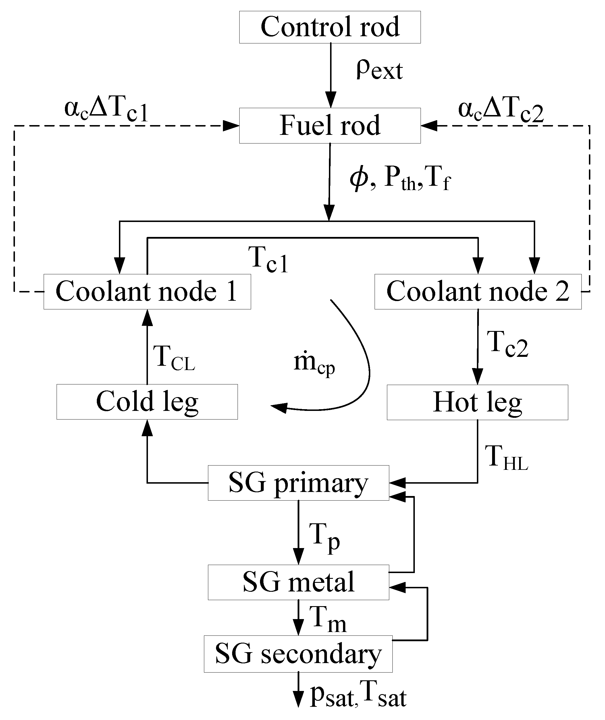
2.1. Primary Coolant System

The primary coolant system follows the approach described by Poudel, Joshi, and Gokaraju [17]. Figure 3 shows the schematic diagram of the reactor primary coolant system with the reactor core interfacing with the secondary system through a steam generator. The reactor core model captures the neutron dynamics within the core, as well as the thermal hydraulics and convection heat transfer in the primary coolant system. The reactor core model assumes that the pressure in the reactor pressure vessel (RPV) is constant to simplify the simulation (perfect pressurizer control). This assumption is valid inasmuch as the primary system is not subjected to any dramatic transients during simulations, which is consistent with the key objective of the modeling to maintain the primary system at nearly steady state while flexing the secondary system.

Core neutronics is approximated as the average neutron flux from a lumped kinetics model that includes a single energy model and a neutron precursor group that includes six groups of delayed neutrons:

$$\begin{array}{c}{\displaystyle \frac{d\varphi }{dt}}={\displaystyle \frac{\rho -\beta }{\Lambda }}\varphi +\lambda C\\ {\displaystyle \frac{dC}{dt}}={\displaystyle \frac{\beta }{\Lambda }}\varphi -\lambda C\end{array}$$

(1)

where $\varphi$ is the average neutron flux which is proportional to the reactor thermal power $P_{th}$, C is the delayed neutron precursor concentration, $\beta$ is the delayed neutron fraction with a value of 0.007, $\Lambda$ is prompt neutron lifetime with a value of 2 × 10⁻⁵ s, and $\lambda$ is the decay constant with a value of 0.1.

The net core reactivity ($\rho$) is determined as the total contribution of reactivity from fuel and moderator temperature feedback and control rod operation and is expressed as follows:

$$\rho ={\rho }_{ext}+{\alpha }_f\Delta T_f+0.5{\alpha }_c\left(\Delta T_{c1}+\Delta T_{c2}\right)$$

(2)

The heat transfer between the fuel lumps and primary coolant is estimated using Mann’s model [23]. Within the core region, primary coolant is represented by two nodes. The behavior of fuel and primary coolant temperatures are given by

$$\begin{array}{c}{\displaystyle \frac{d{T}_f}{dt}}={\displaystyle \frac{\tau P_{th}^r\varphi +h_{fc}{A}_{fc}\left(T_{c1}-T_f\right)}{m_f{c}_{pf}}}\\ {\displaystyle \frac{d{T}_{c1}}{dt}}={\displaystyle \frac{(1-\tau )P_{th}^r\varphi +h_{fc}{A}_{fc}\left(T_f-T_{c1}\right)}{m_c{c}_{pc}}}+{\displaystyle \frac{2{\dot{m}}_{cp}\left(T_{CL}-T_{c1}\right)}{m_c}}\\ {\displaystyle \frac{d{T}_{c2}}{dt}}={\displaystyle \frac{(1-\tau )P_{th}^r\varphi +h_{fc}{A}_{fc}\left(T_f-T_{c1}\right)}{m_c{c}_{pc}}}+{\displaystyle \frac{2{\dot{m}}_{cp}\left(T_{c1}-T_{c2}\right)}{m_c}}\end{array}$$

(3)

The model can represent primary coolant flow as either passive or active circulation. In active circulation, primary coolant flow is regulated using a recirculation pump. In passive circulation, the temperature difference between the hot leg and cold leg creates a natural buoyancy force to vertically carry the coolant through the reactor core.

$${\dot{m}}_{NC}={\dot{m}}_{NC}^r\sqrt[3]{P_{th}/P_{th}^r}$$

(4)

$${\dot{m}}_{cp}=\left\{\begin{array}{cc}\hfill {\dot{m}}_{\mathrm{pump}},& \mathrm{active}\mathrm{circulation}\hfill \\ \hfill {\dot{m}}_{NC},& \mathrm{passive}\mathrm{circulation}\hfill \end{array}\right.$$

(5)

The mean temperatures of the hot and cold leg regions are approximated using first-order linear functions:

$$\begin{array}{c}{\displaystyle \frac{d{T}_{HL}}{dt}}={\displaystyle \frac{T_{c2}-T_{HL}}{{\tau }_{HL}}}\\ {\displaystyle \frac{d{T}_{CL}}{dt}}={\displaystyle \frac{2T_p-T_{HL}-T_{CL}}{{\tau }_{CL}}}\end{array}$$

(6)

where ${\tau }_{HL}=m_{HL}/{\dot{m}}_{cp}$ and ${\tau }_{CL}=m_{CL}/{\dot{m}}_{cp}$ are the residence times of the respective coolant lumps representing the lags in heat transport. Note that the above equations constitute an approximate reactor model that is sufficient for capturing the transient impact of the reactor on the secondary side of the nuclear plant. It does not include the more detailed reactor modeling that is needed for fuel burn-up studies, such as in [24,25,26].

2.2. Steam Generator

The steam generator (SG) is represented using the simplified three-lump model advocated by Ali [27]. In this approach, the primary coolant, tube metal, and secondary coolant are modeled as separate lumped masses with temperatures $T_p$, $T_m$, and $T_{sat}$. Heat transfer between the lumped masses is based on their average temperature. The secondary coolant enters the steam generator in liquid state with pressure psat and exits as saturated vapor at the same pressure $p_{sat}$. The thermodynamics of the steam generator is governed by (7).

$$\begin{array}{c}{\displaystyle \frac{d{T}_p}{dt}}=K_{HL}\left(T_{HL}-T_p\right)+{\displaystyle \frac{K_m\left(T_m-T_p\right)}{2}}\\ {\displaystyle \frac{d{T}_m}{dt}}=K_{mp}\left(T_p-T_m\right)+K_{ms}\left(T_{sat}-T_m\right)\\ {\displaystyle \frac{d{p}_{sat}}{dt}}={\displaystyle \frac{\left(K_{sm}\left(T_m-T_{sat}\right)-{\dot{m}}_{cs}\left(U_v-c_{pi}{T}_{fi}\right)\right)}{K_s}}\end{array}$$

(7)

where $K_{HL}={\dot{m}}_{cp}{m}_p^{-1}$, $K_m=h_{pm}{A}_{pm}{m}_p^{-1}{c}_p^{-1}$, $K_{mp}=h_{pm}{A}_{pm}{m}_m^{-1}{c}_m^{-1}$, $K_{ms}=h_{ms}{A}_{ms}{m}_m^{-1}{c}_m^{-1}$, $K_{sm}=h_{ms}{A}_{ms}$, $K_s=m_{sw}{\displaystyle \frac{d{U}_w}{dp}}+m_{sv}{\displaystyle \frac{d{U}_v}{dp}}-m_{sv}{U}_{wv}{v_{wv}}^{-1}{\displaystyle \frac{d{v}_g}{dp}}$, $U_{wv}=U_v-U_w$, and $v_{ww}=v_v-v_w$.

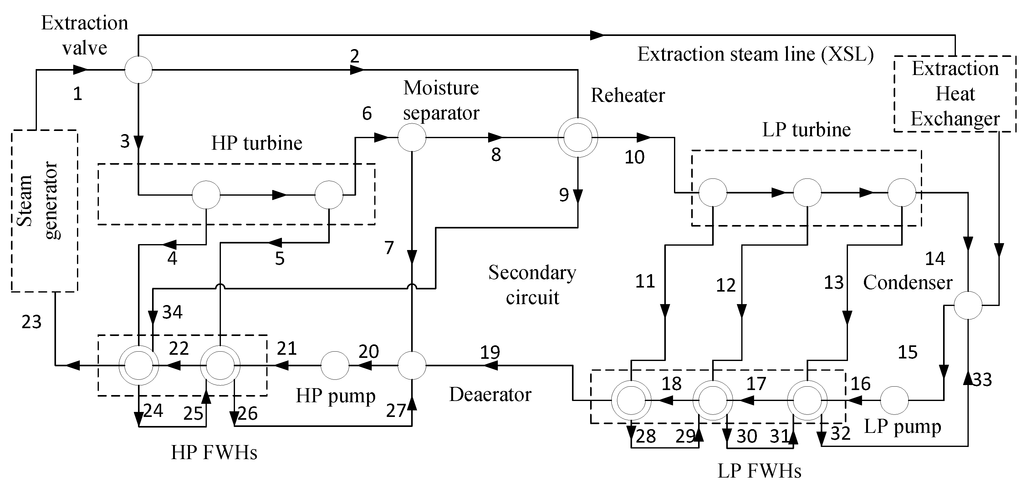
2.3. Secondary Coolant System

The model of the secondary coolant circuit follows that developed by Ibrahim et al. [18]. The secondary side includes two high-pressure (HP) turbine stages, three low-pressure (LP) turbine stages, a moisture separator and reheater (MS/R), a deaerator, two HP feedwater heaters (HP-FWHs), three LP feedwater heaters (LP-FWHs), a condenser, one LP pump, and one HP pump. The steam dump line from the main steam line to the condenser, as featured in typical PWRs, is also included in the model. However, an extraction heat exchanger is included in the turbine bypass (steam dump) line, labeled as XSL. The extraction heat exchanger uses heat from the main steam line to generate demineralized steam for the industrial heat-consuming process. Figure 4 shows a nodal illustration of the integrated system. Each circle corresponds to a component/element in the secondary circuit that alters the thermodynamic state of the coolant. The concentric circles represent closed-loop heat exchangers with the main flow in the inner circle (tube side) and the heating liquid in the outer circle (shell side). The node numbers at the output of different components represent the thermodynamic stages considered in the secondary coolant circuit model. The thermodynamic state is represented by pressure ($p_i$), temperature ($T_i$), enthalpy ($h_i$), entropy ($s_i$), and vapor quality ($x_i$) in addition to mass flow rate ${\dot{m}}_i$, where the subscript “i” refers to the node numbers in Figure 4.

2.3.1. Thermodynamic State Calculation

The secondary side is represented by quasi-static mass and energy balance equations. The quasi-static representation is sufficient due to the relatively slow transitions in these simulations. The following design assumptions are made for the pressure and mass flow rates at different nodes in the secondary coolant loop:

• At steady state, steam exiting the steam generator is saturated. The same assumption was made earlier with the steam generator model, i.e., $T_1=T_{sat}$ and $p_1=p_{sat}$. Considering a standard operating condition, steam pressure $p_{sat}$ is known for a given reactor power level.

  $$p_1=p_{sat}=f_{Pp}\left(P_{th}\right)$$

  (8)

  where $f_{Pp}$ provides the saturated steam pressure at a given reactor thermal power.
• Changing the TPD extraction level will result in fluctuation of steam pressure at the SG outlet. To maintain the main steam at the given pressure setpoint, the feedwater control system regulates the feedwater supply to the steam generator. Therefore, the feedwater flow rate is an unknown variable that should be calculated at the given TPD extraction level.
• Pressure drop of steam across the valves is negligible. The pressure drops across the moisture separator, reheater, FWHs, feedwater lines, and deaerator are negligible.
• The heat addition in the SG, reheater, and FWHs and the heat rejection in the condenser are adiabatic processes. The pressure values at the inlets and outlets of these equipment are equal.
• Assuming the valve positions for turbine extraction and reheater lines are changed together for different TPD extraction levels, the relative flow resistances of the turbine and feedwater lines also remain the same. Thus, the ratios of flows through different lines and the ratios of pressure drops do not change. The pressure of the steam extracted from a turbine is proportional to the turbine inlet pressure.
• The LP and HP pumps are controlled to maintain their pressure output in a constant ratio with $p_1$.

Based on these assumptions, the pressure at different nodes of the secondary coolant circuit can be considered a ratio of steam pressure at the outlet of steam generator:

$$p_i=a_i\ast p_1\forall i\in \{XSL,2-34\}$$

(9)

where $a_i$ is the pressure ratio for the ith node, which remains constant for given design of secondary coolant loop. Also, based on the above assumptions, pressure ratios in the main steam and feedwater lines are related as follows:

$$\begin{array}{cc}& a_2=a_3=a_{XSL}=1,\hfill \\ & a_6=a_7=a_8=a_{10}=a_{16}=a_{17}=a_{18}=a_{19}=a_{20}=a_{27},\hfill \\ & a_{14}=a_{33}=a_{15},a_{21}=a_{22}=a_{23}=1.\hfill \end{array}$$

And the pressure ratios at extraction phases and FWH lines are related as follows:

$$\begin{array}{cc}& a_9=a_2,a_{34}=a_{24}=a_4,a_{25}=a_{26}=a_5\hfill \\ & a_{28}=a_{11},a_{29}=a_{30}=a_{12},a_{31}=a_{32}=a_{13}.\hfill \end{array}$$

Note that the feedwater supply to the steam generator is also dependent on the TPD extraction level. The steam flow to the XSL is controlled based on a flow setpoint as a ratio of main steam flow. Based on the above assumptions, the mass flow rates at different nodes of the secondary circuit can be presented as fixed ratios of the main steam flow:

$${\dot{m}}_j=b_j\ast {\dot{m}}_1\forall j\in \{XSL,2-34\},$$

(10)

where $b_j$ is the flow ratio for jth node, which remains constant for a given operating condition. Also, based on the above assumptions, the flow ratios in main steam and feedwater lines are related as follows:

$$\begin{array}{cc}& b_7=b_6\left(1-x_6\right),b_8=b_{10}=b_6{x}_6,b_2=b_9=b_{34},\hfill \\ & b_{15}=b_{16}=b_{17}=b_{18}=b_{19}=b_{XSL}+b_{14}+b_{33},b_{33}=b_{11}+b_{12}+b_{13},\hfill \\ & b_{20}=(1-x_{20}^{\prime })\ast \left(b_7+b_{19}+b_4+b_5+b_2\right),b_{23}=b_{22}=b_{21}=b_{20},\hfill \end{array}$$

where $x_6$ is the steam fraction of the mixture at the inlet of moisture separator and $x_{20}^{\prime }$ is the steam fraction of the two-phase mixture inside the deaerator. Similarly, the flow ratios at extraction phases and FWH lines are related as follows:

$$\begin{array}{cc}& b_{24}=b_{25}=b_4+b_{34},b_{26}=b_{27}=b_5+b_{25},\hfill \\ & b_{28}=b_{29}=b_{11},b_{30}=b_{31}=b_{29}+b_{12},\hfill \\ & b_{32}=b_{33}=b_{31}+b_{13}.\hfill \end{array}$$

It is evident from the above relationships that the flow rates in the secondary circuit can be expressed as ratios of ${\dot{m}}_1$ as long as $x_6$ and $x_{20}^{\prime }$ are known for a given operating condition. However, ${\dot{m}}_1$ is an unknown variable for a given TPD extraction level. Once the pressure values at different nodes and flow ratios are identified for the secondary coolant circuit, the remaining thermodynamic state variables and the mass flow rate at a given thermal power level can be calculated using the water and steam properties from Steam Tables [28]. Detailed equations for the secondary side thermodynamic state calculation are provided in Appendix A.

2.3.2. Absolute Mass Flow

Equations (A1)–(A32) show the calculation of thermodynamic states of different nodes in the secondary coolant circuit for a given reactor power level without the knowledge of mass flow rates. Now, with the thermodynamic state of the feedwater at the SG inlet known, the steam flow required to maintain the SG outlet at the rated operating condition is calculated as follows:

$${\dot{m}}_1={\dot{m}}_{23}={\displaystyle \frac{P_{th}}{h_1-h_{23}}}$$

(11)

The mass flow rates at all other stages of the secondary coolant circuit can be calculated using Equation (10).

2.3.3. Turbine Power Output

The mechanical power output of HP and LP turbines is given as follows:

$$P_m={\eta }_T{W}_{net}={\eta }_T\left(W_{HPT}+W_{LPT}-W_{HPP}-W_{LPP}\right)$$

(12)

where ${\eta }_T$ is the turbine efficiency and $W_{net}$ is the useful work for electricity. The calculation of $W_{HPT}$, $W_{LPT}$, $W_{HPP}$, and $W_{LPP}$ is shown in Appendix A.

2.3.4. Thermal Power Dispatch

As shown in Figure 2, XSL receives steam from the secondary coolant circuit and provides heat to the demineralized water in the delivery steam line (DSL). The extraction heat exchanger absorbs the latent heat from the steam supplied to the XSL and uses that heat to boil water in the DSL. The isobaric heat extraction from the XSL means that:

$$\begin{array}{cc}\hfill & p_{XSL}^{\mathrm{out}}=p_{XSL}\mathrm{and}{x}_{XSL}^{\mathrm{out}}=0\hfill \\ \hfill & h_{XSL}^{\mathrm{out}},T_{XSL}^{\mathrm{out}},s_{XSL}^{\mathrm{out}}=f_{px}\left(p_{XSL}^{\mathrm{out}},x_{XSL}^{\mathrm{out}}\right)\hfill \end{array}$$

(13)

where the superscript “out” refers to the fluid at the outlet of the extraction heat exchanger on the condenser side. The heat supplied to the DSL ($Q_{DSL}$) is given as follows:

$$Q_{DSL}={\dot{m}}_{XSL}\ast \left(h_{XSL}-h_{XSL}^{\mathrm{out}}\right)$$

(14)

Based on Equation (14), the percentage of TPD is defined as

$$\%TPD={\displaystyle \frac{{\dot{m}}_{XSL}}{{\dot{m}}_1}}\ast \left({\displaystyle \frac{h_{XSL}-h_{XSL}^{\mathrm{out}}}{h_1-h_{23}}}\right)$$

(15)

2.4. Coupled Industrial Process

Results are presented in this paper for dispatching 15%, 30%, and 50% of the reactor thermal power to a coupled industrial process, such as clean hydrogen production. High-temperature steam electrolysis (HTSE) is a dispatchable industrial process that could enable dispatching nuclear power to the bulk power grid according to grid demand. HTSE is an efficient hydrogen production method because it uses steam as a feedstock instead of condensed water and because the electric power required to split water is reduced at high temperatures. At the appropriate scales, HTSE is projected to become competitive with SMR hydrogen production, capable of providing carbon-free hydrogen to the market [22,29]. The optimum ratio of thermal power input to electric power input for HTSE is approximately 1 to 4 [22]. There are other industrial processes, such as producing synthetic fuels or high-value chemicals from carbon dioxide and other low-value feedstocks, that require higher ratios of thermal power input to electric power. Extracting higher levels of thermal power to support those processes is also explored in this work, although it is recognized that extracting more than approximately 50% of the rated reactor power may not be feasible due to equipment and licensing safety limitations [21]. In that regard, this work complements other published works that have explored coupling light water reactors to hybrid thermochemical processes based on magnesium and chloride compounds and copper and chlorine compounds [30,31] by providing additional details on how the TPD could impact nuclear power plant operations and by enabling coupled dynamic simulations.

2.5. Model Initialization

An initialization sequence is developed for the model to initiate the system at any steady-state condition, enabling it to be integrated with a power system model. This same block can be used for quasi-static simulation of the system for nondynamic assessments. At the start of the simulation, the values of the reactor power level and the percentage of steam extracted to the XSL are treated as input parameters. The main steam pressure is treated as being dependent on the reactor power level and the percentage of steam extracted to the XSL. The remaining variables are determined from calculations starting from those three variables. The initialization algorithm proceeds as illustrated in Figure 5.

Once the system is initialized with steady conditions, dynamic simulations can be started. During simulations in which the RO-PWR simulator is transitioned from one state to another, such as 0% steam extraction to 15% steam extraction, the extraction flow controller steps the setpoint for percent steam extraction (%TPD) to follow a linear ramp. A proportional integral (PI) controller adjusts the feedwater flow rate to the steam generator (${\dot{m}}_{23}$) as needed to keep the temperature and pressure of the main steam ($T_1$ and $p_1$, respectively) constant for the given reactor power level. This control is necessary because the temperature of the feedwater entering the steam generator ($T_{23}$) depends upon the percent steam extraction (%XSL). This dependency arises because the heat provided to the FWHs comes from the turbine system and decreases as the percentage of steam extraction increases. Although it is intended that the reactor power remains constant during the simulation, another PI controller is integrated to operate control rods to maintain the average primary coolant temperature constant at a reference setpoint. The LP and HP feedwater pumps are also controlled to maintain their outlet pressure in a fixed ratio with main steam pressure.

2.6. Model Integration and Simulation

The previous version of Rancor microworld [9] was implemented in the C# programming language for Microsoft’s .NET Framework, so that it could be easily used as part of a Windows Presentation Foundation (WPF) application. This version of the model uses the Rancor microworld framework implemented in the Python programming language. It is broadly compatible with Python versions 3.6, 3.7, and 3.8 across Windows 10 (Anaconda, python.org), macOS (homebrew), and GNU/Linux (Ubuntu packages). The model requires NumPy 1.26.2, Matplotlib 3.8.3 (for generating plots), and iapws 1.5.3. The Rancor microworld framework provides functionality normally found in a plant simulator, such as the ability to create initial conditions, load initial conditions, run the model in real time with two-way communication, and data logging. The architecture follows an object-oriented programming paradigm with a class for an SMR model and a class for a PWR with a secondary system that inherits the SMR class. A steady-state hydrogen plant model class can be used independently or coupled to the PWR/secondary/TDS. The hydrogen plant model will determine generated flow, electrical load, and cooling load based on saturated steam flow and temperature from the TDS. A data historian is implemented as a third class that supports the integrated models.

3. Results

The reactor was validated by comparing the system parameters to the published model by Poudel, Joshi, and Gokaraju [17] and by conducting a series of pseudo-transient tests while having the automated rod control system maintain $p_{sat}$ and observing the response of the system parameters. Once the Python implementation of the model was verified to behave as expected, parameters were identified to scale the model up to a gigawatt-scale reactor based on GPWR models [18,20] and Fortran plant code (see

Table 1. RO-SMR vs. RO-PWR simulator parameters.

Parameter	RO-SMR	RO-PWR
	(160 MWt)	(2900 MWt)
Mass of fuel lump (kg)	11,252	82,000
Heat transfer area of fuel to coolant (m2)	583	4415
Primary coolant volume (m3)	1.879	160
Circulation (kg/s)	Passive up to 586.86	Active at 14,267
Volume of cold loop (m3)	26.8	50.76
Volume of hot loop (m3)	9.7	14
Volume of primary coolant in the SG (m3)	3.564	30.5
Heat transfer area of primary to SG metal lump (m2)	1123	25,272 †
Heat transfer area of SG metal lump to secondary (m2)	1214	42,615 †
Secondary steam pressure (MPa)	2.71	6.89
Volume of SG (m3)	13.391	70.08

† Parameterized to match hot and cold loop RCS temperatures.

). The heat transfer parameters were adjusted to achieve RCS cold and hot loop temperatures typical of PWRs.

Table 2. Full-scope GPWR vs. RO-PWR simulator parameters.

Parameter	GPWR (2900 MWt)	RO-PWR (2900 MWt)
Secondary pressure (MPa)	6.89	6.89
Primary coolant flow (kg/s)	14,267	14,267
Cold loop temperature (°C)	292.3	285.88
Hot loop temperature (°C)	326.8	322.29

compares the system parameters of the RO-PWR simulator with those of the full-scope GPWR simulator.

3.1. Secondary System Validation

As previously described, the secondary system was modeled after Ibrahim et al. [18] and the node numbering in Figure 4 is consistent with that of Figure 2 of Ibrahim et al. [18] allowing for direct comparisons between node states. While the secondary side configuration is identical to Ibrahim et al., we noticed that the pressure at the main steam header was not at the rated condition. Therefore, the main steam pressure has been adjusted to match the conditions of Ibrahim et al. for secondary system validation.

Table 3. Thermodynamic data for the secondary system with %TPD = 0.

Node	Name	T	p	h	s	x	$\dot{\mathit{m}}$
		°C	MPa	kJ/kg	kJ/kg·°C		kg/s
1	gv	289	7.38	2767	5.79	1.00	1652
2	ms_reheater	289	7.38	2767	5.79	1.00	176
3	hpt	289	7.38	2767	5.79	1.00	1476
4	hpt_stg1	253	4.17	2685	5.83	0.93	157
5	hpt_stg2	216	2.16	2594	5.89	0.89	103
6	hpt_stg3	180	0.99	2492	5.96	0.86	1216
7	deaerator	180	0.99	761	2.14	0.00	172
8	reheater	180	0.99	2777	6.59	1.00	1044
9	reheater_hpfwh1	289	7.38	1287	3.16	0.00	176
10	lpt	288	0.99	3026	7.08	1.00	1044
11	lpt_stg1	201	0.39	2864	7.19	1.00	72
12	lpt_stg2	113	0.13	2700	7.32	1.00	66
13	lpt_stg3	70	0.03	2526	7.47	0.96	54
14	lpt_stg4	33	0.01	2336	7.65	0.91	851
15	cond_mix	33	0.01	139	0.48	0.00	1044
16	cpump	33	0.99	140	0.48	0.00	1044
17	lpfwh3	66	0.99	277	0.90	0.00	1044
18	lpfwh2	103	0.99	431	1.34	0.00	1044
19	lpfwh1	139	0.99	587	1.73	0.00	1044
20	fwpump_suction	164	0.99	695	1.99	0.00	1652
21	fwpump	165	7.38	702	1.99	0.00	1652
22	hpfwh2	197	7.38	841	2.29	0.00	1652
23	hpfwh1	234	7.38	1012	2.64	0.00	1652
24	hpfwh1_stm_out	253	4.17	1099	2.82	0.00	333
25	hpfwh2_stm2	216	2.16	1099	2.84	0.09	333
26	hpfwh2_stm_out	216	2.16	926	2.48	0.00	436
27	deaerator_hpfwh_stm	180	0.99	926	2.50	0.08	436
28	lpfwh1_stm_out	143	0.39	602	1.77	0.00	72
29	lpfwh2_stm2	106	0.13	602	1.79	0.07	72
30	lpfwh2_stm_out	106	0.13	446	1.38	0.00	138
31	lpfwh3_stm2	70	0.03	446	1.40	0.07	138
32	lpfwh3_stm_out	70	0.03	292	0.95	0.00	193
33	cond_fw	33	0.01	292	0.98	0.06	193
34	hpfwh1_stm2	253	4.17	1287	3.18	0.11	176

presents the thermodynamic data for the RO-PWR secondary model with no TPD. The temperature–entropy (T–S) and pressure–enthalpy (P–h) diagrams of the turbines are included in Appendix B and Figure A5 and show the variations of those parameters in the turbine system.

The results from the RO-PWR simulator are mostly within 5% of the Ibrahim et al. model with only a few exceptions. Discrepancies between the models that are greater than 5% are presented in

Table 4. Thermodynamic discrepancies with Ibrahim et al.’s model [18]. Discrepancies outside the ±5% bounds are highlighted.

Node	T	p	h	s	x	$\dot{\mathit{m}}$
6	0.0%	0.0%	0.5%	0.5%	0.8%	−10.3%
12	6.3%	0.0%	0.4%	0.4%	0.0%	3.5%
20	−8.5%	0.0%	−8.8%	−7.0%	0.0%	39.5%
21	−8.8%	0.0%	−9.0%	−7.3%	0.0%	2.7%
22	−7.2%	0.0%	−7.5%	−5.9%	0.0%	2.7%
23	−5.8%	0.0%	−6.3%	−4.8%	0.0%	2.7%
24	0.0%	0.0%	0.0%	0.0%	0.0%	117.5%
25	0.0%	0.0%	0.0%	0.0%	0.2%	117.5%
26	0.0%	0.0%	0.0%	0.0%	0.0%	72.0%
27	0.0%	0.0%	0.0%	0.0%	0.1%	226.3%

. The largest discrepancies (greater than 10%) are all mass flow rates. In the model by Ibrahim et al., mass flow is not properly conserved at some nodes, which is the cause of the discrepancies. For example, in the model by Ibrahim et al., the mass flows entering the high-pressure turbine from the SG and exiting towards the HP FWHs and MSR are not balanced. The first HP FWH receives steam from the first stage of the HP turbine and the reheater. The mass flow exiting the first HP FWH at node 24 should be the sum of these two flows (nodes 4 and 9). In this instance, the Ibrahim et al. model fails to conserve mass, and the RO-PWR simulator corrects this error. The discrepancy for node 20 is also explained by the Ibrahim et al. model failing to conserve mass, in this instance, from the suction of the HP feedwater pump to the outlet. Assuming that the level in the deaerator remains constant, the mass flow for node 20 should be the sum of nodes 7, 19, and 27. There is a different reason for the temperature discrepancy at node 12. The RO-PWR simulator has lower isentropic efficiency for turbine expansion compared to that of Ibrahim et al. [18], so that steam remains superheated after the first stage of LPT expansion at node 12 for the RO-PWR simulator. In the model by Ibrahim et al., the steam at this location is saturated.

In the RO-PWR simulator, the feedwater temperatures/enthalpies through nodes 20–23 are lower than in the Ibrahim et al. model because that model assumes that the deaerator outlet pressure and enthalpy (and therefore temperature) are condensed from the moisture separator (node 7). However, the deaerator also receives flow from the shell side of the LP FWHs and tube side of the HP FWHs. In the RO-PWR simulator, the enthalpy of the HP feedwater pump inlet (node 20) is determined by energy balance from all three deaerator inlets before determining temperature and entropy. In summary, the discrepancies between the two models are explained, and the RO-PWR simulator appears to reasonably model the steady-state response of a PWR secondary system.

3.2. Thermal Power Dispatch System Validation

A key feature of the RO-PWR simulator design is that steam delivered to the industrial process is isolated from the steam extracted from the main steam line by heat exchangers to reduce the risk of contaminants escaping from the nuclear protected zone. For the purposes of process control, the temperature of the steam sent to the industrial process in the DSL (Figure 2) is assumed to be constant at 251.6 °C, such that the flow rate of water entering the XSL heat exchanger is adjusted to the level of TPD. Figure 6 provides the energy balance of the XSL heat exchangers for 15% TPD. For convenient representation, the heat exchange is represented as occurring in two parts with a demineralized (demin) water preheater and a reboiler. To achieve 15% TPD, 169.7 kg/s of steam is extracted from the main steam line, and 160.7 kg/s of saturated steam is sent to the industrial process through the DSL.

3.3. Integrated Model Results

The predicted steam flows in the main steam line and XSL are shown in Figure 7 for 0%, 15%, 30%, and 50% TPD. For each simulation, the percentage of TPD was gradually increased over a time period of approximately 32 min, held constant for approximately the same time period and then ramped down. The TPD process follows the same approach described by Hancock et al. [20]. That work employed a validated, full-scope, high-fidelity simulator from GSE Systems to model various levels of TPD. Limitations of that work are that it did not specify detailed plant impacts due to TPD operations, and the results of the simulations were not fully described and validated to ensure accuracy.

For the simulations in this work, the primary side control (reactivity control) was disabled, so the control rods could not move as the flow in the XSL increased. Increasing XSL flow results in a decrease in turbine flow, which in turn results in a proportional decrease in extraction flows towards the HP and LP FWHs. With less heat available at the FWHs, the temperature of the preheated feedwater entering the steam generator at node 23 decreases. To maintain the main steam supply temperature at node 1 at the rated setpoint, the secondary side controller reduces the feedwater flow rate, causing the main steam flow rate to decrease. The result is that as the percentage of TPD increases, the temperature of the feedwater entering the SG and the mass flow rate in the main steam line both decrease. With the secondary side modeled as a quasi-static system, the fluctuations seen on the primary side are very small, even though the primary system is modeled with detailed dynamics.

Figure 8 shows predicted steady-state values of mass flow in the main steam line and the turbine systems for different levels of TPD ranging from 0% to 100% and includes applicable results reported by Ibrahim et al. [18], Hancock et al. [20], and also by Sargent and Lundy (S&L) for a 4-loop PWR (labeled as “S&L, 4-loop” [21]. For their work, S&L used a validated steady-state commercial software called PEPSE (Performance Evaluation of Power System Efficiencies) to determine impacts on a 4-loop PWR due to 0%, 30%, 50%, and 70% TPD. The PEPSE model neglects heat losses and makes other linear assumptions that likely affect the accuracy of the simulation at high values of TPD. The most striking feature of Figure 8 is that the results from all of the TPD models collapse onto nearly identical lines. The results from Ibrahim et al. [18] are outliers compared to the other models because the turbines in that model are assumed to be isentropic, as explained above.

An important point is that, as per Equation (15), the percentage of TPD is higher than the percentage of mass flow dispatched from the main steam line to the XSL. With the assumption in this work that the condensate from the industrial process returns at a temperature of 49 °C and enthalpy of 211.1 kJ/kg, the percentage of main steam flow that is dispatched to the XSL for different levels of TPD can be calculated using Equation (15). We find that for TPD levels of 30%, 50%, and 70%, the corresponding percentages of main steam flow that is dispatched to the XSL are 22.6%, 37.6%, and 52.7%. As noted above, the work of Hancock et al. [20] is based on a validated, full-scope, high-fidelity simulator of a 3-loop PWR from GSE Systems to model various levels of TPD [20]. In that work, the percentage of TPD is defined as the percentage of main steam flow that is dispatched to the XSL, such that the percentage of TPD heat includes the heat from the reactor as well as the heat in the feedwater. In Figure 8, the TPD values from Hancock et al. [20] are adjusted to make their levels consistent with Equation (15).

As noted above, an important aspect of TPD is that the temperature of the feedwater entering the steam generator decreases with increasing levels of TPD because steam flow from the turbine system to the feedwater heaters decreases with increasing TPD. Figure 9 shows the decrease in the temperature of the feedwater entering the SG as predicted by the different models. The results from the RO-PWR simulator and the full-scope GSE Systems simulator (Hancock et al. [20]) predict that TPD has substantially more impact on the feedwater temperature than predicted by the PEPSE model developed by S&L. The differences between the results obtained from the RO-PWR simulator and the PEPSE model developed by S&L are not surprising because the PEPSE model is much more complex and more closely resembles the secondary system of a real 4-loop Westinghouse PWR. Combining the feedwater extraction lines and the moisture separator/reheater lines in the RO-PWR simulator, as shown in Figure 4, is expected to result in a predicted loss of heat recuperation in the feedwater heaters, such that it is expected that the RO-PWR simulator will overpredict the impact of TPD on feedwater temperature compared to a real plant. S&L’s PEPSE model has been thoroughly validated, and the modifications made to the model for TPD are well within the model capabilities for up to 50% TPD. Mass and energy balances of the PEPSE model have been carefully checked, so those results are expected to closely match anticipated potential TPD operations in real PWRs. The fact that results from the full-scope, high-fidelity 3-loop Westinghouse PWR simulator modified for TPD operations by Hancock et al. [20] match those of the RO-PWR simulator rather than the predictions of the detailed PEPSE model are likely due to simplifications in the Hancock model. Differences between the models for 3-loop and 4-loop PWRs may also be partially responsible for the discrepancies between the Hancock and PEPSE model results in Figure 9.

Figure 10 shows the steady-state values of mass flow in the main steam line and the turbine systems for increasing levels of TPD, as calculated by the different models presented in this work. The flow of steam in the main steam line decreases with increasing TPD because colder feedwater requires more thermal energy to heat to the saturated pressure specification of the main steam line. The heat available from the reactor is limited, so the flow of steam secondary fluid through the steam generator and the main steam line must decrease with increasing TPD. The results from S&L and Hancock et al. for the effect of increasing TPD on main steam flow are in excellent agreement, while the RO-PWR simulator indicates a greater decrease in main steam flow with increasing TPD. Regarding steam flow in the HP turbine, the results from the S&L PEPSE model indicate that as TPD increases, the ratio of main steam moving to the HP turbine increases relative to that of steam moving to the moisture separator reheater (MSR). This effect is manifest in the slopes of lines fitted to the HP turbine steam flow in Figure 10. The coefficients from a least-squares regression fit to the S&L PEPSE model for the steam flow in the HP turbine are shown and indicate that the reduction in the steam flow to the HP turbine is only 87% of the increase in steam flow for TPD, which is only possible if less main steam flows to the MSR. Figure 10 also shows the combined turbine shaft work predicted as a function of TPD. According to the S&L PEPSE model, the impact of TPD on the combined turbine shaft work is nearly identical to the TPD level, such that a TPD of 50% of the reactor power causes the turbine shaft work to decrease by approximately 50%. Interestingly, the results from the RO-PWR simulator and Hancock et al. [20] simulator indicate that the steam flow in the HP turbine and the combined turbine shaft power are all similar to the percent of TPD, indicating that these models may not fully account for losses in the turbines at lower steam flow rates and lower pressures.

4. Conclusions

This paper describes the modeling and validation of a generic reduced-order thermal power dispatch pressurized water reactor (RO-PWR) simulator to support the analysis of PWR operations during electrical and thermal power dispatch. The detailed modeling equations and model integration were followed by steady-state and dynamic validation using existing simulators and models. The results indicate that the simulator can reliably calculate the steady-state and transient response of a PWR plant for thermal power dispatch. The RO-PWR simulator proved beneficial in explaining nuanced key relationships between parameters, including those between steam flows in the TPD system, turbine system, FWHs, and the main steam lines.

The RO-PWR simulator is intended to be coupled to reduced-order models of industrial processes and grid simulators to study thermohydraulic feedback and grid interactions. It can run in real time and communicate through a web API, which allows it to be integrated with physical systems for potential hardware-in-the-loop testing. There are opportunities for improving the RO-PWR simulator. For example, the simplified models of the moisture separate/reheater (MSR) and feedwater heaters sacrifice heat that could be recovered from the turbines and cause the temperature of feedwater to excessively drop with increasing thermal power dispatch (TPD). This simplification accelerates the calculation speed of the simulator to support real-time operator-in-the-loop studies and is expected to have minimal impact on the fidelity of grid-level simulations that probe the interactions between nuclear power plants and other energy resources, such as solar and wind power, during transient simulations.

The current configuration of the RO-PWR simulator extracts steam directly from the main steam line such that the saturated steam in the XSL line may be hotter than is needed by some industrial processes. Extracting TPD steam after the HP turbine could potentially yield greater efficiency for the integrated energy system by reducing the amount of wasted heat in the XSL line feeding an HTSE plant. This more efficient design has been suggested in the literature [22]. Future RO-PWR models could examine alternative steam extraction configurations.

References

1. Francis, M. Renewables Became the Second-Most Prevalent U.S. Electricity Source in 2020. Available online: https://www.eia.gov/todayinenergy/detail.php?id=48896 (accessed on 14 July 2024).
2. U.S. Energy Information Administration (EIA). Electrical Generation from Wind; U.S. Energy Information Administration (EIA): Washington, DC, USA, 2021.
3. Tyra, B.; Cassar, C.; Harrison, E.; Wong, P.; Yildiz, O. Electrical Power Monthly. February 2021. Available online: https://www.eia.gov/electricity/monthly (accessed on 14 July 2024).
4. U.S. Nuclear Regulatory Commission (NRC). List of Power Reactor Units. Available online: https://www.nrc.gov/reactors/operating/list-power-reactor-units.html (accessed on 14 July 2024).
5. Scott, M.; Comstock, O. Despite Closures, U.S. Nuclear Electricity Generation in 2018 Surpassed Its Previous Peak. 2019. Available online: https://www.eia.gov/todayinenergy/detail.php?id=38792 (accessed on 14 July 2024).
6. Bilicic, G.; Scroggins, S. 2023 Levelized Cost of Energy+; Lazard: Hamilton, Bermuda, 2023. [Google Scholar]
7. Light Water Reactor Sustainability Program. Reports. Available online: https://lwrs.inl.gov/SitePages/Reports.aspx (accessed on 14 July 2024).
8. World Nuclear News. US Companies Announce Plans for Nuclear-Powered Bitcoin Mine. 2021. Available online: https://www.world-nuclear-news.org/Articles/US-companies-announce-plans-for-nuclear-powered-bi (accessed on 14 July 2024).
9. Ulrich, T.; Boring, R.; Lew, R. Extrapolating Nuclear Process Control Microworld Simulation Performance Data from Novices to Experts—A Preliminary Analysis. In Advances in Human Error, Reliability, Resilience, and Performance; Boring, R.L., Ed.; Springer: Cham, Switzerland, 2019; pp. 283–291. [Google Scholar]
10. John, J.S. Arizona Public Service Lays out Its Options for Reaching Zero-Carbon Energy by 2050. Green Tech Media. 30 June 2020. Available online: https://www.greentechmedia.com/articles/read/arizona-utility-aps-charts-path-to-zero-carbon-energy-by-2050 (accessed on 14 July 2024).
11. Advanced Clean Energy Storage (ACES) Delta. Delivering Hydrogen, Driving Clean Energy for the Western U.S. Available online: https://aces-delta.com/about-us/ (accessed on 14 July 2024).
12. World Nuclear Association. Reactor Database. Available online: https://world-nuclear.org/nuclear-reactor-database (accessed on 14 July 2024).
13. Statista Research Department. Operable Nuclear Power Reactors Worldwide 2024, by Country; Statista Research Department: Hamburg, Germany, 2024. [Google Scholar]
14. Statista Research Department. Number of Operable Nuclear Reactors Worldwide as of July 2024, by Reactor Type; Statista Research Department: Hamburg, Germany, 2024. [Google Scholar]
15. Nuclear Energy Agency. High-Temperature Gas-Cooled Reactors and Industrial Heat Applications; Technical Report NEA No. 7629; Organisation for Economic Co-Operation and Development: Paris, France, 2022. [Google Scholar]
16. González Rodríguez, D.; Brayner de Oliveira Lira, C.A.; García Hernández, C.R.; Roberto de Andrade Lima, F. Hydrogen production methods efficiency coupled to an advanced high-temperature accelerator driven system. Int. J. Hydrogen Energy 2019, 44, 1392–1408. [Google Scholar] [CrossRef]
17. Poudel, B.; Joshi, K.; Gokaraju, R. A Dynamic Model of Small Modular Reactor Based Nuclear Plant for Power System Studies. IEEE Trans. Energy Convers. 2020, 35, 977–985. [Google Scholar] [CrossRef]
18. Ibrahim, S.M.A.; Ibrahim, M.M.A.; Attia, S.I. The Impact of Climate Changes on the Thermal Performance of a Proposed Pressurized Water Reactor: Nuclear-Power Plant. Int. J. Nucl. Energy 2014, 2014, 793908. [Google Scholar] [CrossRef]
19. Westover, T.; Hancock, S.; Shigrekar, A. Monitoring and Control Systems Technical Guidance for LWR Thermal Energy Delivery; Technical Report NL/EXT-20-57577; Idaho National Laboratory: Idaho Falls, ID, USA, 2020.
20. Hancock, S.; Westover, T.; Luo, Y. Evaluation of Different Levels of Electric and Thermal Power Dispatch Using a Full-Scope PWR Simulator; Technical Report INL/EXT-21-63226; Idaho National Laboratory: Idaho Falls, ID, USA, 2020.
21. Westover, T.; Brown, J.; Fidlow, H.; Gaudin, H.; Miller, J.; Miller, K.; Neimark, G.; Richards, N.; Kut, P.; Paugh, C.; et al. Light Water Reactor Sustainability (LWRS) Program Report: Preconceptual Designs of 50% and 70% Thermal Power Extraction Systems; Technical Report INL/RPT-24-77206, Rev. 0; Idaho National Laboratory: Idaho Falls, ID, USA, 2024.
22. Westover, T.; Boardman, R.; Abughofah, H.; Amen, G.; Fidlow, H.; Garza, I.; Klemp, C.; Kut, P.; Rennels, C.; Ross, M.; et al. Light Water Reactor Sustainability Program Report: Preconceptual Designs of Coupled Power Delivery between a 4-Loop PWR and 100–500 MWe HTSE Plants; Technical Report INL/RPT-23-71939; Idaho National Laboratory: Idaho Falls, ID, USA, 2023.
23. Kerlin, T.W.; Katz, E.M.; Thakkar, J.G.; Strange, J.E. Theoretical and Experimental Dynamic Analysis of the H. B. Robinson Nuclear Plant. Nucl. Technol. 1976, 30, 299–316. [Google Scholar] [CrossRef]
24. Castagna, C.; Aufiero, M.; Lorenzi, S.; Lomonaco, G.; Cammi, A. Development of a Reduced Order Model for Fuel Burnup Analysis. Energies 2020, 13, 890. [Google Scholar] [CrossRef]
25. Chersola, D.; Lomonaco, G.; Marotta, R. The VHTR and GFR and their use in innovative symbiotic fuel cycles. Prog. Nucl. Energy 2015, 83, 443–459. [Google Scholar] [CrossRef]
26. Kępisty, G.; Oettingen, M.; Stanisz, P.; Cetnar, J. Statistical error propagation in HTR burnup model. Ann. Nucl. Energy 2017, 105, 355–360. [Google Scholar] [CrossRef]
27. Ali, M.R.A. Lumped Parameter, State Variable Dynamic Models for Utube Recirculation Type Nuclear Steam Generators. Ph.D. Thesis, University of Tennessee, Knoxville, TN, USA, 1976. Available online: https://trace.tennessee.edu/utk_graddiss/2548/ (accessed on 14 July 2024).
28. Haar, L.; Gallagher, J.; Kell, G. NBS/NRC Steam Tables: Thermodynamic and Transport Properties and Computer Programs for Vapor and Liquid States of Water in SI Units; Hemisphere Publishing Corporation: New York, NY, USA, 1984; p. 320. [Google Scholar]
29. Prosser, J.H.; James, B.D.; Murphy, B.M.; Wendt, D.S.; Casteel, M.J.; Westover, T.L.; Knighton, L.T. Cost analysis of hydrogen production by high-temperature solid oxide electrolysis. Int. J. Hydrogen Energy 2024, 49, 207–227. [Google Scholar] [CrossRef]
30. Ozcan, H.; Dincer, I. Thermodynamic modeling of a nuclear energy based integrated system for hydrogen production and liquefaction. Comput. Chem. Eng. 2016, 90, 234–246. [Google Scholar] [CrossRef]
31. Al-Zareer, M.; Dincer, I.; Rosen, M.A. Development and assessment of a novel integrated nuclear plant for electricity and hydrogen production. Energy Convers. Manag. 2017, 134, 221–234. [Google Scholar] [CrossRef]
Figure 1. Simplified diagram of the RO-PWR simulator with coupling to a high-temperature electrolysis (HTSE) hydrogen (H2) production plant.
Energies 17 04298 g001
Figure 2. Diagram of the RO-PWR simulator with multiple feedwater heater stages and the primary coolant system.
Energies 17 04298 g002
Figure 3. Schematic diagram of reactor primary system interfacing with steam generator and secondary coolant system.
Energies 17 04298 g003
Figure 4. Nodal representation of PWR secondary coolant circuit.
Energies 17 04298 g004
Figure 5. Initialization sequence of the RO-PWR simulator.
Energies 17 04298 g005
Figure 6. Thermodynamic balance of TPD from model with 15% TPD extraction.
Energies 17 04298 g006
Figure 7. Predicted flows in the main steam line and XSL for 0%, 15%, 30%, and 50% TPD.
Energies 17 04298 g007
Figure 8. Destination of reactor heat for increasing levels of TPD as calculated by different models, including the RO-PWR model presented in this work.
Energies 17 04298 g008
Figure 9. Decrease in feedwater temperature entering the steam generator (stream 23 in Figure 4) for increasing levels of TPD as determined by different models.
Energies 17 04298 g009
Figure 10. Steam flow in the main steam line (stream #1 in Figure 4) and turbine system (stream #3 in Figure 4) as well as combined turbine shaft work as functions of TPD as determined by different models.
Energies 17 04298 g010