Research on Hybrid Logic Dynamic Model and Voltage Predictive Control of Photovoltaic Storage System

Abstract

This paper investigates microgrid systems characterized by the coexistence of discrete events and continuous events, a typical hybrid system. By selecting the charging and discharging processes of the energy storage unit as logical variables, a mixed logical dynamic (MLD) model for the microgrid in islanded mode is established. Based on this model, model predictive control (MPC) theory is employed to optimize the energy management strategy, aiming to stabilize the DC bus voltage of the photovoltaic (PV) unit and minimize the switching frequency of the energy storage unit’s charging and discharging processes during system operation.

1. Introduction

Due to factors such as energy shortages, environmental pressures, inherent flaws in large-scale power systems, and global electricity market reforms, distributed generation technology has become a research hotspot for the development of national power systems worldwide. Distributed generation refers to modular power generation technology that utilizes dispersed energy sources near the load, offering advantages such as localized power supply, low line losses, high comprehensive energy utilization, and good environmental compatibility [1,2]. Compared to traditional centralized power generation and distribution methods, distributed generation has several advantages: high reliability of power supply, reduced environmental pollution, and autonomous control for users. However, the uncontrollability and randomness of distributed power sources also pose certain disadvantages, such as high single-unit access costs and adverse effects on the current power system under high penetration rates. Therefore, to better integrate the advantages of distributed generation technology and mitigate its adverse impacts on the main grid, researchers have proposed an intelligent organization form of distributed generation systems-microgrids [3].

A microgrid refers to a small-scale power generation and distribution system composed of distributed generation sources, energy storage devices, energy conversion devices, local loads, and monitoring and protection devices. It can achieve self-control, protection, and management. Microgrids can operate in two modes: connected to the main grid or in an independent island mode [4,5]. By optimally combining various types of distributed generation equipment with different inherent characteristics, microgrids can enhance the reliability and quality of power supply on the user side. Energy storage devices, as a crucial component of microgrid systems, provide strong support for improving the capacity to integrate renewable energy and for quickly and accurately tracking load changes. Monitoring and protection devices enhance the power control capability of microgrids, providing necessary technical support for the optimal use of renewable energy, mitigating energy distribution imbalances, and delivering high-quality electrical power [6,7,8].

Therefore, vigorously developing microgrid technology and integrating it with the current power systems to form a flexible new power supply pattern can effectively enhance the reliability and security of China’s power system. It provides an effective approach to improving the current power system’s supply capacity and power quality. Additionally, it offers theoretical support for optimizing the current power system structure and constructing a robust and fully controllable smart grid. Simultaneously, promoting microgrid technology in China is a concrete manifestation of pursuing sustainable development. It holds significant importance for adjusting the energy structure, addressing electricity needs in rural and remote areas, protecting the environment, implementing a scientific development concept, and building a harmonious society.

Due to its flexible and intelligent control capabilities and extensive use of distributed generation technology, the microgrid has become a vital component in the development of national power industries and the formulation of energy strategies worldwide. Currently, some countries and regions are accelerating the research and testing of microgrids, proposing development plans that align with local energy policies and the current state of their power systems.

Table 1. The Microgrid demonstration projects.

Microgrid Demonstration Projects	Country	Description
CERTS test bed	United States	The system utilizes three 60 kW micro gas turbines, with three feeders including two capable of islanding operation. This setup facilitates testing the dynamic characteristics of various components of the microgrid [9,10].
Boston Bar IPP	Canada	The system comprises two 3.45 MW hydroelectric generators supplying power to users through a 120/25 kV substation. It is capable of conducting islanding operation tests [11].
Kythnos Islands Microgrid	Greece	The system utilizes a 400 V distribution network to supply electricity to 12 households on Kisnos Island. It includes six photovoltaic units totaling 11 kW, one 5 kW diesel generator, and one 3.3 kW battery energy storage unit. Its primary purpose is to test the system’s peak load capacity and reliability [12].
Hachinohe project	Japan	The system is equipped with three units of 170 kW gas turbines and a 50 kW photovoltaic unit. Its primary objective is to mitigate energy supply-demand imbalance issues during system operation [13].
Hefei University of Technology Microgrid Demonstration Project	China	Established in collaboration with the University of New Brunswick, Canada, the system includes wind and photovoltaic units with a total capacity of 200 kW. It is capable of islanding operation to supply power to a campus building [14].

presents some of the microgrid demonstration projects from both domestic and international initiatives.

In recent years, the application of hybrid systems and related theories in the analysis of power electronic systems has emerged as a new research focus. References [15,16] have utilized hybrid system theory to establish hybrid logical dynamic models and switching models for different types of power electronic converters, optimizing control methods accordingly. References [17,18] have investigated circuit fault diagnosis and parameter identification based on the actual operating modes of power electronic converters. However, current research on hybrid theory for power electronic systems primarily focuses on DC/DC or DC/AC converters, with limited comprehensive studies addressing broader issues in power electronic systems.

Due to the fact that the switching actions of various devices and the charging/discharging processes of energy storage units in microgrids can be viewed as discrete events, while the operational states of individual units in these discrete states can be seen as continuous events, microgrids can be fundamentally viewed as hybrid systems. Therefore, leveraging concepts and theories from hybrid systems can analyze the operational characteristics of microgrids effectively. In a microgrid, the control actions of the power electronic devices such as inverters at the interfaces of various units, as well as the charging/discharging actions of energy storage units, can be considered as “0,1” binary discrete events. Meanwhile, the state variables of the system in different discrete states continuously evolve over time, constituting a continuous process. Hence, microgrid systems can be fundamentally seen as hybrid systems.

Currently, the application of hybrid theory in the field of power electronics mainly focuses on modeling, parameter identification, and fault diagnosis of power electronic converters. However, comprehensive studies addressing broader issues in power electronic systems are still lacking [15,16,17,18].

This paper addresses the typical hybrid nature of microgrid systems, which involve both discrete and continuous events. It selects the charging/discharging processes of energy storage units as logical variables and establishes a mixed logical dynamic (MLD) model for microgrid operation in islanded mode. Based on this model, the paper applies model predictive control (MPC) theory to optimize energy management strategies, aiming to simultaneously stabilize the DC bus voltage of photovoltaic units and reduce the switching frequency of energy storage unit charging/discharging during system operation.

2. Hybrid Model of Microgrid Systems

A hybrid system refers to a system where discrete and continuous events interact internally. Discrete events typically manifest as scheduling instructions, switch toggling, and sensor activations, while continuous events involve the continuous evolution of system states over time under specific conditions. Therefore, leveraging relevant theories to establish hybrid models and optimize operational characteristics is meaningful, especially in addressing the hybrid nature observed in microgrid systems. Figure 1 depicts the structural composition of the small-scale microgrid system designed in this paper. It includes two photovoltaic units with equalized control, one battery energy storage unit, a central controller, and local loads, all connected to the AC bus. Additionally, the central controller communicates with lower-level controllers via a bus to achieve overall system management and scheduling.

2.1. Hybrid System Model

According to the treatment of hybrid systems, they can be classified into two main categories based on the coupling degree of their discrete and continuous events: “aggregation” and “extension” [19]. The former corresponds to the overall system displaying characteristics of a discrete event dynamic system, distinguishing different continuous state spaces and focusing on the system’s discrete characteristics. The latter treats the system according to the characteristics of a continuous variable dynamic system exhibited by the entire system in the form of a set of differential equations, with discrete events in the system enabling or disabling specific states within the equation set.

2.1.1. “Aggregation” Class Models

A typical “aggregation” class model is the hierarchical structure model, which describes its internal continuous events using differential equations. The states of discrete events, time-driven system transitions, and state transition functions are described in the form of automata. The transformation between discrete events and continuous events is achieved through event generators and actuators. Currently, commonly used tools for describing such models include Finite State Automata and Petri Nets.

• Finite State Machine

Finite State Automata models were initially applied in computer science to analyze discrete event systems. They describe state space transitions using a finite number of vertices representing the state space and arcs between them. This method has later been shown to have promising applications in hybrid systems as well.

A finite state automaton can be described using a five-tuple $\mathrm{A}$

$$\mathrm{A}= (Q,\sum ,\delta ,q_0,F)$$

(1)

where $Q$ is the finite set of states; $\sum$ is the finite symbol set (or alphabet); $\delta :Q\times \sum \to Q$ is the state transition function; $q_0\in Q$ is the initial state; $F\subseteq Q$ is the set of accepting states.

2.

Petri Grid

Petri nets focus on the organizational structure and dynamic behavior of systems. They primarily address state transitions that a system can undergo, transition conditions, relationships between different states, and the impact of state transitions on the system. However, Petri nets do not concern themselves with the physical characteristics of the system itself.

A Petri net can be represented by a quadruple $N$:

$$N=(P,T,I,O)$$

(2)

where $P=\{p_1,p_2\cdots ,p_{\mathrm{m}}\}$, $m\ge 0$ and $T=\{t_1,t_2\cdots ,t_n\}$, $n\ge 0$ denote finite sets of places and transitions in the system respectively. There is no intersection between $P$ and $T$. $I=\{I(t_1),I(t_2),\cdots ,I(t_{\mathrm{m}})\}$ represents the input function from transitions to places, and $O=\{O(t_1),O(t_2),\cdots ,O(t_{\mathrm{m}})\}$ represents the output function from places to transitions.

Petri nets, as a strict superset of automata models, exhibit higher language complexity and are more compact in their descriptions of possible states by using markings. This compactness ensures that the structure of the net remains within a smaller range even as the system’s state space increases. Despite their more complex marking rules, Petri nets facilitate better modeling of system concurrency and conflicts through synchronized handling of system phenomena. Moreover, this tool also offers advantages such as graphical representation and distributed characteristics in terms of system states.

2.1.2. “Extension” Class Models

“Extension” class modeling methods are primarily applied to switching systems with logical transformation characteristics. These methods are designed based on the characteristics of different state spaces to optimize the sequence of switching control, enabling controllers to switch between different state spaces. The main objective is to ensure the stability of the switching process.

• Mixed Logical Dynamic (MLD) Model

Considering the characteristics and implementation requirements of industrial production processes, Swedish process control expert Morari proposed a novel system modeling framework—Mixed Logic Dynamic Model—based on hybrid system theory. This model integrates discrete and continuous variables, incorporating logic judgment rules, expert systems, and discrete input sets.

A typical MLD model can be represented as:

$$\left\{\begin{array}{l}x(t+1)=Ax(t)+B_{1}u(t)+B_2\delta (t)+B_{3}z(t)\\ y(t)=Cx(t)+D_{1}u(t)+D_2\delta (t)+D_{3}z(t)\\ E_2\delta (t)+E_{3}z(t)\le E_{1}u(t)+E_{4}x(t)+E_5\end{array}\right.$$

(3)

where $t\in Z$, $x(t)={[x_{\mathrm{c}}(t),x_{\mathrm{l}}(t)]}^{\mathrm{T}}$ is the system state, with $x_{\mathrm{c}}(t)\in R^{\mathrm{nc}}$ representing the continuous state of the system and $x_{\mathrm{l}}(t)\in {\{0,1\}}^{\mathrm{nl}}$ representing the discrete state of the system; $y(t)={[y_{\mathrm{c}}(t),y_{\mathrm{l}}(t)]}^{\mathrm{T}}$ is the system output vector, with $y_{\mathrm{c}}(t)\in R^{\mathrm{nc}}$ representing the continuous output and $y_{\mathrm{l}}(t)\in {\{0,1\}}^{\mathrm{nl}}$ representing the discrete output; $u(t)={[u_{\mathrm{c}}(t),u_{\mathrm{l}}(t)]}^{\mathrm{T}}$ is the system control input variable, with $u_{\mathrm{c}}(t)\in R^{\mathrm{nc}}$ representing the continuous input and $u_{\mathrm{l}}(t)\in {\{0,1\}}^{\mathrm{nl}}$ representing the discrete input; ${\delta }_{\mathrm{l}}(t)\in {\{0,1\}}^{\mathrm{nl}}$ represents auxiliary logic variables; and $z_{\mathrm{c}}(t)\in R^{\mathrm{nc}}$ represents auxiliary continuous variables.

The MLD model incorporates the logical relationships between state spaces, switching conditions, and control input constraints within a unified modeling framework. It explicitly describes the relationships among system inputs, states, and outputs, thereby extending the linear system model to hybrid systems. In practice, the MLD model integrates expert experience and qualitative knowledge of the system under different states during the modeling process. It synthesizes the interdependencies between various physical quantities, constraints, and state switching logic rules. Logical judgments and operations within the system are converted into Boolean logic propositions, which are ultimately transformed into corresponding integer linear inequality constraints that include both discrete and continuous variables.

2.

Switching System Models

Switching systems can be regarded as a collection of system differential equations and their switching control rules. The controller manages the system’s transitions between different state spaces. The primary goal is to ensure the stability of the controller during the switching process.

Typical switching systems can be represented as:

$$H=(D,F)$$

(4)

where $D=(I,E)$ denotes a finite state machine, $I=\{1,2,\cdots ,m\}$, $E=I\times I$ represents a set of discrete events, and $F=\{f_{\mathrm{i}}:R^{\mathrm{n}}\times R^{\mathrm{m}}\to R^{\mathrm{n}},i\in I\}$ constitutes a collection of subsystem vector fields.

The hybrid nature described by switching system models involves the system transitioning between different continuous state spaces according to specified logical switching rules. Within each state space, the system operates according to specific dynamic characteristics. The switching rules in such models can be based on time, space, or logic.

In cases where there exist locally unstable sub-state spaces within the system, stability of the entire hybrid system can be ensured by constructing appropriate switching strategies. Similarly, even if each subsystem maintains local stability within its respective space, ensuring overall system stability necessitates imposing corresponding constraints on the switching processes between these subspaces.

2.2. Modeling of Hybrid Systems Using MLD Models

Currently, many controlled systems incorporate components with binary logic characteristics, such as relay contacts opening or closing, transistor switches conducting or non-conducting, or valve opening and closing actions. The evolution of these actions can be understood as following if-then-else rules. Such systems are typically controlled based on practical conditions and operational experience, often using rule-based control tables rather than differential equations or discrete equations for description.

However, MLD models, as an extension of linear dynamic systems in hybrid systems, not only encompass the continuous dynamic events of the system but also include its discrete states, the interactions between the two, and the relevant constraints on control inputs. Therefore, accurately depicting the characteristics of the system is of significant importance.

2.2.1. The Mathematical Foundation of MLD Modeling

• Propositional Logic and its Fundamental Conversion Relations

Propositional logic, also known as Boolean logic, is the simplest formal system of logic, where the fundamental element is a statement with a definite truth value [20]. A proposition is typically denoted by $X$, where $X=\mathrm{T}$ indicates the proposition is true, and $X=\mathrm{F}$ indicates it is false. Through basic operators and equivalence relations in Boolean algebra, individual propositions can be combined to express more complex propositions. Moreover, complex propositions can be transformed into simpler combinations of propositions.

Table 2. Conversion rules of propositional logic.

Name	Conversion Relations
Law of Equivalence	$P\leftrightarrow Q=(P\to Q)\wedge (Q\to P)$
Implication Law	$P\to Q=(\neg P\vee Q)$
Associative Law	$\begin{array}{l}P\wedge (Q\vee R)=(P\wedge Q)\vee (P\wedge R)\\ P\vee (Q\wedge R)=(P\vee Q)\wedge (P\vee R)\end{array}$
De Morgan’s Law	$\begin{array}{l}\neg (P\vee Q)=(\neg P\wedge \neg Q)\\ \neg (P\wedge Q)=(\neg P\vee \neg Q)\end{array}$

illustrates the fundamental conversion relations in propositional logic.

2.

Propositional Logic and Linear Integer Inequalities

In hybrid systems, discrete events can be described using linear integer inequalities that include logical variables and binary variables.

Define binary variables ${\delta }_i\in \{0,1\}$, $i\in N^{+}$ such that they correspond to the truth value of propositions $X_i$; if $X_i=\mathrm{T}$, then ${\delta }_i=1$; if $X_i=\mathrm{F}$, then ${\delta }_i=0$. Hence, there exist the following equivalent relations of mixed integer inequalities containing propositional logic and binary variables.

$$X_1\vee X_2\iff {\delta }_1+{\delta }_2\ge 1$$

(5)

$$\neg X_1\iff {\delta }_1=0$$

(6)

$$X_1\wedge X_2\iff {\delta }_1=1, {\delta }_2=1$$

(7)

$$X_1\leftrightarrow X_2\iff {\delta }_1-{\delta }_2=0$$

(8)

$$X_1\to X_2\iff {\delta }_1-{\delta }_2\le 0$$

(9)

$$X_1\oplus X_2\iff {\delta }_1+{\delta }_2=1$$

(10)

3.

Propositional Logic and Mixed Linear Integer Inequalities

If a logical proposition involves both logical variables and continuous variables, it can be termed as a mixed continuous logical proposition. Such propositions primarily describe the coupling between discrete events and continuous variables in hybrid systems, necessitating their description through constraints formulated as mixed linear integer inequalities.

Define $f(x):R^{\mathrm{n}}\to R$, $f(x)\in [m_{\mathrm{x}},M_{\mathrm{x}}]$ where $f(x)\le 0$ is the corresponding binary variable. The relationship between $f(x)$ and $\delta$ is as follows:

$$[f(x)\le 0]\wedge [\delta =1]\iff f(x)-\delta \le -1+m_{\mathrm{x}}(1-\delta )$$

(11)

$$[f(x)\le 0]\vee [\delta =1]\iff f(x)\le M_{\mathrm{x}}\delta$$

(12)

$$\neg [f(x)\le 0]\iff f(x)\ge \epsilon$$

(13)

$$[\delta =1]\to [f(x)\le 0]\iff f(x)\ge M_{\mathrm{x}}(1-\delta )$$

(14)

$$[f(x)\le 0]\to [\delta =1]\iff f(x)\ge \epsilon +(m_{\mathrm{x}}-\epsilon )\delta$$

(15)

$$[f(x)\le 0]\leftrightarrow [\delta =1]\iff \left\{\begin{array}{l}f(x)\le M_{\mathrm{x}}(1-\delta )\\ f(x)\ge \epsilon +(m_{\mathrm{x}}-\epsilon )\delta \end{array}\right.$$

(16)

Here, $\epsilon$ is the tolerance factor (relaxation factor), typically chosen based on the controller’s computational precision.

For the binary product ${\delta }_1{\delta }_2$, it can be linearized and transformed into the following inequality relationship by introducing auxiliary variable ${\delta }_3={\delta }_1{\delta }_2$:

$${\delta }_3={\delta }_1{\delta }_2\iff \left\{\begin{array}{l}-{\delta }_1+{\delta }_3\le 0\\ -{\delta }_2+{\delta }_3\le 0\\ {\delta }_1+{\delta }_2-{\delta }_3\le 1\end{array}\right.$$

(17)

For the product of a binary variable and a continuous variable $\delta f(x)$, introduce an auxiliary variable $z=\delta f(x)$ such that:

$$\left\{\begin{array}{l}[\delta =0]\to [z=0]\\ [\delta =1]\to [z=f(x)]\end{array}\right.$$

(18)

Based on the fundamental conversion relations of logical propositions and Formulas (15) and (16), we can derive:

$$z=\delta f(x)\iff \left\{\begin{array}{l}z\le M_{\mathrm{x}}\delta \\ z\ge f(x)-M_{\mathrm{x}}(1-\delta )\\ z\ge m_{\mathrm{x}}\delta \\ z\le f(x)-m_{\mathrm{x}}(1-\delta )\end{array}\right.$$

(19)

2.2.2. Steps for MLD Model Construction

The MLD model transforms system logical judgments, heuristic rules, and inherent constraints into propositional logic form. It then utilizes the logic propositions to derive mixed linear integer inequalities incorporating discrete and continuous variables to obtain system-related constraints. The main steps are as follows:

(1)

Establish the state space model of the continuous part of the system based on actual operating conditions, while setting auxiliary logical variables for different operational modes or regions.

(2)

Address nonlinear components, logical expressions, control inputs, and their inherent constraints within the system using conversion rules to establish corresponding mixed linear integer inequality constraints.

(3)

Introduce auxiliary variables to describe the coupling between continuous and logical variables. Describe the interactions between discrete events, continuous events, and their relationships within a unified control framework to establish the MLD model of the system.

2.3. MLD Model Based on Microgrid Systems

In the operation of microgrid systems, due to the stochastic characteristics of distributed power sources and loads, energy balance is maintained through the charge/discharge cycles of energy storage units. The control functions governing the operation of energy storage units can be characterized as binary logic ‘0,1’, representing their charging or discharging states. The operational states of system components under charging or discharging conditions are considered continuous dynamic events. Therefore, a microgrid represents a typical hybrid system based on logical transformations, which can be described using MLD models.

Considering the energy supply and demand relationships between photovoltaic units, energy storage units, and loads in microgrid islanded mode, basic rules for switching the charging/discharging states of energy storage units are designed. When the DC bus voltage of photovoltaic units exceeds the upper threshold $U_{\mathrm{dc}\_\mathrm{H}}$, the energy storage units charge; when the DC bus voltage falls below the lower threshold $U_{\mathrm{dc}\_\mathrm{L}}$, the energy storage units discharge. Figure 2 illustrates the hybrid system model of the microgrid system.

Due to the time-varying nature of the DC bus voltage and its associated energy, which satisfy the relationship $E_{\mathrm{dc}}(t)={\displaystyle \frac{1}{2}}{C}_{\mathrm{dc}}{U}_{\mathrm{dc}}^2(t)$, let $\mathsf{\Delta }P={\stackrel{·}{E}}_{\mathrm{dc}}(t)$ be defined. Therefore, according to the system’s instantaneous power balance

$$\left\{\begin{array}{l}{\stackrel{·}{E}}_{\mathrm{dc}}(t)=P_{\mathrm{bat}}-P_{\mathrm{PV}}+P_{\mathrm{L}}=u\hspace{1em}\hspace{1em} E_{\mathrm{dc}}(t)\ge M_{\mathrm{dc}} \\ {\stackrel{·}{E}}_{\mathrm{dc}}(t)=P_{\mathrm{PV}}-P_{\mathrm{L}}-P_{\mathrm{bat}}=-u\hspace{1em}\hspace{1em}{E}_{\mathrm{dc}}(t)\le m_{\mathrm{dc}}\end{array}\right.$$

(20)

Here, $M_{\mathrm{dc}}$ represents the energy stored in the DC bus capacitor $U_{\mathrm{dc}\_\mathrm{H}}$, and $m_{\mathrm{dc}}$ corresponds to the energy stored in the bus capacitor $U_{\mathrm{dc}\_\mathrm{L}}$.

To discretize Equation (20), we proceed as follows:

$$\left\{\begin{array}{l}{E}_{\mathrm{dc}}(t+1)=E_{\mathrm{dc}}(t)+u{T}_{\mathrm{s}}\hspace{1em}{E}_{\mathrm{dc}}(t)\ge M_{\mathrm{dc}} \\ E_{\mathrm{dc}}(t+1)=E_{\mathrm{dc}}(t)-u{T}_{\mathrm{s}}\hspace{1em}{E}_{\mathrm{dc}}(t)\le m_{\mathrm{dc}}\end{array}\right.$$

(21)

Here, $T_{\mathrm{s}}$ represents the system sampling period.

Define two logical variables ${\delta }_1$ and ${\delta }_2$ that satisfy the following relationship:

$$\left\{\begin{array}{l}[{\delta }_1=1]\leftrightarrow [E_{\mathrm{dc}}(t)\ge M_{\mathrm{dc}}]\\ [{\delta }_2=1]\leftrightarrow [E_{\mathrm{dc}}(t)\le m_{\mathrm{dc}}]\end{array}\right.$$

(22)

For Equation (22), it can be transformed into the following inequality constraint using Equation (16):

$$\left\{\begin{array}{l}{E}_{\mathrm{dc}}(t)\ge E_{\min }+(M_{\mathrm{dc}}-E_{\min }){\delta }_1\\ E_{\mathrm{dc}}(t)\le M_{\mathrm{dc}}-\epsilon -(M_{\mathrm{dc}}-E_{\max }-\epsilon ){\delta }_1\\ E_{\mathrm{dc}}(t)\le E_{\max }-(E_{\max }-m_{\mathrm{dc}}){\delta }_2\\ E_{\mathrm{dc}}(t)\ge m_{\mathrm{dc}}+\epsilon +(E_{\min }-m_{\mathrm{dc}}-\epsilon ){\delta }_2\end{array}\right.$$

(23)

where $E_{\max }$ and $E_{\min }$ represent the maximum and minimum energies on the DC bus capacitor of the photovoltaic unit, respectively. In this paper, these correspond to the energy values associated with the overvoltage and undervoltage protection thresholds of the DC bus voltage.

Define a logical variable $E_{\mathrm{l}}(t)$ to represent the charging/discharging state. Additionally, introduce two logical variables ${\delta }_3$ and ${\delta }_4$, corresponding to the charging/discharging states at the next time step and the current time step, respectively. When the logical variable is 1, it indicates charging; when it is 0, it indicates discharging. The following relationships exist:

$$\left\{\begin{array}{l}{E}_{\mathrm{l}}(t+1)={\delta }_3\\ E_{\mathrm{l}}(t)={\delta }_4\end{array}\right.$$

(24)

The system has the following propositional logic

(1) If at the current time $E_{\mathrm{dc}}(t)\ge M_{\mathrm{dc}}$, then at the next time step, the energy storage unit charges;

(2) If at the current time $E_{\mathrm{dc}}(t)\le m_{\mathrm{dc}}$, then at the next time step, the energy storage unit discharges;

(3) If at the current time $m_{\mathrm{dc}}\le E_{\mathrm{dc}}(t)\le M_{\mathrm{dc}}$, then at the next time step, the operational state of the energy storage unit remains unchanged;

(4) The system cannot simultaneously satisfy $E_{\mathrm{dc}}(t)\ge M_{\mathrm{dc}}$ and $E_{\mathrm{dc}}(t)\le m_{\mathrm{dc}}$.

The above propositional logic can be converted into the following corresponding logical relationships:

$$\left\{\begin{array}{l}[{\delta }_1=1]\to [{\delta }_3=1]\\ [{\delta }_2=1]\to [{\delta }_3=0]\\ [{\delta }_1=0]\wedge [{\delta }_2=0]\to [{\delta }_3={\delta }_4]\\ {\delta }_1+{\delta }_2\le 1\end{array}\right.$$

(25)

Therefore, the above propositional logic can be simplified into the following inequality constraints:

$$\left\{\begin{array}{l}{\delta }_1-{\delta }_3\le 0\\ {\delta }_2+{\delta }_3\le 1\\ -({\delta }_1+{\delta }_2)\le {\delta }_3-{\delta }_4\le {\delta }_1+{\delta }_2\\ {\delta }_1+{\delta }_2\le 1\end{array}\right.$$

(26)

Define two auxiliary variables $z_1(t)$ and $z_2(t)$ such that:

$$\left\{\begin{array}{l}{z}_1(t)={\delta }_4(E_{\mathrm{dc}}(t)+u{T}_{\mathrm{s}})\\ z_2(t)=(1-{\delta }_4)(E_{\mathrm{dc}}(t)-u{T}_{\mathrm{s}})\end{array}\right.$$

(27)

Using Equation (19), the above relationships can be transformed into the following inequality constraints:

$$\left\{\begin{array}{l}{z}_1(t)\le E_{\max }{\delta }_4\\ z_1(t)\ge E_{\min }{\delta }_4\\ z_1(t)\le E_{\mathrm{dc}}(t)+u{T}_{\mathrm{s}}-E_{\min }(1-{\delta }_4)\\ z_1(t)\ge (E_{\mathrm{dc}}(t)+u{T}_{\mathrm{s}})-E_{\max }(1-{\delta }_4)\\ z_2(t)\le E_{\max }(1-{\delta }_4)\\ z_2(t)\ge E_{\min }(1-{\delta }_4)\\ z_2(t)\le E_{\mathrm{dc}}(t)-u{T}_{\mathrm{s}}-E_{\min }{\delta }_4\\ z_2(t)\ge (E_{\mathrm{dc}}(t)-u{T}_{\mathrm{s}})-E_{\max }{\delta }_4\end{array}\right.$$

(28)

Combining (21), (23), (24), (26)–(28), the MLD model of the microgrid system based on hybrid theory and its constraints are given by (29) and (30) as follows:

$$E(t+1)=\left[\begin{array}{l}{E}_{\mathrm{dc}}(t+1)\\ E_{\mathrm{l}}(t+1)\end{array}\right]=\left[\begin{array}{l}\begin{array}{cc}\begin{array}{cc}\begin{array}{cc}0& 0\end{array}& 0\end{array}& 0\end{array}\\ \begin{array}{cc}\begin{array}{cc}\begin{array}{cc}0& 0\end{array}& 1\end{array}& 0\end{array}\end{array}\right]\delta +\left[\begin{array}{c}\begin{array}{cc}1& 1\end{array}\\ \begin{array}{cc}0& 0\end{array}\end{array}\right]z(t)$$

(29)

where $\delta ={\left[\begin{array}{cc}\begin{array}{cc}\begin{array}{cc}{\delta }_1& {\delta }_2\end{array}& {\delta }_3\end{array}& {\delta }_4\end{array}\right]}^{\mathrm{T}}$, $z(t)={\left[\begin{array}{cc}{z}_1(t)& z_2(t)\end{array}\right]}^{\mathrm{T}}$.

$$\left[\begin{array}{cccc}{M}_{\mathrm{dc}}-E_{\min }& 0& 0& 0\\ M_{\mathrm{dc}}-E_{\max }-\epsilon & 0& 0& 0\\ 0& E_{\max }-m_{\mathrm{dc}}& 0& 0\\ 0& E_{\min }-m_{\mathrm{dc}}-\epsilon & 0& 0\\ 1& 0& -1& 0\\ 0& 1& 1& 0\\ -1& -1& -1& 1\\ -1& -1& 1& -1\\ 1& 1& 0& 0\\ 0& 0& 0& -1\\ 0& 0& 0& 1\\ 0& 0& 0& -E_{\max }\\ 0& 0& 0& E_{\min }\\ 0& 0& 0& -E_{\min }\\ 0& 0& 0& E_{\max }\\ 0& 0& 0& E_{\max }\\ 0& 0& 0& -E_{\min }\\ 0& 0& 0& E_{\min }\\ 0& 0& 0& -E_{\max }\end{array}\right]\delta +\left[\begin{array}{cc}0& 0\\ 0& 0\\ 0& 0\\ 0& 0\\ 0& 0\\ 0& 0\\ 0& 0\\ 0& 0\\ 0& 0\\ 0& 0\\ 0& 0\\ 1& 0\\ -1& 0\\ 1& 0\\ -1& 0\\ 0& 1\\ 0& -1\\ 0& 1\\ 0& -1\end{array}\right]z(t)\le \left[\begin{array}{c}0\\ 0\\ 0\\ 0\\ 0\\ 0\\ 0\\ 0\\ 0\\ 0\\ 0\\ 0\\ 0\\ T_{\mathrm{s}}\\ -T_{\mathrm{s}}\\ 0\\ 0\\ -T_{\mathrm{s}}\\ T_{\mathrm{s}}\end{array}\right]u(t)+\left[\begin{array}{cc}1& 0\\ -1& 0\\ -1& 0\\ 1& 0\\ 0& 0\\ 0& 0\\ 0& 0\\ 0& 0\\ 0& 0\\ 0& -1\\ 0& 1\\ 0& 0\\ 0& 0\\ 1& 0\\ -1& 0\\ 0& 0\\ 0& 0\\ 1& 0\\ -1& 0\end{array}\right]\left[\begin{array}{c}{E}_{\mathrm{dc}}(t)\\ E_{\mathrm{l}}(t)\end{array}\right]+\left[\begin{array}{c}-E_{\min }\\ M_{\mathrm{dc}}-\epsilon \\ E_{\max }\\ -m_{\mathrm{dc}}-\epsilon \\ 0\\ 1\\ 0\\ 0\\ 1\\ 0\\ 0\\ 0\\ 0\\ -E_{\min }\\ E_{\max }\\ E_{\min }\\ -E_{\min }\\ 0\\ 0\end{array}\right]$$

(30)

3. Model Predictive Control (MPC) Based on Microgrid System MLD Model

Model predictive control (MPC) involves predicting the future behavior of outputs based on historical and current operating conditions under changing input conditions using an existing system model. Subsequently, MPC designs an optimal control sequence based on these predictions to achieve optimized control objectives [21]. Integrated with the microgrid system designed in this paper, MPC can enhance control precision on one hand, while minimizing the number of charge–discharge cycles of energy storage devices to improve their lifespan and the economic efficiency of the system on the other hand. The research results also provide a theoretical foundation for developing energy management strategies in the future.

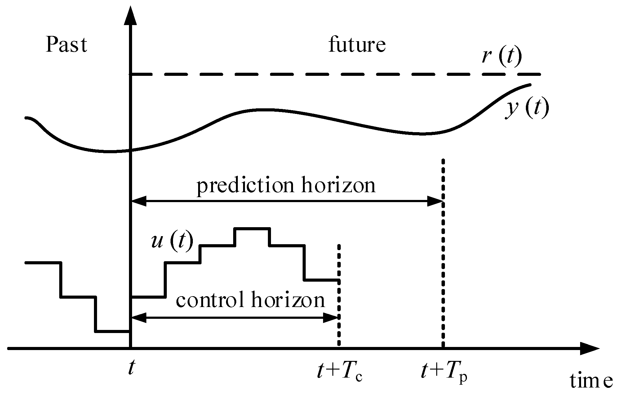
3.1. The Basic Principles of Model Predictive Control (MPC)

The basic principles of MPC can be described as follows: Based on the system prediction model and relevant system information at time $t$, MPC predicts the dynamic behavior of the system over a future time horizon $[t, t+T_{\mathrm{p}}]$. It integrates predefined performance objective functions and associated constraints to solve for a control input sequence $[u(t), u(t+1), \cdots , u(t+T_{\mathrm{c}})]$. This sequence or a portion of it is then applied to the physical system, and the process is repeated at subsequent designed time intervals to seek new control input sequences. Figure 3 illustrates the basic principle of MPC, where $r(t)$ represents the reference trajectory, $y(t)$ denotes the system output, $u(t)$ is the control input, $[t, t+T_{\mathrm{c}}]$ is the control domain, and $[t, t+T_{\mathrm{p}}]$ is the prediction horizon.

Although the models, techniques, and performance requirements employed by MPC vary in practical applications, various types of MPC share common characteristics that can be summarized as follows:

• Prediction model

Because MPC is a model-based predictive method, its application primarily emphasizes the functionality of the chosen model rather than its specific representation. It relies on historical information and current conditions of the system to predict future outputs. For the models used in MPC, as long as they encompass the predictive information relevant to the system, they can serve as predictive models regardless of their specific form. Therefore, the predictive models used in MPC offer considerable flexibility, reducing constraints in the system modeling process and facilitating the advancement of modeling techniques in applications.

2.

Rolling optimization

In comparison with other control theories, MPC exhibits characteristics of rolling optimization and rolling implementation in achieving control actions. In practical engineering applications, MPC often employs online optimization to determine optimal future control inputs by optimizing a specific performance metric within the system. The optimization control in MPC differs significantly from traditional optimal control of discrete systems. In its application, the objective function, which represents desired control performance, typically minimizes the weighted variance between the control output and the desired trajectory. MPC performs online rolling optimization within a finite time horizon at each sampling instant. The performance metric only involves a predefined prediction horizon, which shifts forward accordingly at the next sampling instant.

As the system progresses during operation, the objective function optimizing performance at each sampling instant varies, but their relative forms should remain consistent, and the optimization process continues online and iteratively. Despite the practical limitations in establishing objective functions, which often result in obtaining only locally optimal solutions, this approach effectively compensates for uncertainties caused by model mismatch and disturbances in practical applications. It aims to optimize system performance based on the actual operating state of the system, effectively balancing optimization objectives within the future control horizon and the uncertainties present in the system.

3.

Feedback correction

Feedback correction plays a significant role in overcoming system disturbances, uncertainties, and improving closed-loop stability. Building upon feedback control, MPC complements model predictions through continuous rolling optimization, addressing shortcomings in predictive modeling and mitigating impacts from model mismatch, time-varying dynamics, disturbances, and other factors present in real systems. In MPC optimization, it relies on both the system model and feedback information to form a closed-loop optimization strategy. By compensating for model deficiencies through output feedback under current control actions or modifying predictive models using online identification methods, MPC iteratively applies rolling optimization to correct deviations caused by model mismatch or external disturbances.

4.

Discrete control inputs and explicit constraints

In MPC, the optimization problem essentially involves finding a sequence of control inputs $\{u(t), u(t+1), \cdots , u(t+T-1)\}$ over a time horizon T that ensures the system transitions from an initial state $x_0$ to a final state $x_f$ while optimizing a specified objective function. Continuous control inputs or an infinite time horizon could lead to infinitely many optimal solutions, which increases computational complexity and often results in infeasibility during numerical solutions. Therefore, it is essential to define the optimization problem within a finite time horizon and employ discrete control inputs to ensure stability within each sampling interval. Additionally, MPC explicitly formulates system constraints in open-loop optimization, predicting future conditions to preemptively apply appropriate control actions and prevent system outputs from exceeding specified limits.

3.2. Mixed Logical Dynamical System Predictive Control

The principle of system mixed-logic dynamic modeling involves defining corresponding auxiliary logical variables for different operational states or regions of the system during its operation. Based on the conversion relationship between logical propositions and mixed-integer linear inequalities, the system’s logical expressions, nonlinear terms, and variable constraints are transformed into a linear dynamic system under the form of mixed-integer linear inequalities, typically represented by Equation (3).

3.2.1. Open-Loop Constrained Optimal Control of MLD Models

For an established mixed logical dynamical (MLD) system model, assume its initial state is $x_0$, its terminal time is $T$, and its endpoint is $x_f$. The optimal control objective is to find an optimal control sequence $\{u(0), u(1), \cdots , u(T-1)\}$ such that the system transitions from the initial state $x_0$ to the terminal state $x_f$ at time $T$, while minimizing the following quadratic performance index.

$$\begin{gathered} J={\displaystyle \sum _{t=0}^{T-1}({‖u(t)-u_{\mathrm{f}}‖}_{{\mathrm{Q}}_1}^2}+{‖\delta (t)-{\delta }_{\mathrm{f}}‖}_{{\mathrm{Q}}_2}^2+{‖z(t)-z_{\mathrm{f}}‖}_{{\mathrm{Q}}_3}^2+{‖x(t)-x_{\mathrm{f}}‖}_{{\mathrm{Q}}_4}^2+{‖y(t)-y_{\mathrm{f}}‖}_{{\mathrm{Q}}_5}^2) \\ s. t.\left\{\begin{array}{l}x(T,x_0,u_0^{T-1})=x_{\mathrm{f}}\\ (4-3)\end{array}\right. \end{gathered}$$

(31)

Here, ${‖x‖}_{\mathrm{Q}}^2=x^{\prime }Qx$; $Q_{\mathrm{i}}$ denotes a weighted matrix, and $i\in \left\{1,2,3,4,5\right\}$, while $Q_{\mathrm{i}}=Q_{\mathrm{i}}^{\prime }\ge 0$; $u_f$, ${\delta }_f$, $z_f$, $x_f$, $y_f$ satisfies the inequality constraints specified in (3).

Although (31) does not explicitly include constraints related to state and control inputs, constraints on system states, control inputs, and their interactions are explicitly incorporated in the established MLD model. As indicated by (3), the relationship between system states and inputs is as follows:

$$x(t)=A^{\mathrm{t}}{x}_0+{\displaystyle \sum _{i=0}^{t-1}{A}^{\mathrm{i}}[B_{1}u(t-1-i)+B_2\delta (t-1-i)+B_{3}z(t-1-i)]}$$

(32)

Define the following vector:

$$\mathsf{\Omega }=\left[\begin{array}{c}u(0)\\ u(1)\\ ⋮\\ u(T-1)\end{array}\right], \mathsf{\Delta }=\left[\begin{array}{c}\delta (0)\\ \delta (1)\\ ⋮\\ \delta (T-1)\end{array}\right], \mathsf{\Xi }=\left[\begin{array}{c}z(0)\\ z(1)\\ ⋮\\ z(T-1)\end{array}\right], \gamma =\left[\begin{array}{c}\mathsf{\Omega }\\ \mathsf{\Delta }\\ \mathsf{\Xi }\end{array}\right]$$

Mixed-integer quadratic programming (MIQP) offers relative ease of solution, and when the weighted matrix is positive definite, the quadratic performance index optimization control problem has a unique solution. Moreover, the weighted matrix has a clear physical meaning. By substituting (32) into (31) and (3), the open-loop optimal control problem for the mixed logical dynamical system can be transformed into the following standard MIQP problem.

$$\begin{array}{l}\underset{\gamma }{\min } 0.5{\gamma }^{\prime }H\gamma +F\gamma \\ s. t.\left\{\begin{array}{l}{A}_{\mathrm{ineq}}\gamma \le b_{\mathrm{ineq}}\\ A_{\mathrm{eq}}\gamma =b_{\mathrm{eq}}\\ \gamma \in R^{\mathrm{nc}}\times {\{0,1\}}^{\mathrm{nd}}\\ \gamma (itype)\in {\{0,1\}}^{\mathrm{nd}}\end{array}\right.\end{array}$$

(33)

Here, $H>0$; $\gamma$ represents the decision vector, and $\gamma (itype)$ denotes the binary logical elements specified in $\gamma$.

By solving (33), the optimal control sequence that satisfies the performance index (31) can be obtained. When the MLD model of the system (3) includes $D_1=D_2=D_3=0$, we have:

$$H=\tilde{Q}+{\displaystyle \sum _{t=1}^{T-1}{A}_{\mathrm{B}}^{\prime }(t)(Q_4+C^{\prime }{Q}_{5}C)A_{\mathrm{B}}(t)}$$

(34)

$$F=-{\gamma }_{\mathrm{f}}^{\prime }\tilde{Q}-{\displaystyle \sum _{t=1}^{T-1}(-x_{\mathrm{f}}^{\prime }{Q}_4+y_{\mathrm{f}}^{\prime }{Q}_{5}C)A_{\mathrm{B}}(t)}+x_0^{\prime }{\displaystyle \sum _{t=1}^{T-1}{A}_{\mathrm{B}}^{\prime }(t)(Q_4+C^{\prime }{Q}_{5}C)A_{\mathrm{B}}(t)}$$

(35)

Here:

$$\left\{\begin{array}{l}\tilde{Q}=diag(Q_1, Q_2, Q_3)\\ Q_{\mathrm{i}}=diag(Q_{\mathrm{i}}, Q_{\mathrm{i}}, \cdots , Q_{\mathrm{i}}{)}_{\mathrm{T}\times \mathrm{T}},\hspace{1em}i=1, 2, 3\\ A_{\mathrm{B}}(t)=[A_{\mathrm{B}1}(t) A_{\mathrm{B}2}(t) A_{\mathrm{B}3}(t)]\\ A_{\mathrm{Bi}}(t)=[A^{T-1}{B}_{\mathrm{i}} A^{T-2}{B}_{\mathrm{i}} \cdots A{B}_{\mathrm{i}} B_{\mathrm{i}} 0 \cdots 0{]}_{1\times \mathrm{T}}\end{array}\right.$$

(36)

$$A_{\mathrm{eq}}=A_{\mathrm{B}}^{\left(\mathrm{T}\right)}, b_{\mathrm{eq}}=x_{\mathrm{f}}-A^{\prime }{x}_0$$

(37)

$$A_{\mathrm{ineq}}=\left[\begin{array}{ccc}\widetilde{E_1^{(0)}}& \widetilde{E_2^{(0)}}& \widetilde{E_3^{(0)}}\\ \widetilde{E_1^{(1)}}& \widetilde{E_2^{(1)}}& \widetilde{E_3^{(1)}}\\ ⋮& ⋮& ⋮\\ \widetilde{E_1^{(T-1)}}& \widetilde{E_2^{(T-1)}}& \widetilde{E_3^{(T-1)}}\end{array}\right], b_{\mathrm{ineq}}=\left[\begin{array}{c}{E}_4\\ E_{4}A\\ ⋮\\ E_4{A}^{T-1}\end{array}\right]x_0+\left[\begin{array}{c}{E}_5\\ E_5\\ ⋮\\ E_5\end{array}\right]$$

(38)

$$\widetilde{E_1^{(t)}}={\left[\begin{array}{ccccccccc}-E_4{A}^{t-1}{B}_1& -E_4{A}^{t-2}{B}_1& \cdots & -E_{4}A{B}_1& -E_4{B}_1& -E_1& 0& \cdots & 0\end{array}\right]}_{1\times \mathrm{T}}$$

(39)

$$\widetilde{E_{\mathrm{j}}^{(t)}}={\left[\begin{array}{ccccccccc}-E_4{A}^{t-1}{B}_{\mathrm{j}}& -E_4{A}^{t-2}{B}_{\mathrm{j}}& \cdots & -E_{4}A{B}_{\mathrm{j}}& -E_4{B}_{\mathrm{j}}& -E_{\mathrm{j}}& 0& \cdots & 0\end{array}\right]}_{1\times \mathrm{T}}$$

(40)

$$\widetilde{E_1^{\left(0\right)}}={\left[-\begin{array}{cccc}{E}_1& 0& \cdots & 0\end{array}\right]}_{1\times \mathrm{T}}$$

(41)

$$\widetilde{E_{\mathrm{j}}^{\left(0\right)}}={\left[\begin{array}{cccc}{E}_{\mathrm{j}}& 0& \cdots & 0\end{array}\right]}_{1\times \mathrm{T}}$$

(42)

And, $1\le t\le T-1, j=2, 3$.

Currently, solving mixed-integer quadratic programming (MIQP) problems primarily involves methods such as the Cutting Plane Method [22], Decomposition Method [23], evolutionary algorithms [24], and Branch & Bound [25,26,27]. Among these, Branch & Bound is particularly effective for moderately sized MIQP problems. This method essentially treats the process of solving the MIQP problem as a search through a binary tree. By relaxing some or all of the binary integer constraints in the decision variables $\gamma$, each node in the binary tree is transformed into a quadratic programming (QP) problem corresponding to that node. Solving these QP problems recursively provides a globally optimal solution or suboptimal solutions that satisfy the integer constraints.

Assuming $\xi$ is a vector of the same dimension as the binary integer constraints in $\gamma$. For an MIQP problem, relaxing all binary integer constraints in $\gamma$ yields:

$${\xi }_0={[\begin{array}{cccc}\ast & \ast & \cdots & \ast \end{array}]}_{1\times \mathrm{nd}}$$

(43)

Here, $\ast$ as any real number between [0, 1].

Solve the relaxed $\gamma$ QP problem to obtain the optimal decision variables ${\gamma }_{\mathrm{opt}}$ and the optimal value $f_{\mathrm{opt}}$. If the problem is infeasible or its $f_{\mathrm{opt}}=\infty$, then the original MIQP problem is also infeasible. If the obtained ${\gamma }_{\mathrm{opt}}$ is 0 or 1, then ${\gamma }_{\mathrm{opt}}$ is the global optimal solution for the original MIQP problem. If ${\gamma }_{\mathrm{opt}}$ does not satisfy the binary integer constraints, two new sub-QP problems corresponding to Formula (44) are generated. This process is repeated until the preset maximum number of QP problem solutions is reached. Figure 4 shows the binary tree for solving an MIQP problem with two binary integer constraints using the Branch & Bound method.

$${\xi }_1={[\begin{array}{cccc}1& \ast & \cdots & \ast \end{array}]}_{1\times \mathrm{nd}},\hspace{1em}{\xi }_2={[\begin{array}{cccc}0& \ast & \cdots & \ast \end{array}]}_{1\times \mathrm{nd}}$$

(44)

3.2.2. Model Predictive Control of MLD Systems

Since the control input sequence for open-loop optimal control of mixed logical dynamical (MLD) systems is obtained through discrete computation, the controller has poor robustness and ability to respond to system disturbances. Additionally, when the system is large-scale, has many state variables, or has a long control horizon, the computational complexity increases significantly, making the problem difficult to solve. The essence of model predictive control (MPC) is to use a receding horizon control approach to solve the optimal control problem online, effectively handling system constraints during the optimization process and improving the controller’s ability to cope with system uncertainties.

The basic principle of model predictive control (MPC) based on the mixed logical dynamical (MLD) model involves establishing the MLD model for the control input $U_{dc}$ (DC bus voltage value) of the controlled system and using this model as the predictive model for MPC. A cost function is then formulated for rolling optimization. During the rolling optimization process, auxiliary logical variables are introduced in the MLD model, allowing the optimization problem to be transformed into a Mixed-Integer Quadratic Programming (MIQP) or Mixed-Integer Linear Programming (MILP) problem. The goal is to find the first element of the control sequence that minimizes the cost function and apply it to the controlled system, ensuring that the system’s output tracks the reference trajectory under the influence of the control input. This process is repeated at the next time step to continuously solve for the control input (while keeping it within preset upper and lower threshold limits $U_{dc\_H}$). The basic principle is illustrated in Figure 5.

Model predictive control (MPC) is an optimization control algorithm that uses a specific objective function as a criterion within a finite future horizon. Its implementation process involves specific optimization performance indices at each sampling instant, rather than using a globally identical optimization objective function. The time horizons included in the optimization performance indices at different times also vary. The optimization process is carried out repeatedly online, determining the future control input sequence $\{u(k\left|t\right.), u(k+1\left|t\right.), \cdots , u(k+p\left|t\right.)\}$ within the prediction horizon at time t according to the objective function criterion. Each time, only the first element $u(k\left|t\right.)$ of the obtained optimal control sequence is applied to the control process using the rolling optimization method. This is the fundamental difference between MPC and traditional optimal control.

Assume $x(k\left|t\right.)$ represents the predicted result at time $t+k$ under the influence of $u_{\mathrm{t}}^{\mathrm{k}-1}$ at time $t$, and $y(k\left|t\right.)$, $\delta (k\left|t\right.)$, $z(k\left|t\right.)$ are defined similarly. Define $(x_{\mathrm{e}}, u_{\mathrm{e}})$ as the system equilibrium point, $({\delta }_{\mathrm{e}}, z_{\mathrm{e}})$ as the corresponding auxiliary variable, and $u_{\mathrm{t}}^{\mathrm{T}-1}=\{u(0), u(1), \cdots , u(T-1)\}$ as the control sequence at time $t$.

Assume at time $t=0$, $x(0)$ is the initial state, and consider the following quadratic performance index optimization problem:

$$\begin{array}{l}\underset{\left\{u_0^{\mathrm{T}-1}\right\}}{\min }J(u_0^{\mathrm{T}-1},x(t))={\displaystyle \sum _{k=0}^{T-1}({‖u(t)-u_{\mathrm{e}}‖}_{{\mathrm{Q}}_1}^2}+{‖\delta (\left.k\right|t)-{\delta }_{\mathrm{e}}‖}_{{\mathrm{Q}}_2}^2\\ \hspace{1em}\hspace{1em}\hspace{1em}\hspace{1em}\hspace{1em}\hspace{1em}\hspace{1em}+{‖z(\left.k\right|t)-z_{\mathrm{e}}‖}_{{\mathrm{Q}}_3}^2+{‖x(\left.k\right|t)-x_{\mathrm{e}}‖}_{{\mathrm{Q}}_4}^2+{‖y(\left.k\right|t)-y_{\mathrm{e}}‖}_{{\mathrm{Q}}_5}^2)\\ \hspace{1em}\hspace{1em}\hspace{1em}s. t.\left\{\begin{array}{l}x(T\left|t\right.)=x_{\mathrm{e}}\\ (4-3)\\ u_{\min }\le u(k\left|t\right.)\le u_{\max }, k=0, 1, \cdots , T-1\\ x_{\min }\le x(k\left|t\right.)\le x_{\max }, k=0, 1, \cdots , T-1\\ y_{\min }\le y(k\left|t\right.)\le y_{\max }, k=0, 1, \cdots , T-1\end{array}\right.\end{array}$$

(45)

Similar to optimal control, the above problem can ultimately be transformed into an MIQP problem for solution. During each implementation of the rolling optimization process, only the first element $u_{\mathrm{t}}^{*}(0)$ of the current optimal control sequence $u_{\mathrm{t}}^{*}={\{u_{\mathrm{t}}^{*}(k)\}}_{\mathrm{k}=0, 1, \cdots , \mathrm{T}-1}$ is applied to the system.

Model predictive control fundamentally involves solving constrained finite-horizon optimization problems iteratively. Its open-loop optimal solution does not guarantee closed-loop stability. Due to the complex nature of mixed logical dynamical systems, deriving closed-loop equations is challenging. To ensure stability in predictive control, additional constraints are commonly added to guarantee closed-loop stability of the control algorithm. Therefore, stability analysis of MPC for MLD models is essential. For systems based on finite-horizon predictive control, introducing terminal constraints allows using the optimal performance index function as the Lyapunov function for MPC control algorithms. The monotonic decrease in the performance index demonstrates the Lyapunov stability of the system.

3.3. Model Predictive Control of Microgrid Systems with MLD Models

To verify the accuracy of the proposed energy management strategy, a microgrid experimental platform was set up as shown in Figure 6 To ensure the reliability of the experiment, a Chroma 62150H-600S (Chroma ATE, Taiyuan, China) was used to simulate the photovoltaic array, while a Taiwan Kikusui ACLT-3803M (Taiwan Kikusui Co., Ltd., Taipei, China) was used as the load. The testing equipment included a Yokogawa DL850 oscilloscope (Yokogawa Electric Corporation, Tokyo, Japan). Figure 6 shows a photograph of the experimental platform constructed for this study.

According to Section 2.3, the DC bus energy $E_{dc}$ from photovoltaic generation units is considered as the system state variable. Based on the relationship between the DC bus voltage and $E_{dc}$, the switching conditions for energy storage unit charge/discharge are designed. The charge/discharge states of the storage unit are equivalently represented as binary logic ‘0,1’. Under each logic state, the operation of each unit in the system can be seen as continuous dynamic events. Therefore, a microgrid is a typical hybrid system that can be described by establishing an MLD model to depict its operational states and achieve optimized control through MPC.

For the microgrid MLD mechanistic model established by Equations (29) and (30), assuming the DC bus voltage thresholds for storage unit state transitions are 420 V and 380 V, corresponding to energies $M_{dc}=82.908J$ and $m_{dc}=67.868J$, respectively, the DC bus voltage protection limits are set at 450 V and 360 V, corresponding to energies $E_{\max }=95.175J$ and $E_{\min }=60.912J$. The control performance curve of the microgrid system is depicted in Figure 7. Here, $P_{array}$ represents the output power of the photovoltaic array, and $\delta$ denotes the operation state of the energy storage unit, where $\delta =1$ signifies the discharge process and $\delta =0$ denotes the charge process.

Based on the simulation results, it is evident that the microgrid system MLD mechanistic model developed in this study effectively reflects the operational state of the microgrid during fluctuations in photovoltaic array output power and load. By adjusting the operational states of the energy storage unit and input/output power, the MLD model indirectly adjusts the system control inputs to maintain energy balance. During simulation, the photovoltaic array output power fluctuated randomly, with the load increasing from 1740 W to 2225 W at 0.5 s, 3.5 s, 4.5 s, 6 s, and 8.5 s, and decreasing from 2225 W to 1740 W at 3 s, 4 s, 5.5 s, 6.5 s, and 9 s. The maximum DC bus voltage of the photovoltaic unit was 440.4481 V, and the minimum was 361.2084 V. Based on the relationship between capacitor voltage and instantaneous energy, the system control error was determined to be 9.97%. The energy storage unit switched states a total of 91 times.

Figure 8 presents the simulated outputs of various units in the microgrid system derived from the MLD model. The load increases at 0.07 s and decreases at 0.12 s, while the output power of the photovoltaic array fluctuates randomly due to external conditions. According to the principles of the MLD model, the energy storage unit operates in discharge mode from 0 to 0.05 s and from 0.09 s to 0.15 s, and in charge mode from 0.05 s to 0.09 s and from 0.15 s to 0.2 s. The system’s output voltage and current waveforms are smooth with no abrupt transitions.

Based on optimal control and model predictive control theory, and using the microgrid system MLD model as a foundation, design a tracking-type performance index (46). In this index, the first term aims to stabilize the DC bus voltage of the photovoltaic unit, while the second term aims to minimize the number of state transitions in the energy storage unit. Assuming a system weight matrix $S_1=S_2=1$, design target values for the charge/discharge process outputs as 82.908 J and 67.868 J (corresponding to 420 V and 380 V).

$$\begin{array}{l}\min J(\delta (t),x(t))={\displaystyle \sum _{k=0}^{T-1}(S_1{‖y(\left.k\right|t)-y_{\mathrm{e}}‖}^2}+S_2{‖{\delta }_3(\left.k\right|t)-{\delta }_4(\left.k\right|t)‖}^2)\\ \hspace{1em}\hspace{1em}\hspace{1em}s. t.\left\{\begin{array}{l}x(T\left|t\right.)=x_{\mathrm{e}}\\ (4-3)\\ u_{\min }\le u(k\left|t\right.)\le u_{\max }, k=0, 1, \cdots , T-1\\ x_{\min }\le x(k\left|t\right.)\le x_{\max }, k=0, 1, \cdots , T-1\\ y_{\min }\le y(k\left|t\right.)\le y_{\max }, k=0, 1, \cdots , T-1\end{array}\right.\end{array}$$

(46)

Figure 9 shows the simulation results of the model predictive control-based microgrid system designed using the performance index (46). Under the same input conditions as the MLD mechanistic model, the maximum DC bus voltage of the photovoltaic unit is 439.122 V, and the minimum is 360.8653 V. According to the relationship between capacitor voltage and instantaneous energy, the system control error is determined to be 9.81%. The energy storage unit switched states a total of 41 times. A comparison reveals that the model predictive control method effectively suppresses fluctuations in the DC bus voltage while reducing the number of charge/discharge cycles of the energy storage unit, thereby enhancing battery lifespan and system cost-effectiveness.

Figure 10 displays the output waveforms of each unit based on model predictive control. The load increases at 0.04 s and decreases at 0.14 s, while the output power of the photovoltaic array fluctuates randomly. The system achieves effective control of output voltages and currents for each unit.

4. Conclusions

This paper, based on energy management processes, analyzes the hybrid characteristics of microgrid operations. By comparing and analyzing the characteristics and advantages/disadvantages of existing modeling approaches for hybrid systems, a mixed logical dynamic model of microgrid systems is established. Incorporating optimal control and model predictive control theories with the goal of reducing fluctuations in the DC bus voltage of photovoltaic units and minimizing charge/discharge cycles of energy storage devices, especially when distributed power generation and load variations are minimal, this method effectively suppresses DC bus voltage fluctuations. Simulation results validate the correctness of the proposed approach. The study outcomes provide a basis for designing energy management strategies in subsequent phases.

References

1. Golestani, S.; Tadayon, M. Distributed generation dispatch optimization by artificial neural network trained by particle swarm optimization algorithm. In Proceedings of the 8th International Conference on the European Energy Market, Zagreb, Croatia, 25–27 May 2011; pp. 543–548. [Google Scholar]
2. Wang, X.; Zhang, C. Seamless Switching Control Strategy for Distributed Generation Systems. Trans. China Electrotech. Soc. 2012, 27, 218–222. [Google Scholar]
3. Katiraei, F.; Iravani, M.R. Power Management Strategies for a Microgrid with Multiple Distributed Generation Units. IEEE Trans. Power Syst. 2006, 21, 1821–1831. [Google Scholar] [CrossRef]
4. Li, Y.W.; Kao, C. An accurate power control strategy for inverter based distributed generation units operating in a low voltage microgrid. In Proceedings of the Energy Conversion Congress and Exposition, San Jose, CA, USA, 20–24 September 2009; pp. 3363–3370. [Google Scholar]
5. Miao, Y.; Cheng, H.; Gong, X. Discussion on Distribution Network Connection Modes with Microgrids. Proc. CSEE 2012, 32, 17–23. [Google Scholar]
6. Tan, K.T.; So, P.L.; Chu, Y.C. Control of parallel inverter-interfaced distributed generation systems in microgrid for islanded operation. In Proceedings of the 11th International Conference on Probabilistic Methods Applied to Power Systems, Singapore, 14–17 June 2010; pp. 1–5. [Google Scholar]
7. Majumder, R.; Chakrabarti, S.; Ledwich, G.; Ghosh, A. Control of battery storage to improve voltage profile in autonomous microgrid. In Proceedings of the Power and Energy Society General Meeting, Detroit, MI, USA, 24–28 July 2011; pp. 1–8. [Google Scholar]
8. Zheng, K.-H.; Xia, M.-C. Impacts of microgrid on protection of distribution networks and protection strategy of microgrid. In Proceedings of the International Conference on Advanced Power System Automation and Protection, Beijing, China, 16–20 October 2011; pp. 356–359. [Google Scholar]
9. Lasseter, R.H.; Eto, J.H.; Schenkman, B. CERTS Microgrid Laboratory Test Bed. IEEE Trans. Power Deliv. 2011, 26, 325–332. [Google Scholar] [CrossRef]
10. Erickson, M.J.; Jahns, T.M.; Lasseter, R.H. Comparison of PV inverter controller configurations for CERTS microgrid applications. In Proceedings of the IEEE Energy Conversion Congress and Exposition, Phoenix, AZ, USA, 17–22 September 2011; pp. 659–666. [Google Scholar]
11. Su, W.; Yuan, Z.; Chow, M.Y. Microgrid planning and operation: Solar energy and wind energy. In Proceedings of the IEEE Power and Energy Society General Meeting, Providence, RI, USA, 25–29 July 2010; pp. 1–7. [Google Scholar]
12. Zhang, J.; Huang, W. Microgrid Operation Control and Protection Technologies; Electric Power Press: Beijing, China, 2010; pp. 22–25. [Google Scholar]
13. Morozumi, S.; Kikuchi, S.; Chiba, Y.; Kishida, J.; Uesaka, S.; Arashiro, Y. Distribution technology development and demonstration projects in Japan. In Proceedings of the IEEE Power and Energy Society General Meeting, Pittsburgh, PA, USA, 20–24 July 2008; pp. 1–7. [Google Scholar]
14. Peng, L.; Ling, Z.; Wei, W. Application and Analysis of Microgrid Technology. Autom. Electr. Power Syst. 2009, 33, 109–115. [Google Scholar]
15. Ma, H.; Feng, Q.; Guo, J. Boost-Type DC/DC Switching Converter Hybrid Modeling and Control Research. J. China Railw. Soc. 2010, 32, 50–55. [Google Scholar]
16. Zheng, X.; Li, C.; Rong, Y. Hybrid System Modeling and Predictive Control of DC/AC Converters. Trans. China Electrotech. Soc. 2009, 24, 87–92. [Google Scholar]
17. Li, X.; Zhou, D. Fault Diagnosis of Power Electronic Circuits Based on Hybrid Model and Filter. J. Northwest Univ. 2011, 41, 410–414. [Google Scholar]
18. Ma, H.; Mao, X.; Xu, D. Parameter Identification of DC/DC Power Electronic Circuits Based on Hybrid System Model. Proc. Chin. Soc. Electr. Eng. 2005, 25, 50–54. [Google Scholar]
19. Mo, Y.; Xiao, D. Review on Hybrid Dynamical Systems and Their Applications. Control Theory Appl. 2002, 19, 1–8. [Google Scholar]
20. Wang, G.; Song, J. Quantification Methods in Propositional Logic. Acta Electron. Sin. 2006, 34, 252–257. [Google Scholar]
21. Ekaputri, C.; Syaichu-Rohman, A. Implementation model predictive control (MPC) algorithm for inverted pendulum. In Proceedings of the IEEE Control and System Graduate Research Colloquium, Shah Alam, Malaysia, 16–17 July 2012; pp. 116–122. [Google Scholar]
22. Kong, F.W.; Kuhn, D.; Rustem, B. A cutting-plane method for Mixed-Logical Semidefinite Programs with an application to multi-vehicle robust path planning. In Proceedings of the IEEE 49th Conference on Decision and Control, Atlanta, GA, USA, 15–17 December 2010; pp. 1360–1365. [Google Scholar]
23. Sakawa, M.; Kato, K.; Mohara, H. Efficiency of a decomposition method for large-scale multiobjective fuzzy linear programming problems with block angular structure. In Proceedings of the 2nd International Conference on Knowledge-Based Intelligent Electronic Systems, Adelaide, Australia, 21–23 April 1998; pp. 80–86. [Google Scholar]
24. Zhuo, K.; Yan, L.; Bo, L. A general evolutionary algorithm for mixed-integer nonlinear programming problems. J. Comput. Res. Dev. 2002, 39, 1471–1477. [Google Scholar]
25. Zhang, J.; Li, P.; Wang, W. Solving and Application of MIQP Problems Based on the Branch & Bound Method. J. Syst. Simul. 2003, 15, 488–491. [Google Scholar]
26. Wang, L.; Hao, G. Drainage pipe network optimization design based on branch-bound method. In Proceedings of the 2nd International Conference on Intellectual Technology in Industrial Practice, Changsha, China, 8–9 September 2010; pp. 260–263. [Google Scholar]
27. Qie, Z.; Shang, F. An algorithm for indefinite quadratic programming over an unbounded domain. J. Shenyang Jianzhu Univ. 2001, 17, 75–80. [Google Scholar]
Figure 1. Structural composition of the designed microgrid.
Energies 17 04285 g001
Figure 2. The diagram of hybrid model for microgrid.
Energies 17 04285 g002
Figure 3. The principle of model predictive control.
Energies 17 04285 g003
Figure 4. The binary tree of MIQP with two integral constraints.
Energies 17 04285 g004
Figure 5. The diagram of MLD predictive model with feedback control.
Energies 17 04285 g005
Figure 6. The test platform of proposed microgrid.
Energies 17 04285 g006
Figure 7. Simulation results of the microgrid based on MLD model.
Energies 17 04285 g007
Figure 8. Output waveforms of subsystems based on MLD model.
Energies 17 04285 g008
Figure 9. Simulation results based on model predictive control.
Energies 17 04285 g009
Figure 10. Output waveforms of subsystems based on model predictive control.
Energies 17 04285 g010