Investigation of a Fuel-Flexible Diffusion Swirl Burner Fired with NH₃ and Natural Gas Mixtures

Abstract

The current investigation aims to develop a validated numerical model of a confined, swirl-stabilized diffusion flame. This model will assist in designing and optimizing novel combustion chambers while reducing computational costs. To achieve this objective, experimental and numerical studies were conducted on NH₃/natural gas combustion using a laboratory-scale burner capable of operating under fuel-flexible conditions. The burner fired 5 kW flames of blended ammonia with natural gas in concentrations up to 100% NH₃. The burner’s performance for relevant industrial applications was assessed through measurements of axial temperature profiles, exhaust temperature, and gas emissions. Numerical simulations were conducted by employing the commercial CFD software STAR-CCM+ 2020.2.1. Numerical simulations for steady-state were performed using a realizable k-$ϵ$ turbulence model coupled with the EDC (eddy dissipation concept) for combustion. The investigation utilized a 3D periodic domain for the simulations and investigated mesh independence and the influence of the flame dynamics. The burner was able to operate with different fuel mixtures while maintaining stabilized flames under every condition. However, the appearance of increased ammonia slip was observed for 100% NH₃ up to 1250 ppm (dry vol.). The present work demonstrates and assesses the readiness and potential of fuel-flexible burners as cost-effective and efficient transitional technologies for integrating ammonia and other sustainable fuels into combustion applications.

1. Introduction

The escalating issue of environmental concerns arising from the excessive emission of greenhouse gases and pollutants has garnered significant attention from governmental, research, and industrial entities. A notable illustration of this paradigm shift is the Paris Agreement (2012), which aimed to mitigate greenhouse gas emissions and reduce the global temperature rise to below 2 °C by the end of the century. The European Union (EU) and various other nations have made a resolute commitment to implement substantial decarbonization measures. These measures aim to achieve climate neutrality by 2050 and to create an economy that maintains a net-zero level of greenhouse gas emissions. This objective forms the core of the European Green Deal and aligns harmoniously with the EU’s dedication to international climate action in accordance with the Paris Agreement [1]. Consequently, immediate and concerted actions are imperative, with specific emphasis placed on the energy and industrial sectors, known as the primary contributors of CO₂ emissions. Therefore, disruptive technologies are necessary to achieve substantial emission reductions within a strict timeline. Ammonia, as a carbon-free fuel, has emerged as a potential candidate for a revolutionary fuel source in future energy systems [2,3]. In 2020, the worldwide ammonia production capacity was 224 million tonnes (Mt), ranking it as the ninth most-produced chemical globally. Currently, ammonia is made from fossil fuel–derived hydrogen and is therefore not a “green” product, despite its widespread use in agriculture. However, environmentally green ammonia may be on the horizon if the hydrogen is made by other means, such as wind or solar-powered water electrolysis [4]. The prominence of green ammonia as a central component within the hydrogen economy extends beyond its relevance to the energy sector. Its potential also lies in its capacity to mitigate emissions in various other industries.

Ammonia possesses notable attributes, including a high energy density and the capability to be stored in liquid form at ambient temperature and relatively low pressures (as low as 10 bars). Moreover, it exhibits lower risks of explosion or flashback compared to other gaseous fuels due to its relatively low reactivity. Employing ammonia directly as a fuel presents certain challenges, as its combustion performance and emission characteristics require new approaches and strategies. As previously mentioned, these challenges arise from ammonia’s low laminar flame speed, peaking at approximately 7 cm/s under room conditions with a fuel/air equivalence ratio of 1.1. Natural gas exhibits much broader combustion characteristics, with a peak laminar flame speed of approximately 37.4 cm/s. Ammonia demonstrates extended ignition delay times and a limited flammability range, with equivalence ratios of 0.63–1.4, compared to natural gas, which has a broader flammability range of 0.5–1.7 in terms of its equivalence ratio. To address its limited flammability properties, blending ammonia with a more reactive fuel, such as hydrogen or methane, is recommended for various applications [2,3,5].

In terms of emissions, ammonia presents certain drawbacks when compared to natural gas. When burned under lean or stoichiometric conditions, it produces elevated levels of NO_x emissions. The presence of ammonia in flue gas due to incomplete combustion poses an additional concern in practical combustion systems due to its toxicity and corrosive nature, particularly with respect to copper-containing alloys. Another significant aspect that has yet to be extensively explored is the formation of N₂O, an exceedingly potent greenhouse gas approximately 265 times more impactful than CO₂ [6]. Okafor et al. [7] have addressed this subject, highlighting the detection of N₂O formation near walls, where incomplete combustion occurs at lower temperatures. N₂O is a potential byproduct of ammonia combustion and after-treatment technologies. Even small amounts of N₂O can lead to high GHG emissions, which can be a potential obstacle to using ammonia as a low-emission alternative fuel. Consequently, small quantities of N₂O may invalidate the use of ammonia as a low-emission fuel. This highlights the importance of studying combustion technologies that minimize N₂O production in ammonia combustion applications [6].

Regarding gas turbines, despite notable advancements, particularly highlighted in the works of Okafor et al. [8,9], the majority of burners utilized in ammonia studies within the literature were initially designed for other fuels, such as kerosene or methane. Further investigations conducted by Okafor et al.’s research group discovered that lean conditions in conventional swirl burners led to substantial production of NO_x and NH₃ slip. Additionally, the authors extended their research to dual-fuel ammonia/methane flames and observed a comparable positive performance. Recent studies [10] have examined the oxidation characteristics of CH₄/NH₃ mixtures, revealing that reactivity occurs at lower temperatures when compared to pure methane in cases where NH₃ constitutes less than 40% of the fuel mixture. This suggests that low concentrations of NH₃ exert a promoting effect on the reactivity of the mixture. However, as the NH₃ concentration increases, the enhancing effect becomes less pronounced, ultimately vanishing for NH₃ concentrations exceeding 50%. Furthermore, the ignition of such mixtures occurs at higher inlet temperatures in comparison to pure methane. Cheng et al. [11] studied the explosion characteristics of fuel mixtures for the laminar combustion of ammonia–air and ammonia–oxygen mixtures. The study reported that an equivalence ratio of 0.8 presented the lowest pressure rise for tests performed at ambient pressure. Cheng et al. [12] also studied ammonia–hydrogen–air explosion characteristics and flame speed. They observed that the addition of NH₃ led to a reduction in the maximum explosion pressure achieved after ignition and in the explosion time to reach peak pressure, leading to a lower maximum explosion rise rate. The addition of hydrogen led to a lower activation energy and a broader flammability range when compared to pure ammonia tests. This investigation highlights the potential for combustion applications to operate under multi-fuel conditions, which can mitigate the flammability and ignition limitations of ammonia combustion while reducing the risk and impact of explosions on premixed combustion applications.

The aforementioned findings support the potential implementation of ammonia combustion systems operating under dual-fuel conditions. Consequently, the integration of ammonia represents a prospective strategy for reducing greenhouse gas emissions in the near future, with relatively cost-effective and expedient implementation during a transitional period. Figure 1 highlights the potential of ammonia production, distribution, and use in a CO₂-free valuable chain, which could be used for energy production via direct combustion or in a fuel cell. Additionally, green ammonia might be used as a feedstock in other industries (for example, the chemical and agricultural industries).

In this context, the present study aims to build upon previous investigations by firing a swirl burner with mixtures of NH₃ and Natural Gas and conducting numerical simulations of the combustor operation using 3D periodic Computational Fluid Dynamics (CFD) Reynolds-Averaged Navier–Stokes (RANS) modeling. The simulations were performed using a fine mesh to capture the geometric details and flowfield, incorporating a detailed kinetic mechanism. This research seeks to advance the understanding of ammonia combustion applications, enabling a versatile and adaptable combustion process that can be rapidly implemented to reduce dependence on fossil fuels. The dual-fuel flexible operation (0–100 % NH₃) offers the potential to retrofit conventional combustion applications, such as boilers and furnaces in hard-to-abate sectors, providing a viable solution for reducing CO₂ emissions during the transition toward sustainable energy sources. Although a few works on NH₃ blended fuel have been published, they are mostly focused on premixed combustion regimes [13,14] for gas turbine applications. The present work is concerned with diffusion flame burners, which are more commonly available in industrial applications. Moreover, this investigation explores a computationally efficient model for evaluating the flow field and operational characteristics associated with ammonia combustion. The numerical model aims to predict the impact of adding NH₃ to combustion applications in a cost-effective manner, thus enabling broader adoption and faster implementation of cleaner energy solutions.

2. Numerical Model

2.1. Governing Equations for Reactive Fluid Flow

The Reynolds Averaged Navier–Stokes (RANS) equations consist of the continuity (1a) and momentum (1b) equations. Additionally, in a reactive flow scenario, the energy conservation equation is also required (1c). They are presented as follows in both their compressible and conservative forms:

$${\displaystyle \frac{\partial \overline{\rho }}{\partial t}}+\nabla ·\left(\overline{\rho }\overline{u}\right)=0$$

(1a)

$$\begin{array}{c}\hfill {\displaystyle \frac{\partial }{\partial t}}\left(\overline{\rho }\overline{u}\right)+\nabla ·\left(\overline{\rho }\overline{u}\overline{u}\right)=-\nabla \overline{p}+\left(\nabla ·\left(\overline{\tau }-\overline{\rho u^{\prime }{u}^{\prime }}\right)\right)+\overline{f_b}\end{array}$$

(1b)

$$\begin{array}{c}\hfill {\displaystyle \frac{\partial }{\partial t}}\left(\overline{\rho }{c}_p\overline{T}\right)+\nabla ·\left(\overline{\rho }{c}_p\overline{u}\overline{T}\right)=\nabla ·\left(K\nabla \overline{T}-C_p\overline{\rho u^{\prime }{T}^{\prime }}\right)+\overline{S^T}\end{array}$$

(1c)

where u is the velocity vector, $\rho$ is the density, p is the pressure, $C_p$ represents the specific heat capacity at constant pressure, K is the thermal conductivity of the fluid, $\tau$ is the viscous stress tensor, T is the temperature, $f_b$ is the body forces, $\overline{\rho u^{\prime }{u}^{\prime }}$ is the Reynolds stress tensor, $\overline{\rho u^{\prime }{T}^{\prime }}$ is the turbulent scalar flux, and $S^T$ represents the energy source term due to combustion and radiation.

2.2. Turbulent Closure-Realizable k-$ϵ$ Model

The realizable k-$ϵ$ model is a widely used turbulence model in computational fluid dynamics (CFD) for simulating turbulent flows. It improves upon the standard k-$ϵ$ model by addressing some of its limitations, providing more accurate and reliable predictions for a broader range of flow types. This model is more suitable for flows with strong swirling effects, such as those encountered in the present work. The realizable model accounts for the effects of mean rotation in a more accurate way.

The realizable k-$ϵ$ model contains a modified transport equation for the turbulent dissipation rate $ϵ$ [15]. Also, a variable damping function $F_{\mu }$ expressed as a function of mean flow and turbulence properties is applied to a coefficient of the model $C_{\mu }$. This procedure ensures that the model satisfies certain mathematical constraints on the normal stresses, consistent with the physics of turbulence (realizability). This concept of a damped $C_{\mu }$ is also consistent with experimental observations in boundary layers.

The turbulent kinetic energy (k) equation can be written as:

$${\displaystyle \frac{\partial \left(\overline{\rho }k\right)}{\partial t}}+\nabla ·\left(\overline{\rho }\overline{u}k\right)=\nabla ·\left[\left(\mu +{\displaystyle \frac{{\mu }_t}{{\sigma }_k}}\right)\nabla k\right]+P_k-\rho ϵ$$

(2)

where $\mu$ is the dynamic viscosity, ${\mu }_t$ is the turbulent viscosity, ${\sigma }_k$ is the turbulent Prandtl number for k, $P_k$ is the production term of turbulent kinetic energy, and $ϵ$ is the dissipation rate of turbulent kinetic energy. The dissipation rate ($ϵ$) equation can be defined as follows:

$${\displaystyle \frac{\partial \left(\rho ϵ\right)}{\partial t}}+\nabla ·\left(\overline{\rho }\overline{u}ϵ\right)=\nabla ·\left(\left(\mu +{\displaystyle \frac{{\mu }_t}{{\sigma }_{ϵ}}}\right)\nabla ϵ\right)+C_{ϵ1}{\displaystyle \frac{1}{T_e}}{P}_{ϵ}-C_{ϵ2}{F}_2\left({\displaystyle \frac{ϵ}{T_e}}-{\displaystyle \frac{{ϵ}_0}{T_0}}\right)$$

(3)

where ${ϵ}_0$ is the ambient turbulence value in the source terms that counteracts turbulence decay [16], ${\sigma }_{ϵ}$ is the turbulent Prandtl number for $ϵ$, and $p_{ϵ}$ is the production term for the dissipation rate. The possibility of imposing an ambient source term also leads to the definition of a specific time-scale $T_0$ that is defined as $T_0=max\left({\displaystyle \frac{k_0}{{ϵ}_0}},C_t{\displaystyle \frac{\nu }{{ϵ}_0}}\right)$, where $C_t$ is a model constant and $C_{ϵ1}$ and $C_{ϵ2}$ are empirical model constants. The $F_2$ damping function can be defined as follows:

$$F_2={\displaystyle \frac{k}{k+\nu ϵ}}$$

(4)

where $\nu$ is the kinematic viscosity. The turbulent eddy viscosity (${\mu }_t$) is calculated as folows:

$${\mu }_t=\overline{\rho }{C}_{\mu }{F}_{\mu }k{T}_e$$

(5)

where $T_e$ = ${\displaystyle \frac{\kappa }{ϵ}}$ is the large-eddy time scale, $C_{\mu }$ is a model constant, and $F_{\mu }$ is a damping function that mimics the decrease in the turbulent mixing near the walls. This damping function enforces the realizability and can be defined as follows:

$$F_{\mu }={\displaystyle \frac{1}{C_{\mu }(A_0+A_s\frac{U^{*}k}{ϵ})}}$$

(6)

where $A_0$ is a constant, set to 4.0, $A_s$ is a variable that depends on the strain rate and on the angular velocity of the flow, and $U^{*}$ is a velocity scale that accounts for the effects of the strain and rotation of the flow defined as $U^{*}=\sqrt{S_{ij}{S}_{ij}+{\Omega }_{ij}{\Omega }_{ij}}$. The term $A_s$ is calculated using the following expressions:

$$A_s=\sqrt{6}cos\varphi$$

(7)

where $\varphi$ is defined as:

$$\varphi ={\displaystyle \frac{1}{3}}arccos\left(\sqrt{6}W\right)$$

(8)

and W is a dimensionless parameter related to the mean rate of rotation and the strain rate, given by:

$$W={\displaystyle \frac{S_{ij}{\Omega }_{ij}}{{\left(S_{ij}{S}_{ij}\right)}^{3/2}}}$$

(9)

Here, $S_{ij}$ is the mean strain rate tensor and ${\Omega }_{ij}$ is the mean rate of rotation tensor. The values of the constants of the model are the following: ${\sigma }_k=1.0$, ${\sigma }_{ϵ}=1.2$, $C_t$ = 1, $C_{\mu }$ = 0.09, $C_{ϵ1}=max\left(0.43,{\displaystyle \frac{\eta }{5+\eta }}\right)$, where $\eta ={\displaystyle \frac{Sk}{ϵ}}$, and $C_{ϵ2}=1.9$. These equations form the core of the realizable k-$ϵ$ model, enabling the simulation of turbulent flows with improved accuracy and reliability compared to the standard model across a range of engineering applications [17].

2.3. Mesh Details

A mesh geometry was generated using Star CCM+ with polyhedral control volumes, and a prism layer was placed in the near-wall region. The mesh included local refinements in order to correctly capture the flow field, the geometric details of the laboratory combustor, and reactions within the flame region. Figure 2 illustrates the 3D periodic simulation mesh and its local refinements. The mesh consisted of a periodic domain covering a 60° segment, resulting in an unstructured polyhedral mesh with a maximum cell size of 2 mm. The near-wall mesh resolution was fixed at 0.2 mm for the prism layer mesh, with a maximum growth ratio of 1.1 The refinements are illustrated in Figure 2. Two local refinements were made in the regions near the burner inlet; a finer mesh with an average cell size of 0.5 mm was used in refinement area A, and an average cell size of 1 mm was considered for refinement area B. The aforementioned conditions generated a mesh with 537 k cells. Figure 3 shows the axial velocity magnitude profile for meshes with different cell sizes using the same implementation method. It can be observed that for meshes with 363 k cells onward, the axial velocity profiles did not change. Mesh selection was considered both in the computational cost and in the accuracy of the results. Even though the 363 k cell and 573 k cell meshes presented very similar results, the 573 k cell mesh was selected for this study because the convergence requirements were only satisfied for the finer mesh. The simulation ran for approximately 21,500 iterations until normalized residues ≤ 10⁻⁵ were attained.

2.4. Chemical Kinetic Mechanism

Chemical kinetic modeling is fundamentally important for implementing combustion simulations and accurately predicting species emissions. The chemical kinetic model used in this work was developed by Okafor et al. [18]. The mechanism is based mainly on GRI Mech 3.0 [19], with the addition of some important NH₃ chemistry reactions from the Tian kinetic Mechanism [20]. This approach was used because the GRI mech 3.0 does not account for a few ammonia oxidation processes that are relevant for mixtures with an ammonia content higher than 16% in volume [18]. Reactions of the type NH_i + NH_j = products (i, j = 0, 1, 2) and their subsequent products are not included in GRI Mech 3.0 [19] and were introduced from the Tian et al. [20] mechanism, which was developed for modeling methane–ammonia combustion. These reactions are very relevant to ammonia flames with significant ammonia concentration, especially in rich conditions. The mechanism comprises 59 species and 356 reactions and was developed and validated for ammonia/methane mixtures.

2.5. Radiation Model

Thermal radiation in the combustor was simulated using the discrete ordinates method (DOM) [21]. It solves the radiative transfer equation for a finite number of discrete directions, referred to as ordinates. The higher the number of ordinates, the higher both the accuracy and the computational effort. The S₄ quadrature in the calculations is reported here. The radiative properties of the medium were calculated using the k-distribution model. This model was used to model spectral variations of H₂O and CO₂ within participating media. The radiative transfer equations for every discrete direction were solved on a spectrally reordered basis [22].

2.6. Modelling Combustion

Due to the inherent complexity of turbulence–chemistry interactions, particularly when considering computational costs, it becomes necessary to employ suitable modeling approaches [23].

STAR-CCM+ includes three turbulence–chemistry interaction models suitable for combustion applications, and all are also suitable for RANS calculations. These models are the Laminar Flame Concept (LFC) model, the Eddy Dissipation Concept (EDC) model, and the Turbulent Flame Speed Closure (TFSC) model [24]. They have been utilized in prior research to simulate combustion scenarios in various industrial settings, including methane jets in crossflow [25,26], Sandia flame D [27], and the combustion of hydrogen [28] and ammonia [29]. The TFSC model, however, operates based on the flamelet concept and requires predefined correlations for laminar and turbulent flame speeds before simulations can proceed. Due to the absence of these specific correlations for NH₃ and natural gas mixtures in the available literature, the TFSC model was not used in this study.

The selected combustion model is the Eddy Dissipation Concept (EDC). This model is particularly well-suited for incorporating detailed chemical information into CFD simulations, with thousands of reactions involving hundreds of species, earning it the designation of “complex chemistry”. The use of an ordinary differential equation (ODE) solver to integrate chemical source terms allows the EDC model to effectively handle stiff reaction systems, characterized by a broad spectrum of reaction time scales.

The model incorporates the chemical mechanism over the cell’s residence time and is capable of managing a variety of kinetic time scales present in a chemical mechanism [24]. The transport equation for each species in the EDC model is expressed as:

$${\displaystyle \frac{\partial }{\partial t}}\left(\rho Y_i\right)+{\displaystyle \frac{\partial }{\partial x_j}}\left(\rho u_j{Y}_i+F_{k,j}\right)={\omega }_i$$

(10)

In this equation, $Y_i$ represents the mass fraction of species i while $F_{k,j}$ represents the diffusion flux. The source term ${\omega }_i$ represents the reaction rate of species i. The EDC model defines the reaction rate of species i as follows:

$${\omega }_i=\rho f\left({\displaystyle \frac{Y_i^{*}-Y_i}{\tau }}\right)$$

(11)

where $\tau$ is the residence time, f is the mean reaction rate multiplier, and $Y_i^{*}$ is the species mass fraction obtained after integration over a time step [24], see Equation (14). The time scale is proportional to the Kolmogorov time scale and f is calculated as follows:

$$f={\left({\left[C_{l1}{\left({\displaystyle \frac{v{C}_{l2}\tau }{L_t^2}}\right)}^{0.25}\right]}^{-3}-1\right)}^{-1}$$

(12)

where $C_{l1}$ = 2.1377 is the fine structure length constant [24], $L_t$ is the turbulent length scale, and $\tau$ is the turbulent time scale. The time scale $\tau$ in Equation (12), is calculated as:

$$\tau =C_t{\tau }_{\eta }$$

(13)

where $C_t$ is a constant with the default value 0.4082 and ${\tau }_{\eta }$ is the Kolmogorov turbulent time scale, defined as $\sqrt{{\displaystyle \frac{v}{ϵ}}}$. EDC predicts a lower reaction rate than LFC because Equation (12) typically yields values lower than 1. The species mass fraction integration is performed as follows:

$$Y_i^{*}=Y_i+{\int }_0^{\tau }{r}_{k}dt$$

(14)

where $r_k$ represents the sum of all reaction rates for species I, based on the respective Arrhenius expressions [24]. The EDC model has been used and validated in previous applications [30] and can predict complex chemical simulations, making it suitable for its application in the simulation of realistic partially-premixed combustor applications.

3. Experimental Setup

Figure 4 presents the schematic for the experimental laboratory setup. The setup comprises a natural gas supply from the grid and ammonia stored in pressurized cylinders controlled by individual mass flow controllers.

Table 1. Fuel properties.

Fuel	Methane	Ammonia
Density (kg/m3)	0.66	0.73
Laminar burning velocity (m/s)	0.38	0.07
Auto-ignition temperature (K)	859	930
Low heating value (MJ/kg)	50.05	18.8
Adiabatic flame temperature (with air) (K)	2223	1850

shows the fuel properties. In the present study, it was assumed that natural gas has properties similar to methane. Air at atmospheric pressure is supplied to internal and external air swirls and is controlled using Alicat^®(Tucson, AZ, USA) mass flow controllers. The internal and external vanes of the tubes were chosen based on previous research [31]. Figure 5 depicts a longitudinal section of the burner’s geometry. Fuel is supplied in the center tube and the air is supplied in a co-flow configuration by two annular tubes. The angle of the swirlers’ guide-vanes (SVA) is 45°. For this study, the air supply was strictly regulated with 100% supplied to the internal swirler and 0% supplied to the external swirler, the equivalence ratio is $\varphi$ = 0.8 and the fuel inlet diameter is 6 mm. The fuel flow was regulated using Alicat mass flow controllers and their specifications are shown in

Table 2. Mass flow controllers characteristics.

	Primary Air	Fuel Inlet
Model/Brand	MCR–100 SLPM®	MCR–250 SLPM®
Control Range	0.025–120 lpm	0.025–250 lpm
Standard Accuracy	±0.8% of reading ±0.2% full scale	±0.8% of reading ±0.2% full scale

.

Figure 6 shows the schematic for the gas analysis setup and

Table 3. Gas analyzers’ characteristics.

Gas Species	Model/Brand	Analysis Method	Value Range
NOx	Horiba pg-250	Chemiluminescence	0–2500 ppm vol.
O2	Horiba CMA-331 A	Paramagnetism	0–10% vol.
CO	Horiba CMA-331 A	Nondispersive	0–5000 ppm vol.
CO2	Horiba CMA-331 A	Nondispersive	0–50% vol.

summarizes the analyzer’s specifications.

In this study, the gas species were measured using a stainless steel, water-cooled probe with an inner diameter of 1.3 mm. The probe was mounted on the same structure as the thermocouple, enabling sample collection at the exit of the quartz tube. The collected samples were then passed through the probe into the sampling and measuring system (see Figure 6), where they were dried and filtered before undergoing analysis similarly to previous studies [32] on ammonia combustion.

The O₂, CO₂ and NO_x mole fractions were determined using a Horiba model CMA-331A, which was connected to the exit of the sampling and measuring system.

The uncertainty of the O₂ and CO₂ analyzer, as specified in its documentation, is ±0.5% of the full scale (±0.05% vol.). The reproducibility uncertainty, which accounts for both the equipment uncertainty and the variability in measurements, is less than 10% of the average measurement.

The mole fractions of NH₃ and NO_x were measured using GASTEC Co. (Fukayanaka, Ayase-Shi, Japan) detection tubes and a manual pump (GV-100S) after passing the sample through the sampling system. For NH₃ measurements, 3M (10–1000 ppm) and 3HM (0.05–3.52%)-class tubes were used, while the NO_x measurements, which included the combined concentrations of NO and NO₂, employed 11S (5–625 ppm) and 11HA (50–2500 ppm)-class tubes, selected based on the required scale range. Three sample tubes were used for each test condition. The NH₃ measurements had a maximum relative standard deviation of 15%, while the NO_x measurements had a standard deviation of less than 10%. This method, which has been applied in previous studies on ammonia slip [33,34,35], offers a cost-effective alternative to the widely used Fourier transform infrared spectroscopy (FT-IR) [9]. The GASTEC method has the disadvantage of being sensitive to humidity and temperature, as the reactive materials used in the tubes require the sampled mixture to be dried and cooled prior to analysis. Consequently, in this study, any ammonia diluted in the condenser before sampling was not accounted for.

Table 4. Tested experimental conditions.

Flame	Power (kW)	Fuel (lpm)	Air (lpm)	Equivalence Ratio $\mathit{\varphi }$	Fuel Mixture ${\mathrm{v}}_{{\mathit{NH}}_3}$/${\mathrm{v}}_{\mathit{Fuel}}$ %
1	5	8.8	105.5	0.8	0% NH3
2	5	10.13	105.5	0.8	20% NH3
3	5	11.79	105.5	0.8	40% NH3
4	5	17.52	105.5	0.8	80% NH3
5	5	23.15	105.5	0.8	100% NH3

shows the operating conditions of the laboratory combustor. The equivalence ratio was selected based on previous studies done for NH₃+CH₄ [31] and H₂+NH₃ [33] combustion. For this specific study, there was no equivalence ratio sweep or air distribution sweep. Figure 7 shows a schematic of the thermocouple measuring system. The data obtained for gas temperature were repeatable, with an average temperature standard deviation of only 2% from the mean value and a repeatability error of less than 7%. Type-R thermocouples with 76 and 50 μm were mounted on a structure that allowed them to move axially in the combustor centerline and at a fixed distance from the centerline.

4. Experimental Results

This section reports and discusses the results obtained from the experimental measurements. The axial temperature profiles were obtained for the selected experimental conditions and the respective exhaust emissions.

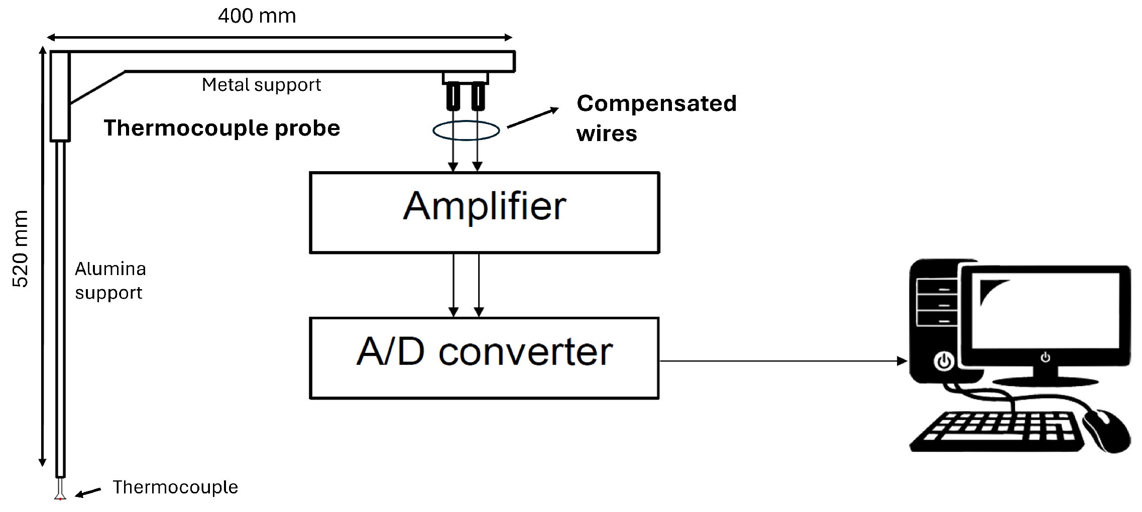
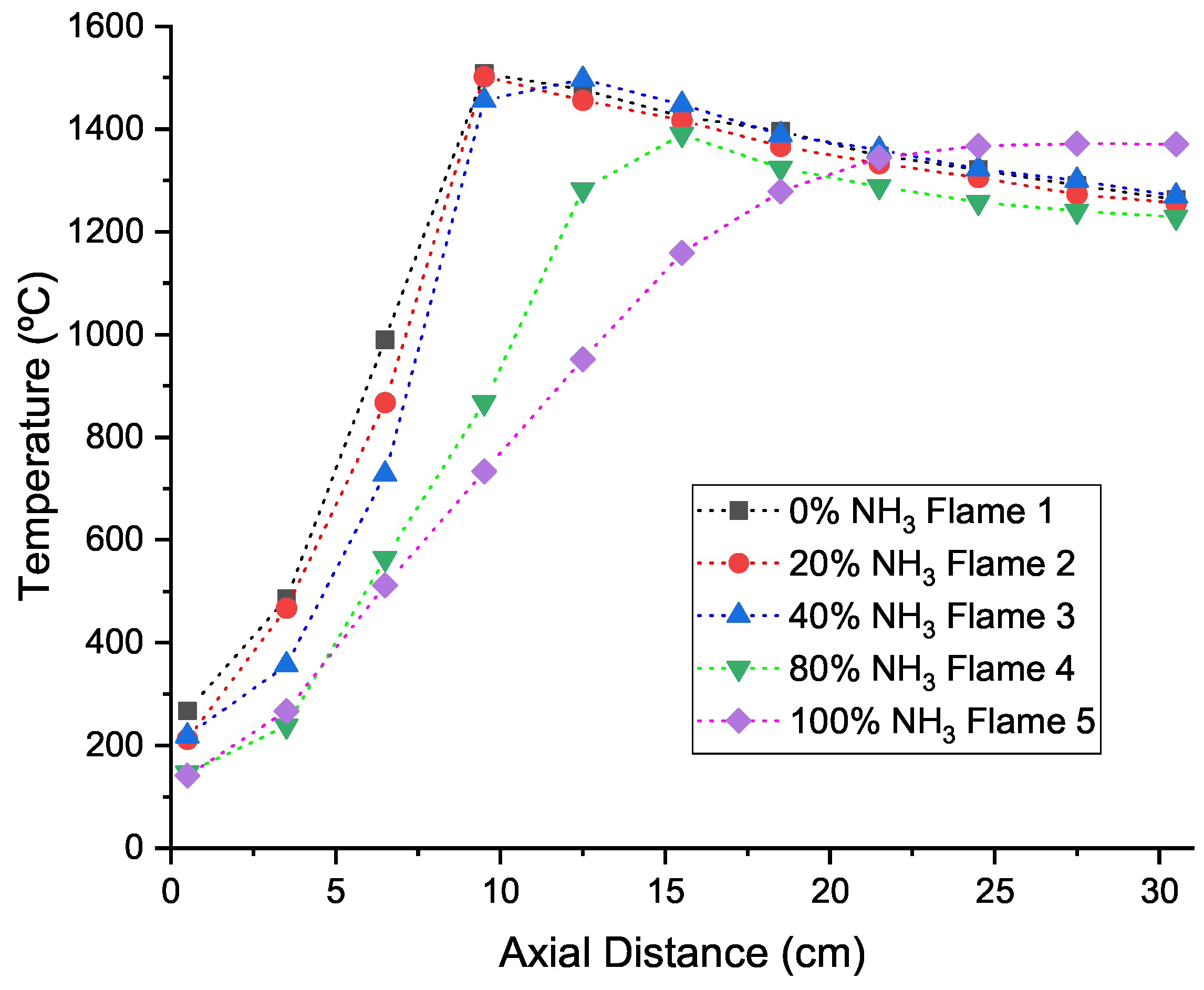
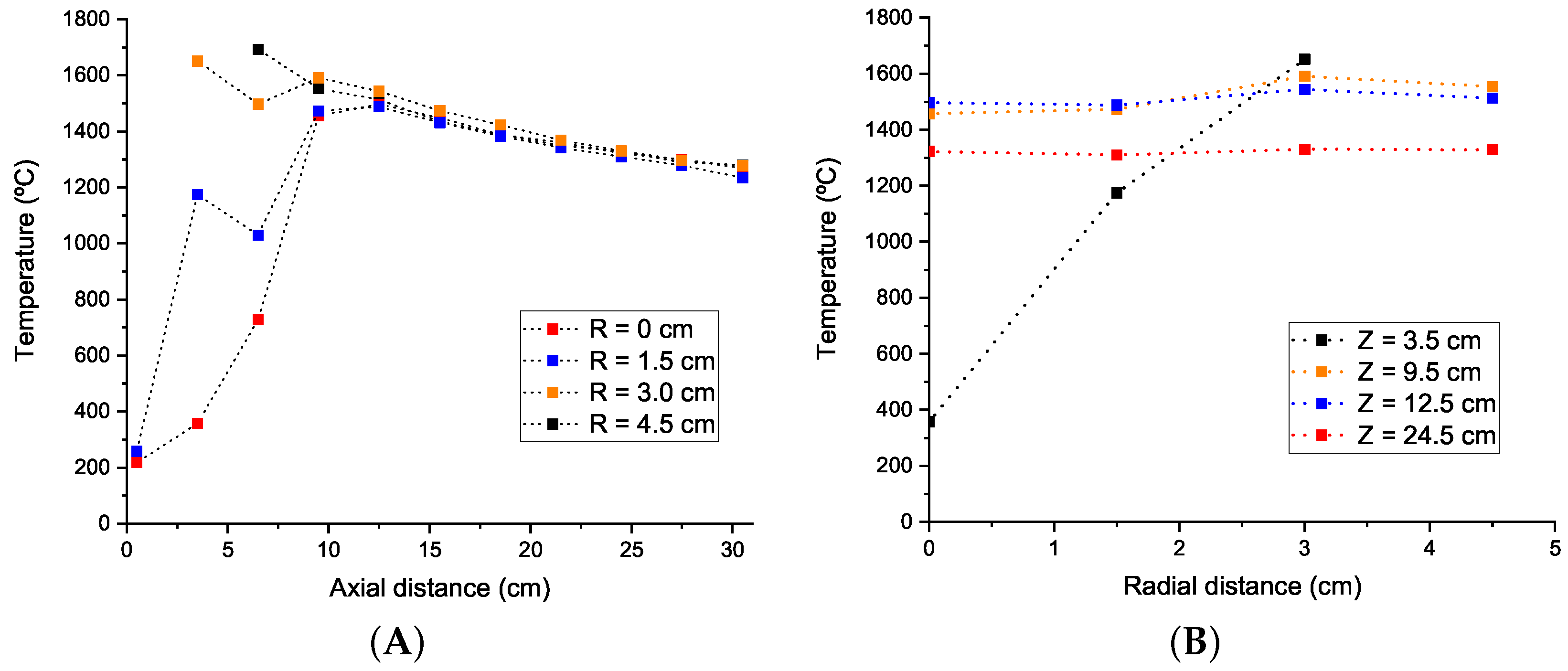
4.1. Temperature Results

In this subsection, the temperature profiles obtained for the different flames previously referred to in Table 4 will be addressed. Figure 8 shows the temperature profiles for Flame 1 measured using two different thermocouples (76 μm and 50 μm). The axial temperature profile comparison was done to assess the influence of the thermocouple diameter on the temperature measurements. Flame 1 was selected because it is where the highest temperature was expected. It can be seen that the 50 μm thermocouples recorded the highest temperature due to a reduction in radiative losses. The thermocouples exhibited deviations in their temperature measurements, with a temperature increase of 15% on average for the temperatures measured above 1000 K. This value was used as a correcting factor for the measurements in the remainder of this study. In order to obtain the correcting factor for the thermocouple, the multi-element method was used. This method consists of using multiple wires of different diameters to measure the same temperature at the same position. The error due to the radiation heat loss was estimated using an analytical expression obtained by applying the energy balance for each thermocouple bead. DE [36] presented an analytical solution using two wire and three wire methods for correcting thermocouple errors. In this study, only the two wire method was used. The analytical expressions are independent of the thermocouple material emissivity and heat transfer coefficient between the thermocouple and the flame. Hence, it is only necessary to know the wire diameters and the measured temperatures [37]. The actual gas temperature is obtained as follows:

$$T_g=T_1+{\displaystyle \frac{T_1-T_2}{\sqrt{\frac{D_2}{D_1}}\left(\frac{T_1^4-T_{ambient}^4}{T_2^4-T_{ambient}^4}\right)-1}}$$

(15)

Figure 9 shows the experimental axial temperature profiles for all the flames. It can be observed that flame 1’s peak temperature is the closest to the fuel inlet. With the increase in the NH₃ content of the fuel, the flame peak temperature moved away from the burner inlet. In the case of an NH₃ content up to 40%, the peak temperature shifts less than 3 cm relative to the peak temperature of flame 1. Even though the burner was able to operate under all conditions, significant changes in the temperature profile were noticed for flames with an NH₃ content above 40%. It can be observed that the increase in the NH₃ content leads to a less pronounced and steep temperature increase along the centerline. In the limiting case of 100% NH₃ there is no well-defined peak temperature. Additionally, it should be noted that the outlet temperature presents relatively similar values for all cases, with the exception of case 5.

Flame 3 was selected for a more detailed study to increase the knowledge of dual fuel applications and to compare against the results obtained in the numerical simulations. Figure 10 shows the temperature profiles for the burner operating at 40% NH₃ (flame 3). Figure 10A shows the axial profiles taken at different distances from the centerline, and Figure 10B shows radial profiles taken at different axial stations. It can be observed that the peak flame temperature is attained closer to the burner inlet at larger radial distances from the centerline. The flame front was stabilized in the outer region of the quarl. Downstream of Z = 9.5 cm, the temperature evolution is very similar, and the temperature is relatively homogeneous. This trend can also be observed in the radial temperature profiles presented in Figure 10B.

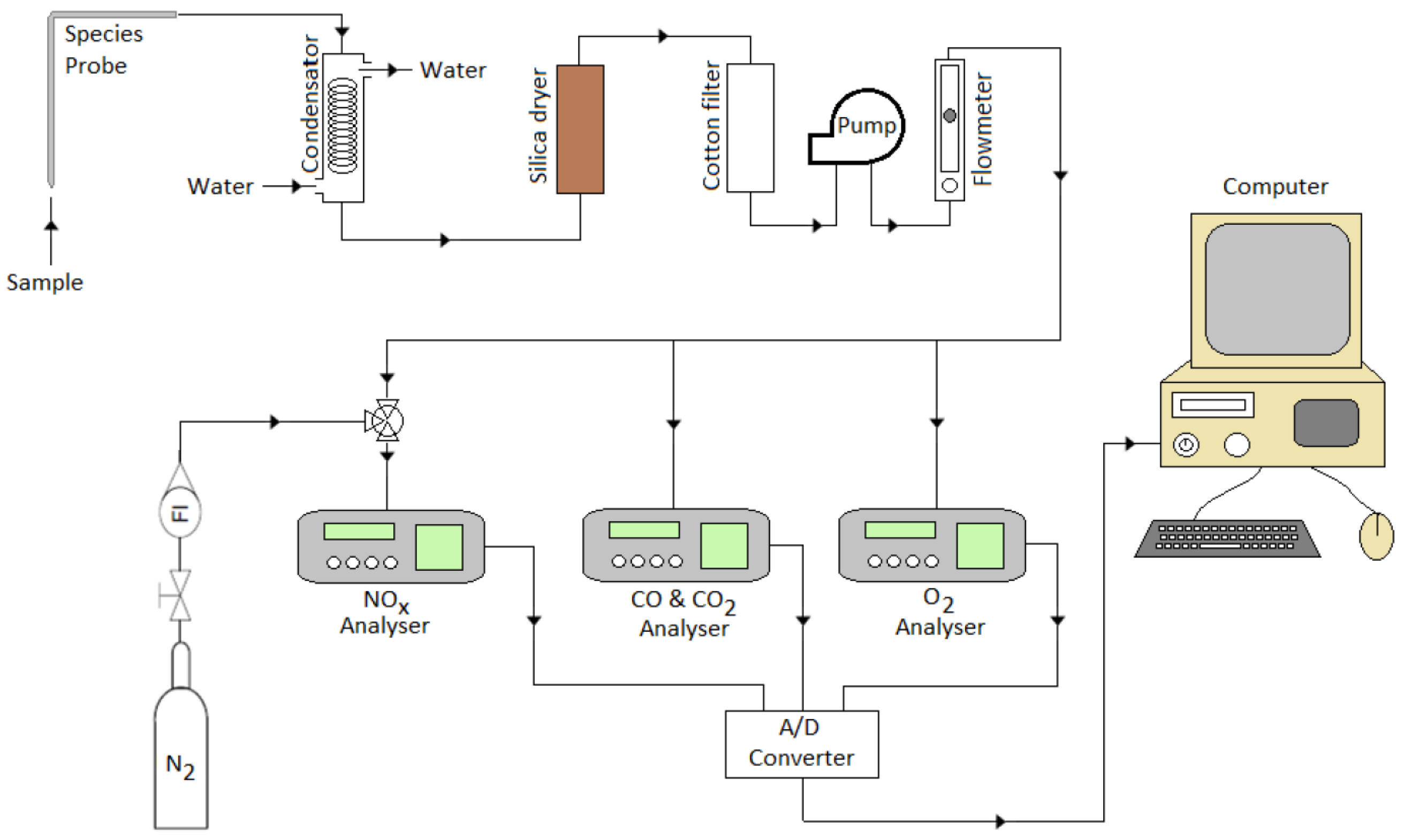
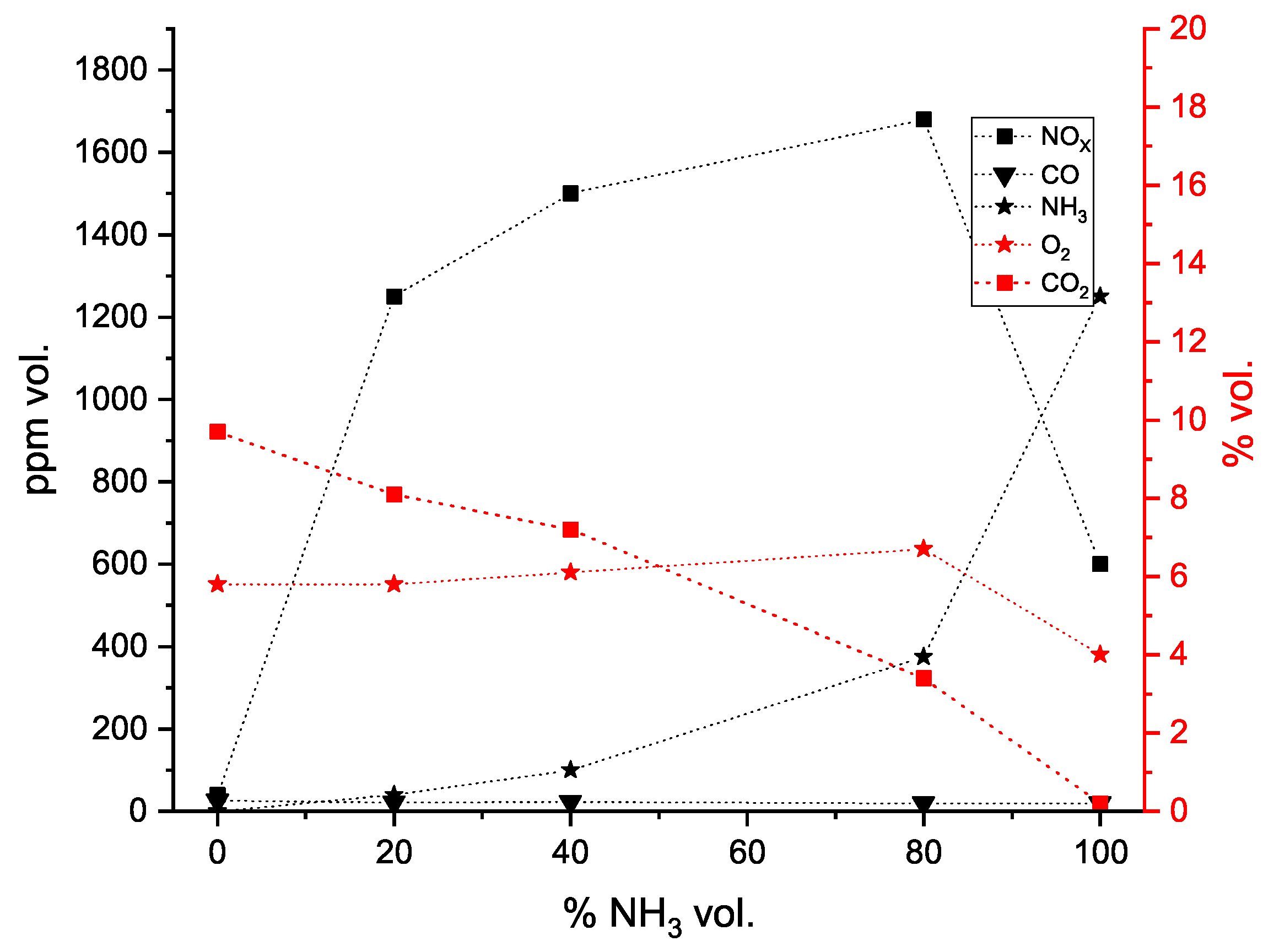
4.2. Flue Gas Emissions

The measurements of the species concentration at the exit of the combustor were obtained using two different methods, namely GASTEC tubes, measuring NO_x and NH₃, respectively, and a gas analyzer to measure NO_x, CO, CO₂, and O₂. The GASTEC tubes had very similar mean values for NO_x when compared with the gas analyzer, even though they also exhibited a higher uncertainty than the gas analyzer. Hence, in this work, only the gas analyzer was used for the NO_x measurements. Figure 11 shows the experimental dry exhaust gas emissions. Several observations can be made from these results. The emissions of CO₂ are reduced with the increase in the NH₃ content due to the reduction of fuel carbon content. However, this reduction is accompanied by increased NH₃ slip in the exhaust gas. Additionally, it can be observed that NO_x emissions increase sharply with the addition of small amounts of NH₃, e.g., the addition of just 20% NH₃ leads to 1280 ppm in exhaust gas, which is above any legislative limit. Further increase in the NH₃ content results in a corresponding increase in the NO_x emissions. The highest NO_x measurements were 1680 ppm for ${\mathrm{x}}_{N{H}_3}$ = 0.8. However, a significant reduction in the ${\mathrm{NO}}_X$ emissions is observed as ${\mathrm{x}}_{N{H}_3}$ increases from 0.8 to 1. The axial temperature profile for flame 5 exhibits significant deviations compared to other flames. Flame 5 did not display a pronounced peak in flame temperature, with the highest temperature being achieved further downstream at z = 27.5 cm. Moreover, this condition still presented a stable flame inside the combustion chamber. The addition of ammonia to the fuel mixture is accompanied by a flame temperature reduction, and NO_x emissions increase. However, when the ammonia content rises above 80%, the NO_x emissions are reduced. The NO_x emissions behavior can be observed in Figure 11. Additionally, it can also be observed the effects of NH₃ content on the axial flame temperature measurements in Figure 9. The reduction in NO_x emissions may be attributed to both the influence of lower temperatures, which mitigate NO_x formation, and incomplete combustion processes, considering the increase in ammonia slip to 1250 ppm. The ammonia slip increase is accompanied by a reduction in the NO_x emissions. This reduction in NO_x emissions is accompanied by an expected loss of efficiency since there is an increase in the unburnt fuel. Flame 5 is characterized by a smooth temperature increase with a reduced slope when compared to the other flames, and the flame front is not well defined. For natural gas, a flame front and a peak flame temperature close to the burner inlet can be observed. The natural gas flame exhibits the lowest NO_x emissions of this study, which highlights the higher efficiency of natural gas flames since most exhaust gases are complete combustion products.

The global warming potential (GWP) is an index that measures how much infrared thermal radiation a greenhouse gas will absorb over a given time frame after it has been added to the atmosphere (or emitted by the atmosphere). The GWP allows for the comparison between different greenhouse gases regarding their “effectiveness in causing radiative forcing” [38]. The GWP index can be used to estimate the impact caused by the introduction of ammonia and other alternative fuels in the mitigation of greenhouse gas emissions. Figure 12 shows the theoretical maximum GWP reduction achieved via direct NH₃ combustion, referred to as ${\mathrm{GWP}}_{Dual-fuel}$. The theoretical maximum GWP reduction only takes into account the decrease in CO₂ emissions.The emissions of N₂O are not shown due to the absence of the means to measure them experimentally. However, the figure shows the maximum allowable N₂O emissions to maintain a GWP ≤ 1 (lower than conventional natural gas emissions); if N₂O emissions are maintained below these directive values, blends of NH₃ in natural gas can be implemented to reduce the greenhouse warming potential in comparison to natural gas (100% CH₄) combustion applications over a reduced timeframe. It should be noted that N₂O is a greenhouse gas 273 times more powerful than CO₂ in a 100-year timeframe, so even a small amount of N₂O can increase the GWP [39].

Previous works have studied the production of N₂O under lean conditions. The authors [40] stated that N₂O production increases sharply for NH₃/H₂ blends with more than an 80% NH₃ content. This again can be attributed to increased heat losses and the decreased presence of H₂ in the flame that lead to an incomplete combustion process, which reduces H radical production, thereby restricting N₂O consumption through the reaction N₂O + H ⇌ N₂ + OH. NO and NO₂ emissions decreased with the increasing ammonia content in the fuel. However, N₂O emissions followed the opposite trend as NO is consumed along with NH to produce N₂O. Increased N₂O emissions in flames with a high concentration of ammonia (${\mathrm{x}}_{{\mathrm{NH}}_3}$≥ 0.8) were attributed to increased heat losses and greater production of NH radicals [40]. In this study, concentrations of N₂O were under 50 ppm for ${\mathrm{x}}_{{\mathrm{NH}}_3}$≤ 0.8, aligning with a reduction in GWP compared to the methane GWP. The author’s conclusions are consistent with the observations in the present study where for ${\mathrm{x}}_{{\mathrm{NH}}_3}$≥ 0.8, a reduction in NO_x emissions and an increase in the ammonia slip are observed, hinting at an incomplete oxidation process that may lead to the production of N₂O. Okafor et al. [7] also performed experimental tests where a single-stage combustor produced 580 ppm of N₂O and a two-stage rich–lean combustor where N₂O concentrations were below 80 ppm at 16% O₂, highlighting the potential of different combustion strategies for reducing N₂O emissions. Overall, it was concluded that lean ammonia/hydrogen combustion under industrially representative equivalence ratios might lead to the possibility of high N₂O emissions for high ammonia contents, limiting the applicability of the concept and potentially the direct, minor retrofitting of current gas turbines to employ fuels with a high ammonia content.

5. Numerical Results

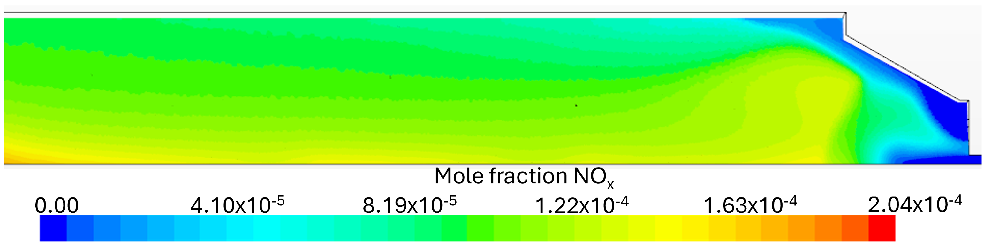
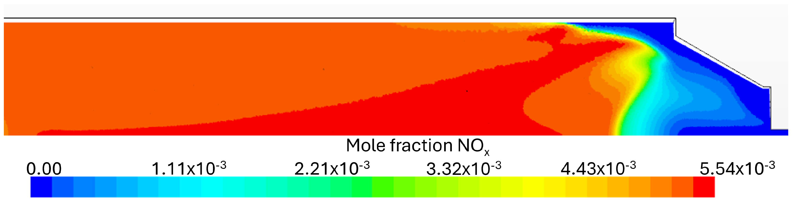
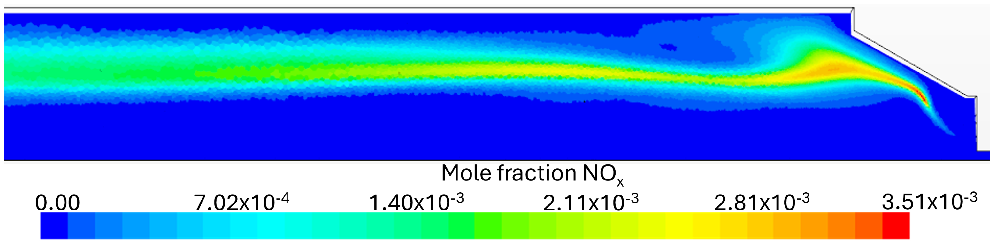
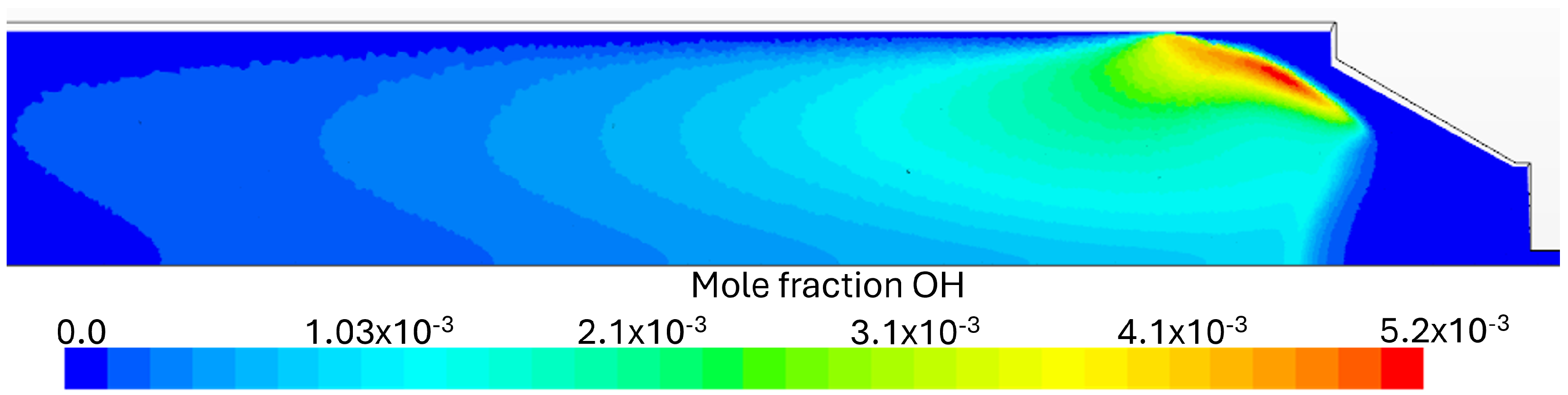
The results obtained from the numerical simulations are presented and discussed in this section, and the experimental data are used for validation. The boundary conditions presented in

Table 5. Boundary conditions.

Boundary	Momentum Equation	Energy Equation
Inlet-fuel	mass flow = $1.404\times {10}^{-5}$ kg/s	$T=300\mathrm{K}$
Inlet-air	mass flow = $1.726\times {10}^{-4}$ kg/s	$T=300\mathrm{K}$
Outlet	Pressure Outlet	$T=300\mathrm{K}$
Wall		$T_{\mathrm{wall}}=1000\mathrm{K}$

were implemented to simulate flame 3 (see Table 4).

Previous computational studies revealed a slip angle of less than 1° from the co-flow air inlet to the vane angle [41]. The co-flow angle refers to the angle at which the flow is directed parallel to the rotational axis of the burner. It was found that for these conditions, it can be assumed that the vane angle is equal to the inlet flow angle. Hence, the assumed co-flow angle for the air inlet was 45°. Based on measurements obtained using a type-K thermocouple, the wall temperature of the combustion chamber ranges from 972 K to 1043 K. This temperature range reflects the thermal conditions present for the combustion chamber wall during operation. Consequently, a wall temperature of 1000 K was selected for the boundary conditions. Simulations with lower wall temperatures (900 K and 800 k) were performed, and the results presented lower exhaust temperatures, and their peak flame temperature did not suffer a significant impact.

Figure 13, Figure 14 and Figure 15 show the temperature contours inside the combustion chamber for flames 1, 3, and 5. The peak temperature in the combustion chamber is located downstream of the quarl exit in its outer region for the flames containing natural gas in their fuel composition. Flame 1 had the highest flame temperature with a peak of 1792 °C. The addition of 40% NH₃ into the fuel mixture led to a small reduction in the peak flame temperature to 1766 °C, and the peak temperature location did not suffer a significant shift in its position. Flame 5 exhibited a very distinct temperature contour, the flame was not stabilized at the quarl exit and exhibited the lowest peak flame temperature out of all the simulations. The flame has a very elongated shape, which is in accord with the experimental results.

Figure 16, Figure 17 and Figure 18 display the axial velocity and the flow pattern across the simulation domain. A recirculation zone is observed at the quarl exit for all the simulated conditions. The addition of ammonia in the fuel mixture leads to an increase in the inlet velocity that impacts the recirculation in the combustion chamber. This phenomenon was more noticeable in simulations with more than 40% ammonia in the fuel mixture, where it generated a flowfield with a higher fuel inlet penetration and an outward shift in the recirculation zone. The observed trends highlight the influence of different fuel properties during flexible fuel operation, which have a significant impact on the flow field, temperature field, and exhaust emissions.

Figure 19 shows a comparison between the numerical and experimental axial temperature profiles and a comparison between the numerical and experimental results for flames 1, 3, and 5. Numerical simulations for flames with CH₄ in their fuel mixture overpredicted the peak flame temperature compared with the experimental results. Simulations for flame 5 predicted lower peak temperatures than the experimental results. However, it should be noted simulations were able to reproduce the temperature profile up to z = 12.5 cm; from this point onwards, simulations presented a deviation from the experimental results. The model was able to qualitatively capture the effect of the ammonia content in the fuel mixture on the axial temperature profiles.

Figure 20 shows a comparison between the numerical and experimental axial temperature profiles at different distances from the centerline for flame 3. For the evaluation of the temperature profile, Z represents the distance from the burner inlet along the burner center line and R represents the distance from the centerline.

It can be observed that the simulations qualitatively capture the axial temperature profile’s behavior in the burner. For flame 3, the simulation predicted a peak temperature of 1549 °C at Z = 7.9 cm, while the experimental results showed a peak of 1512 °C at Z = 12.5 cm. Additionally, for the two most central positions, Figure 20a,b, the numerical simulations overpredicted both the peak temperature and its location, which is predicted to be closer to the burner inlet, even though the simulations were able to qualitatively reproduce the measured temperature profile. The outer profiles in Figure 20c,d exhibited the opposite behavior, with the experimental profiles exhibiting a peak flame temperature closer to the burner inlet, with a measured maximum gas temperature of 1693 °C. The evolution of the temperature profiles downstream of Z = 12.5 cm is in better agreement with the experimental data apart from a slightly larger deviation for R = 4.5 cm Figure 20d. Figure 21 show the comparison between the numerical and experimental radial temperature profiles. The numerical prediction closely matches the experimental data except for Z = 3.5 cm, where the simulations exhibited a large deviation near the combustion chamber walls.

The model using complex chemistry was able to predict rather satisfactorily the axial temperature profiles despite overpredicting the peak flame temperatures and underpredicting the near-wall temperatures in the quarl zone. The temperature offset might arise from the underprediction of heat transfer at the combustor inlet and quarl walls since the temperature and emissivity of the walls were guesses. Future experimental works should detail the heat loss from the burner tip and its support structure.

Flue Gas Emissions

In this section, the emissions obtained from the simulations and experimental results are compared. For this type of analysis, the chemistry kinetics and combustion model greatly influence the results. Simpler combustion models overpredict fuel conversion in the combustor, which leads to the assumption of complete combustion and a nonreliable analysis of the flue gas components. On the other hand, complex chemistry models capture intermediary reactions and the production of pollutants (NO_x) or incomplete combustion that is manifested as ammonia slip. Figure 22 shows a comparison between the measured flue gas emissions and the values predicted by the simulation for flames 1, 3, and 5. The numerical predictions of the flue gas composition were obtained by calculating the average species concentration over a cross-sectional area of the computational domain, aligned with the burner exit and corresponding to the position of the gas analysis probe. Despite being positioned along the centerline, the acquired sample reflects the averaged composition of the probe’s local surroundings.

For simulations with natural gas in the flame’s fuel mixture, the model achieved complete combustion with zero fuel concentration in the exhaust. Flame 3 greatly overpredicted the NO_x emissions, yielding 6065 ppm of NO_x compared with the experimental results of 1500 ppm. This discrepancy can be attributed mainly to two different factors. First, the kinetic mechanism might overestimate the NO_x production, as reported in previous works [40]; Second, the numerical simulations predict higher temperatures in the flowfield, leading to a higher NO_x concentration in the simulations results. This increase in the NO_x can be attributed to the thermal NO_x formation pathway in the inner recirculation zone where the reactions N + OH ⇌ NO + H, N + O₂⇌ O + NO and N₂ + O ⇌ NO + N play the most significant role in the production of NO [42]. For flame 5, the model was able to qualitatively predict the NO_x emission trend and presented a value in agreement with the experimental results. Moreover, the model predicted CO₂ and CO emissions that are in agreement with the experimental results. Figure 23, Figure 24 and Figure 25 show the mole fraction contours of NO_x, Figure 26, Figure 27 and Figure 28 show the mole fraction contours of OH, and Figure 29, Figure 30 and Figure 31 show the mole fraction contours of N₂O for the three simulated conditions. Substantial levels of OH radicals are generated in the peak flame temperature region in all the simulations. The subsequent consumption of OH radicals by the flames with ammonia contributes significantly to the formation of NO. Flame 3 predicted no N₂O emissions even though it predicts its formation and subsequent destruction, which can be attributed to the presence of high temperatures and a high concentration of OH radicals, leading to the complete consumption of N₂O through the reaction pathway N₂O + H ⇌ N₂ + OH. Flame 5 predicted much higher N₂O emissions (215 ppm vol.), the reduction in OH mole fraction and narrow distribution on the flowfield indicates the presence of incomplete combustion, hence incomplete oxidation of the NH₃ and high production of N₂O. This behavior is consistent with the previous literature findings, where N₂O and NO emissions followed the opposite trend [40].

Ammonia combustion is known for its high NO emissions when burning under lean conditions. Previous experimental works on ammonia combustion have already reported NO emissions in the range between 2000 and 5000 ppm, which is similar to range in the simulation results [35]. In order to produce more accurate results for emissions, the heat transfer process must be addressed in more detail since it greatly influences the NO and N₂O formation process [40]. A more accurate temperature field will likely produce more accurate NO_x predictions and NH₃ slip in flue gas emissions. The kinetic mechanism predicts the complete oxidation of the ammonia content in the combustion chamber. This only occurs for simulations with relatively high CH₄ content, namely flames 1 and 3. Moreover, it should be noted that the experimental results yielded a concentration of only 100 ppm, and the absolute deviations from the experimental results are relatively small for this condition. For flame 5, the opposite behavior is observed. For these conditions, numerical simulations yielded a very large deviation from the experimental results with respective emissions of 23,078 ppm vol. and 1250 ppm vol. Simulations greatly overpredicted the amount of unburnt ammonia and predicted the appearance of incomplete combustion for flame 5. The phenomenon can be attributed to the high concentration of OH radicals associated with the CH₄ combustion process that would promote complete oxidation of the fuel. For mixtures with a low content of CH₄ in the fuel mixture, the production of OH is reduced, as can be observed in Figure 27 and Figure 28, leading to an incomplete combustion process. It should be noted that experimental results might underpredict NH₃ slip due to the dilution and reaction of NH₃ in the water condensation of the drying system before entering the gas analyzer.

The simulations predicted very similar results compared to the theoretical results for the emissions of CO₂. Predictions for the CO₂ only presented a deviation of 0.2% in terms of dry volume fraction.

The NO_x and NH₃ emissions from flames with ammonia added to their mixture are not compliant with current legislative limits. Possible solutions to mitigate NO_x emissions might include the integration of post-combustion treatments such as SCR (selective catalytic reduction) in order to address the exhaust gas from the actual ammonia combustion contaminants such as unburned ammonia, nitrogen oxides (NO_x), and nitrous oxide (N₂O). Unburned ammonia can be removed by using a conventional oxidation catalyst, but NO_x and N₂O are simultaneously generated as byproducts. Therefore, new catalysts that can remove ammonia with high efficiency while reducing the generation of NO_x and N₂O are necessary for implementing ammonia combustion as an alternative energy source. The drawback of the SCR catalyst is that it requires the injection of ammonia as a reducing agent, which would increase the ammonia consumption and reduce the overall energy efficiency. Other solutions that might help in the mitigation of pollutants and increase combustion efficiency might be the implementation of alternative combustion strategies, such as staged combustion or mild combustion.

6. Conclusions

In this work, it was possible to stably operate a swirl burner in a dual-fuel configuration with ammonia concentrations ranging from 0% to 100% by volume in the fuel mixture. This study evaluates combustion performance, specifically flame stability, as well as the influence of NH₃ content in a combustor powered by a swirl diffusion burner. The developed combustor can be fired using blends of natural gas and NH₃ without the risk of blow-off while maintaining a stable and attached flame. Additionally, numerical simulations were performed to aid in the design and implementation of ammonia combustion. The main goal is to explore a cost-effective model for predicting the flames resulting from natural gas/NH₃ combustion. The principal conclusions drawn from this analysis can be summarized as follows:

• Regarding the industrial application, there are several relevant implications that can be drawn from this study. First, it was experimentally demonstrated that a conventional gas burner, typically used in the industry, can operate stably using pure NG and its blends with up to 100% vol. of NH₃. It was verified that the flame stability was maintained with the addition of NH₃. This implies that, in an industrial context, fuel-flexible burners have the readiness and potential to serve as a cost-effective and efficient transitional technology for blending NH₃ with conventional fossil fuels as a strategy to offset the carbon emissions of combustion systems in the near future.
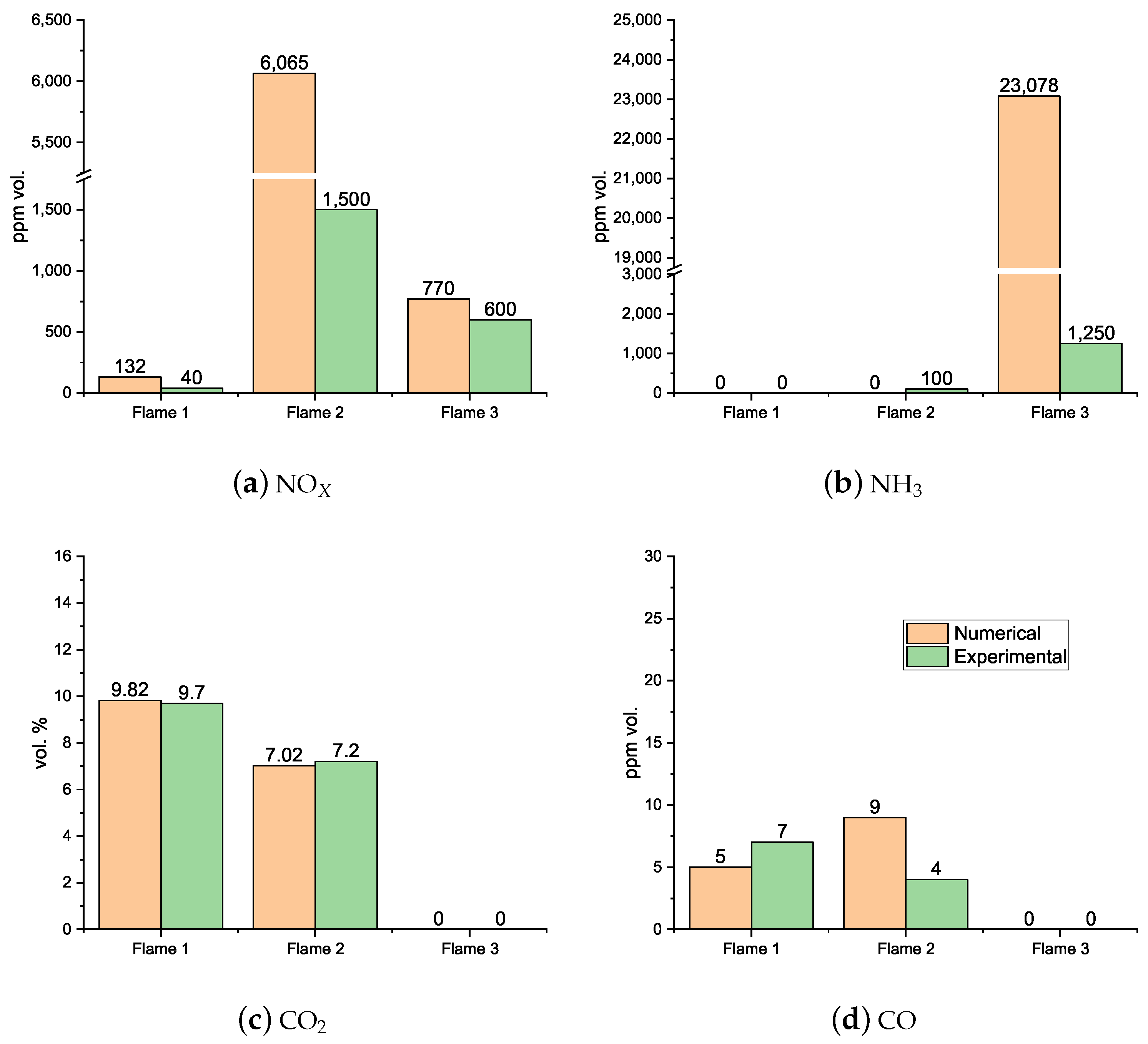
• It was observed that even with the burner firing small amounts of NH₃, there were still high NO_x emissions, highlighting the necessity for post-combustion flue gas treatment, namely SCR (selective catalytic reduction) or staged combustion applications such as RQL (Rich–quench–Lean) for industrial applications. At higher fuel NH₃ content, a substantial ammonia slip was detected in the exhaust gas emissions at 80% NH₃. The presence of unburned NH₃ and the formation of N₂O are limiting factors in ammonia combustion applications due to their toxicity and GWP (greenhouse warming potential), respectively.
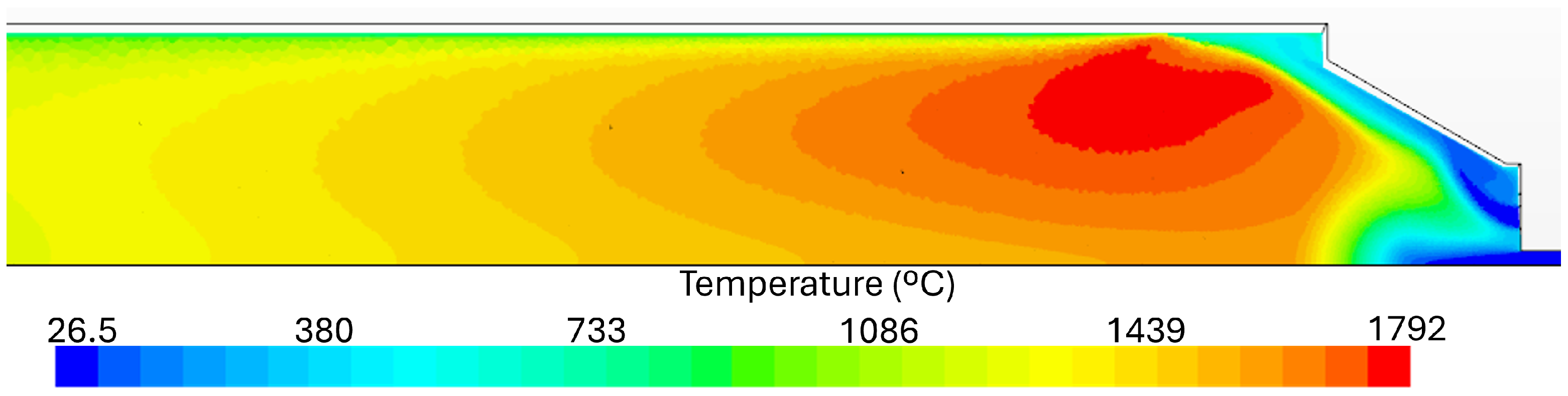
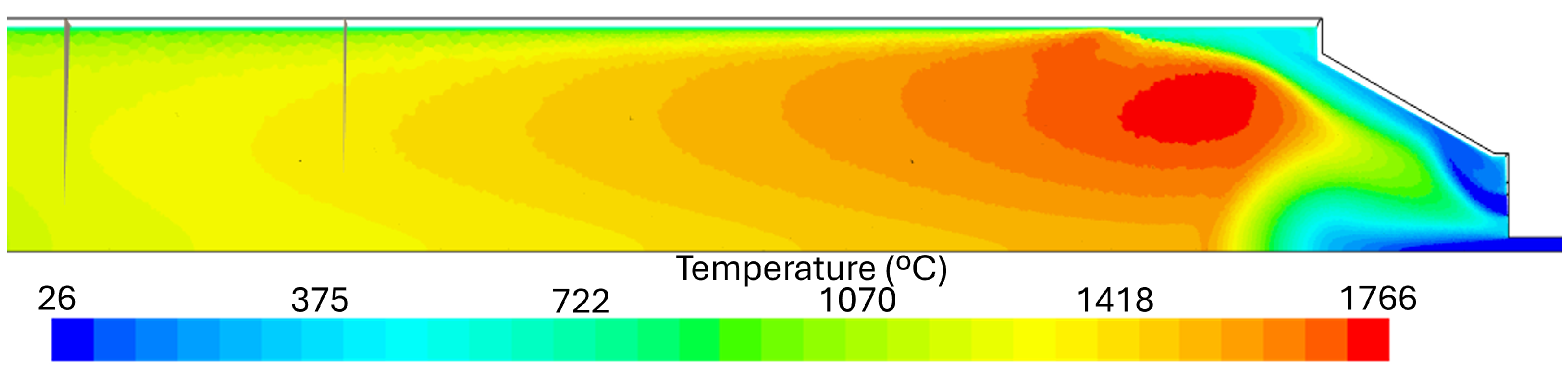
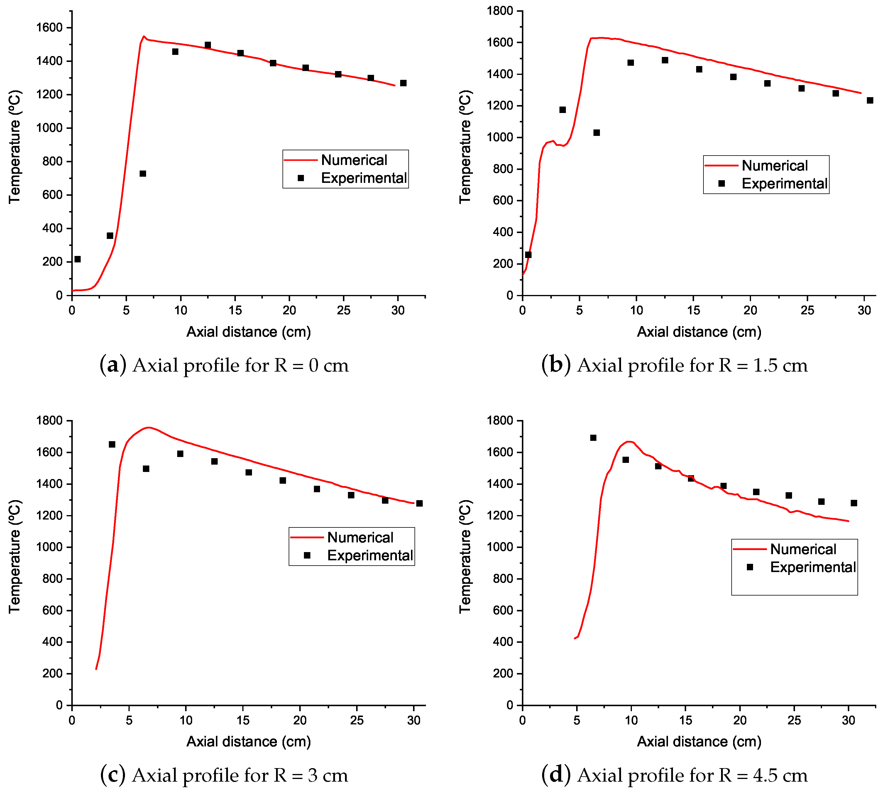
• Numerical simulations were able to qualitatively predict the axial temperature profiles of the experimental burner even though simulations with natural gas in their fuel mixture overpredicted the peak flame temperature. Downstream of this peak, the numerical simulations accurately predict the temperature profile up to the burner exit.
• It can be concluded that a cost-effective simulation can be used to qualitatively predict the experimental combustor’s flame characteristics. Complex chemistry models and detailed kinetic mechanisms were necessary to model the ammonia/natural gas multicomponent combustion process. However, simulations were not able to capture the NO_x and NH₃ emissions for some conditions, namely for flame 3 (40% NH₃) and the NH₃ slip emissions for flame 5 (100% NH₃).

References

1. Commission Regulation (EU) No 813/2013. 2013. Available online: https://eur-lex.europa.eu/eli/reg/2013/813/2017-01-09 (accessed on 1 April 2024).
2. Valera-Medina, A.; Syred, N.; Griffiths, A. Visualisation of isothermal large coherent structures in a swirl burner. Combust. Flame 2009, 156, 1723–1734. [Google Scholar] [CrossRef]
3. Yapicioglu, A.; Dincer, I. Performance assesment of hydrogen and ammonia combustion with various fuels for power generators. Int. J. Hydrogen Energy 2018, 43, 21037–21048. [Google Scholar] [CrossRef]
4. American Chemical Society. Ammonia. Available online: https://www.acs.org/molecule-of-the-week/archive/a/ammonia.html (accessed on 15 February 2024).
5. da Rocha, R.C.; Costa, M.; Bai, X.S. Chemical kinetic modelling of ammonia/hydrogen/air ignition, premixed flame propagation and NO emission. Fuel 2019, 246, 24–33. [Google Scholar] [CrossRef]
6. Møller, M.M.K. Managing Emissions from Ammonia-Fueled Vessels. Center for Zero Carbon Shipping (MMMCZCS). Available online: https://cms.zerocarbonshipping.com/media/uploads/documents/Ammonia-emissions-reduction-position-paper_v4.pdf (accessed on 10 May 2024).
7. Okafor, E.C.; Tsukamoto, M.; Hayakawa, A.; Somarathne, K.A.; Kudo, T.; Tsujimura, T.; Kobayashi, H. Influence of wall heat loss on the emission characteristics of premixed ammonia-air swirling flames interacting with the combustor wall. Proc. Combust. Inst. 2021, 38, 5139–5146. [Google Scholar] [CrossRef]
8. Pugh, D.; Bowen, P.; Valera-Medina, A.; Giles, A.; Runyon, J.; Marsh, R. Influence of steam addition and elevated ambient conditions on NOx reduction in a staged premixed swirling NH3/H2 flame. Proc. Combust. Inst. 2019, 37, 5401–5409. [Google Scholar] [CrossRef]
9. Okafor, E.C.; Somarathne, K.A.; Ratthanan, R.; Hayakawa, A.; Kudo, T.; Kurata, O.; Iki, N.; Tsujimura, T.; Furutani, H.; Kobayashi, H. Control of NOx and other emissions in micro gas turbine combustors fuelled with mixtures of methane and ammonia. Combust. Flame 2020, 211, 406–416. [Google Scholar] [CrossRef]
10. Manna, M.V.; Sabia, P.; Raffaele, R.; Mara, d.J. NH3 effect on CH4 oxidation regimes and chemical kinetics. In Proceedings of the European Combustion Meeting, Rouen, France, 26–28 April 2023; pp. 760–765. [Google Scholar]
11. Cheng, J.; Zhang, B. Analysis of explosion and laminar combustion characteristics of premixed ammonia-air/oxygen mixtures. Fuel 2023, 351, 128860. [Google Scholar] [CrossRef]
12. Cheng, J.; Zhang, B. Experimental study on the explosion characteristics of ammonia-hydrogen-air mixtures. Fuel 2024, 363, 131046. [Google Scholar] [CrossRef]
13. Sun, J.; Yang, Q.; Zhao, N.; Chen, M.; Zheng, H. Numerically study of CH4/NH3 combustion characteristics in an industrial gas turbine combustor based on a reduced mechanism. Fuel 2022, 327, 124897. [Google Scholar] [CrossRef]
14. Mashruk, S.; Vigueras-Zuniga, M.; del Cueto, M.T.; Xiao, H.; Yu, C.; Maas, U.; Valera-Medina, A. Combustion features of CH4/NH3/H2 ternary blends. Int. J. Hydrogen Energy 2022, 47, 30315–30327. [Google Scholar] [CrossRef]
15. Shih, T.H.; Liou, W.W.; Shabbir, A.; Yang, Z.; Zhu, J. A New k-ϵ Eddy Viscosity Model for High Reynolds Number Turbulent Flows—Model Development and Validation. Comput. Fluids 1995, 24, 227–238. [Google Scholar] [CrossRef]
16. Spalart, P.R.; Rumsey, C.L. Effective Inflow Conditions for Turbulence Models in Aerodynamic Calculations. AIAA J. 2007, 45, 2544–2553. [Google Scholar] [CrossRef]
17. Siemens Industries Digital Software Realizable K-epsilon model. In SIEMENS STAR-CCM+ Documentation; Siemens: Munich, Germany, 2020.
18. Okafor, E.C.; Naito, Y.; Colson, S.; Ichikawa, A.; Kudo, T.; Hayakawa, A.; Kobayashi, H. Experimental and numerical study of the laminar burning velocity of CH4–NH3–air premixed flames. Combust. Flame 2018, 187, 185–198. [Google Scholar] [CrossRef]
19. Smith, G.P.; Golden, D.M.; Frenklach, M.; Moriarty, N.W.; Eiteneer, B.; Goldenberg, M.; Bowman, C.T.; Hanson, R.K.; Song, S.; Gardiner, W.C., Jr.; et al. Available online: http://www.me.berkeley.edu/gri_mech/ (accessed on 5 August 2024).
20. Tian, Z.; Li, Y.; Zhang, L.; Glarborg, P.; Qi, F. An experimental and kinetic modeling study of premixed NH3/CH4/O2/Ar flames at low pressure. Combust. Flame 2009, 156, 1413–1426. [Google Scholar] [CrossRef]
21. Siemens Industries Digital Software Participating Media Radiation (DOM). In SIEMENS STAR-CCM+ Documentation; Siemens: Munich, Germany, 2020.
22. Modest, M. Narrow-band and full-spectrum k-distributions for radiative heat transfer—Correlated-k vs. scaling approximation. J. Quant. Spectrosc. Radiat. Transf. 2003, 76, 69–83. [Google Scholar] [CrossRef]
23. Tarek Echekki, E.M. (Ed.) Turbulent Combustion Modeling; Springer: Dordrecht, The Netherlands, 2013. [Google Scholar]
24. Siemens Industries Digital Software Reacting Species Transport. In SIEMENS STAR-CCM+ Documentation; Siemens: Munich, Germany, 2020.
25. Stiehl, B.; Worbington, T.; Miegel, A.; Martin, S.; Velez, C.; Ahmed, K. Combustion and Emission Characteristics of a Lean Axial-Stage Combustor. In Proceedings of the ASME Turbo Expo 2019: Turbomachinery Technical Conference and Exposition, Phoenix, AZ, USA, 17–21 June 2019. Volume 4B: Combustion, Fuels, and Emissions, Turbo Expo: Power for Land, Sea, and Air. [Google Scholar] [CrossRef]
26. Stiehl, B.; Genova, T.; Otero, M.; Reyes, J.; Ahmed, K.A.; Martin, S.M. NOx Emission of an Axial-Staged Combustor at High-Pressure. In Proceedings of the AIAA Propulsion and Energy 2020 Forum, Virtual, 24–28 August 2020. [Google Scholar] [CrossRef]
27. Bösenhofer, M.; Wartha, E.M.; Jordan, C.; Harasek, M. The Eddy Dissipation Concept—Analysis of Different Fine Structure Treatments for Classical Combustion. Energies 2018, 11, 1902. [Google Scholar] [CrossRef]
28. Halouane, Y.; Dehbi, A. CFD simulations of premixed hydrogen combustion using the Eddy Dissipation and the Turbulent Flame Closure models. Int. J. Hydrogen Energy 2017, 42, 21990–22004. [Google Scholar] [CrossRef]
29. Mousavi, S.M.; Sotoudeh, F.; Jun, D.; Lee, B.J.; Esfahani, J.A.; Karimi, N. On the effects of NH3 addition to a reacting mixture of H2/CH4 under MILD combustion regime: Numerical modeling with a modified EDC combustion model. Fuel 2022, 326, 125096. [Google Scholar] [CrossRef]
30. Mansouri, Z.; Boushaki, T. Experimental and numerical investigation of turbulent isothermal and reacting flows in a non-premixed swirl burner. Int. J. Heat Fluid Flow 2018, 72, 200–213. [Google Scholar] [CrossRef]
31. Lorena, M. Fuel-Flexible Hydrogen Burner for Industrial Furnace Systems; Instituto Superior Técnico: Lisboa, Portugal, 2023. [Google Scholar]
32. Pacheco, G.P.; Rocha, R.C.; Franco, M.C.; Mendes, M.A.A.; Fernandes, E.C.; Coelho, P.J.; Bai, X.S. Experimental and Kinetic Investigation of Stoichiometric to Rich NH3/H2/Air Flames in a Swirl and Bluff-Body Stabilized Burner. Energy Fuels 2021, 35, 7201–7216. [Google Scholar] [CrossRef]
33. Franco, M.C.; Rocha, R.C.; Costa, M.; Yehia, M. Characteristics of NH3/H2/air flames in a combustor fired by a swirl and bluff-body stabilized burner. Proc. Combust. Inst. 2021, 38, 5129–5138. [Google Scholar] [CrossRef]
34. Ramos, C.F.; Rocha, R.C.; Oliveira, P.M.; Costa, M.; Bai, X.S. Experimental and kinetic modelling investigation on NO, CO and NH3 emissions from NH3/CH4/air premixed flames. Fuel 2019, 254, 115693. [Google Scholar] [CrossRef]
35. Rocha, R.C.; Ramos, C.F.; Costa, M.; Bai, X.S. Combustion of NH3/CH4/Air and NH3/H2/Air Mixtures in a Porous Burner: Experiments and Kinetic Modeling. Energy Fuels 2019, 33, 12767–12780. [Google Scholar] [CrossRef]
36. De, D. Measurement of flame temperature with a multielement thermocouple. J. Inst. Energy (UK) 1981, 54, 113–116. [Google Scholar]
37. Hindasageri, V.; Vedula, R.P.; Prabhu, S.V. Thermocouple error correction for measuring the flame temperature with determination of emissivity and heat transfer coefficient. Rev. Sci. Instrum. 2013, 84, 024902. [Google Scholar] [CrossRef]
38. IPCC. Annex V11: Glossary; IPCC: Geneva, Switzerland, 2021. [Google Scholar]
39. Al-Abdeli, Y.M.; Masri, A.R. Recirculation and flowfield regimes of unconfined non-reacting swirling flows. Exp. Therm. Fluid Sci. 2003, 27, 655–665. [Google Scholar] [CrossRef]
40. Mashruk, S.; Okafor, E.; Kovaleva, M.; Alnasif, A.; Pugh, D.; Hayakawa, A.; Valera-Medina, A. Evolution of N2O production at lean combustion condition in NH3/H2/air premixed swirling flames. Combust. Flame 2022, 244, 112299. [Google Scholar] [CrossRef]
41. Barreto, T.A. Numerical Validation of an Open Flame, Swirl-Stabilized, Pure Hydrogen Burner; Instituto Superior Técnico: Lisbon, Portugal, 2023. [Google Scholar]
42. Zhang, M.; An, Z.; Wei, X.; Wang, J.; Huang, Z.; Tan, H. Emission analysis of the CH4/NH3/air co-firing fuels in a model combustor. Fuel 2021, 291, 120135. [Google Scholar] [CrossRef]
Figure 1. Green ammonia production and utilization roadmap.
Energies 17 04206 g001
Figure 2. 3D periodic combustor mesh, with the highlighted refinement zones, (A) average cell size of 1 mm, (B) average cell size of 0.5 mm.
Energies 17 04206 g002
Figure 3. Mesh independency analysis.
Energies 17 04206 g003
Figure 4. Schematic of the experimental setup.
Energies 17 04206 g004
Figure 5. Burner longitudinal cross-section.
Energies 17 04206 g005
Figure 6. Schematic of the gas sampling system.
Energies 17 04206 g006
Figure 7. Schematic of the temperature measuring system.
Energies 17 04206 g007
Figure 8. Axial temperature profile comparisons for different thermocouple bead sizes.
Energies 17 04206 g008
Figure 9. Axial temperature profiles for the tested cases.
Energies 17 04206 g009
Figure 10. Axial temperature profiles at different distances from the centerline (A) and radial temperature profiles (B) for flame 3 (40% NH3 vol.).
Energies 17 04206 g010
Figure 11. Experimental exhaust gas analysis emissions, on a dry basis.
Energies 17 04206 g011
Figure 12. Comparison of greenhouse warming potential for a 100-year timeframe.
Energies 17 04206 g012
Figure 13. Temperature contours across the burner for flame 1 (0% NH3 vol.).
Energies 17 04206 g013
Figure 14. Temperature contours across the burner for flame 3 (40% NH3 vol.).
Energies 17 04206 g014
Figure 15. Temperature contours across the burner for flame 5 (100% NH3 vol.).
Energies 17 04206 g015
Figure 16. Flow pattern across the burner for flame 1 (0% NH3 vol.).
Energies 17 04206 g016
Figure 17. Flow pattern across the burner for flame 3 (40% NH3 vol.).
Energies 17 04206 g017
Figure 18. Flow pattern across the burner for flame 5 (100% NH3 vol.).
Energies 17 04206 g018
Figure 19. Comparison between numeric and experimental axial temperature profiles for flame 1 (0% NH3 vol.), flame 3 (40% NH3 vol.) and Flame 5 (100% NH3 vol.).
Energies 17 04206 g019
Figure 20. Comparison between numeric and experimental axial temperature profiles for flame 3 (40% NH3 vol.).
Energies 17 04206 g020
Figure 21. Comparison between numeric and experimental radial temperature profiles for flame 3 (40% NH3 vol.).
Energies 17 04206 g021
Figure 22. Comparison of the numerical and experimental results for the exhaust gas emissions in vol% and in ppm vol.
Energies 17 04206 g022
Figure 23. NOx mole fraction contours across the burner for flame 1 (0% NH3 vol.).
Energies 17 04206 g023
Figure 24. NOx mole fraction contours across the burner for flame 3 (40% NH3 vol.).
Energies 17 04206 g024
Figure 25. NOx mole fraction contours across the burner for flame 5 (100% NH3 vol.).
Energies 17 04206 g025
Figure 26. OH mole fraction contours across the burner for flame 1 (0% NH3 vol.).
Energies 17 04206 g026
Figure 27. OH mole fraction contours across the burner for flame 3 (40% NH3 vol.).
Energies 17 04206 g027
Figure 28. OH mole fraction contours across the burner for flame 5 (100% NH3 vol.).
Energies 17 04206 g028
Figure 29. N2O mole fraction contours across the burner for flame 1 (0% NH3 vol.).
Energies 17 04206 g029
Figure 30. N2O mole fraction contours across the burner for flame 3 (40% NH3 vol.).
Energies 17 04206 g030
Figure 31. N2O mole fraction contours across the burner for flame 5 (100% NH3 vol.).
Energies 17 04206 g031