Research on Fault Prediction of Nuclear Safety-Class Signal Conditioning Module Based on Improved GRU

Abstract

To improve the reliability and maintainability of the nuclear safety-class digital control system (DCS), this paper conducts a study on the fault prediction of critical components in the output circuit of the nuclear safety-class signal conditioning module. To address the issue of insufficient feature extraction for the minor offset fault feature and the low accuracy of fault prediction, a predictive model based on stacked denoising autoencoder (SDAE) feature extraction and an improved gated recurrent unit (GRU) is proposed. Therefore, fault simulation modeling is performed for critical components of the signal output circuit to obtain fault datasets of critical components, and the SDAE model is used to extract fault features. The fault prediction model based on GRU is established, and the number of hidden layers, the number of hidden layer nodes, and the learning rate of the GRU model are optimized using the adaptive gray wolf optimization algorithm (AGWO). The prediction performance evaluation metrics include the root mean square error (RMSE), mean absolute error (MAE), mean absolute percentage error (MAPE), and absolute error (EA), which are used for evaluating the prediction results of models such as the AGWO-GRU model, recurrent neural network (RNN) model, and long short-term memory network (LSTM). The results show that the GRU model optimized by AGWO has a better prediction accuracy (errors range within 0.01%) for the faults of the circuit critical components, and, moreover, can accurately and stably predict the fault trend of the circuit.

1. Introduce

The signal conditioning module plays a critical role in the nuclear safety-class DCS system. However, with the passage of time, components of the module are subjected to various factors such as irradiation, humidity, salt spray. and fatigue, which cause a deterioration in performance indicators. The DCS devices are placed in electrical buildings free from nuclear radiation interference, and, during manufacturing, the circuit surfaces of the DCS devices are coated with triple-proof (moisture-proof, salt-spray-proof, and fungi-proof) paint layers. Therefore, the effects of radiation aging, humidity, and salt spray can be disregarded. The primary considerations are thermal fatigue and thermal aging. Failure to address these issues promptly can result in data inaccuracies provided to the reactor protection system for logical processing, leading to erroneous outputs. Ultimately, this could lead to unplanned reactor shutdowns or failures to correctly execute protective functions during accidents. The degradation failure of the signal conditioning module can jeopardize the reliability of the nuclear safety-class DCS system, posing risks to the safe operation of the reactor. In fact, the Three Mile Island nuclear power plant experienced a radioactive leak accident because the equipment malfunctioned and inadequate measurement methods prevented operators from promptly detecting the malfunction [1]. Therefore, conducting research on fault prediction techniques for nuclear safety-class signal conditioning modules is of significant importance for enhancing the reliability and maintainability of the nuclear safety-class DCS.

The current approaches for anticipating device malfunctions in nuclear power plants (NPPs) can be classified into model-based methods and data-driven methods [2]. Model-based methods necessitate the development of a physical failure model for the specific object under analysis (such as wear, fatigue, and aging) to facilitate predictions. However, distinct physical failures adhere to different laws of failure evolution, leading to the limited generalization capability of model-based methods. Additionally, as equipment complexity grows, establishing physical failure models becomes progressively more challenging. On the other hand, data-driven methods for failure prediction do not rely on prior knowledge of the system. They only require the utilization of historical data and intelligent algorithms to establish prediction models, enabling the anticipation of current component failures. In comparison to model-based methods, data-driven methods are distinguished by their convenience and efficiency [3]. Machine-learning-based methods possess robust data processing capabilities and have emerged as a vital subset of data-driven failure prediction algorithms, extensively employed in fault diagnosis and prediction research for nuclear power plant equipment. Generally, the data-driven machine-learning methods for failure diagnosis and prediction in the NPP can be classified into several types. First, these types include supervised learning, unsupervised learning, and reinforcement learning by the principle of the learning type. Secondly, according to the type of algorithm, it can be categorized as a regression algorithm (linear regression, and logistic regression), instance-based learning algorithm (k-nearest neighbor), neural network algorithm (feed forward neural network, and back propagation neural network), deep-learning algorithm (recurrent neural network, convolutional neural network, deep neural network, deep belief network, and restricted Boltzmann machine), dimension reduction algorithm (principal component analysis), and kernel-based learning algorithms (support vector machine and radial basis function). Data-driven machine-learning methods have been employed for both diagnosing and predicting failures in both the NPP system and its components. The NPP system encompasses the reactor coolant system, secondary loop system, instrumentation control system, and feed water system. Additionally, various NPP components, such as the pressurizer, reactor coolant pump, steam generator, control rod, turbine generator, bearings, and sensors, are analyzed using different modeling techniques [4]. For example, Liu [5] et al., proposed an approach based on a modified probabilistic support vector machine (PSVM) for predicting the components’ condition. Koo [6] et al. developed a model to provide the internal containment states’ information during loss of coolant accidents (LOCAs) based on the rule-dropout deep fuzzy neural networks (DFNN). Chen [7] et al. developed an improved centrifugal pump fault prediction model of the k-nearest neighbor algorithm (KNN) based on the Mahalanobis distance. Chen [8] et al. proposed a deep-learning model based on long short-term memory (LSTM) and dropout for predicting the remaining time to automatic scram during abnormal conditions of nuclear power plants (NPPs). These studies have shown the effectiveness of advanced data-driven methods in forecasting time-series and have highlighted their potential in predicting faults in electronic devices within nuclear power plants.

Data-driven methods have been widely used in the research of electronic devices’ fault prediction. Particle filtering (PF) [9], support vector machines (SVMs) [10], relevance vector machines (RVMs) [11], long short-term memory networks (LSTM) [12], and others have been successfully applied in the domain of electronic devices’ fault prediction. For example, Vasan [9] proposed the use of wavelet features and statistical features as feature vectors, combined with the Mahalanobis distance to construct degradation features, and applied particle filtering algorithm for fault prediction. Qi [10] proposed the use of wavelet packet decomposition and the Euclidean distance to construct the degradation features, and used particle swarm optimization (PSO) to optimize least squares support vector machines (LSSVMs) for fault prediction. Liu [11] improved the Mahalanobis distance-based degradation feature construction using PCA and used hidden semi-Markov models for fault prediction. Hu [12] used relative entropy to construct degradation features and utilized long short-term memory (LSTM) networks for fault prediction in simulated circuits, achieving a good predictive performance. Sun [13] proposed a fault prediction method based on the similarity measurement (SM) and self-attention bidirectional LSTM networks (SA-BiLSTM), which effectively improved the prediction accuracy but had a longer training time. Despite the good predictive performance of BiLSTM, the high number of LSTM model parameters, long training time, and significant impact of parameter selection on prediction results result in the lower dynamic adaptability of the prediction model. Instead, the gated recurrent unit (GRU) is derived from simplifying LSTM networks, which merge the forget gate and input gate to reduce the number of gates. This enhances the network training efficiency while maintaining the memory capacity, ultimately leading to improved prediction accuracy. Consequently, leveraging the GRU model for fault prediction research is worth exploring.

Although there has been extensive research on fault prediction technology for electronic devices, limited work has been carried out on predicting faults in devices with specific requirements, like those involving small signals and high precision. This is especially true for output circuits in nuclear safety-class signal conditioning modules. In cases of minor offset faults, faulty parameter values in circuit components may not differ significantly from normal range components. Therefore, it is crucial to extract features that have a low overlap and strong representational ability for accurately predicting small-offset faults. Various signal-analysis-based methods, like wavelet transform, wavelet packet decomposition, kurtosis, and entropy, have been widely used for feature extraction in electronic devices. However, these techniques tend to introduce redundant information and overlook effective information in the signals [14]. When used for feature extraction in predicting small-offset faults, these methods may be inadequate in extracting sufficient features and lead to overlapping features. To address this, stacked denoising autoencoders (SDAEs) offer a stacked structure of denoising autoencoders (DAEs), which reduces the interference between signals by introducing a noise mechanism. The SDAE method can adaptively extract features based on the signal response data, reduce redundancy in feature extraction, and minimize feature overlap. Therefore, the SDAE method holds promise in improving the accuracy of predicting faults in electronic devices with special requirements.

Therefore, the focus of this paper is to predict minor offset faults with a high precision in the output circuits of nuclear safety-class signal conditioning modules. The primary contribution of this research is the introduction of an innovative fault prediction model that combines feature extraction using the stacked denoising autoencoder (SDAE) and a prediction method through an optimized gated recurrent unit (GRU) with the adaptive grey wolf optimizer (AGWO) algorithm. This integration significantly enhances the accuracy and effectiveness of the fault prediction process. To validate the effectiveness of the proposed model, simulation experiments are performed, presenting empirical evidence of its performance.

The remainder of the paper is organized as follows. Section 2 introduces the SDAE model for the feature extraction of minor offset faults in the signal output circuits of key components. Section 3 presents the proposed AGWO-GRU fault prediction method and its prediction process. In Section 4, experimental validation is conducted, and the prediction results are discussed. Finally, Section 5 summarizes the research findings.

2. Fault Feature Extraction Based on SDAE

2.1. SDAE Outlook

The prediction of faults in nuclear safety-level signal output circuits relies on the extraction of fault features resulting from the degradation of component parameters based on the circuit’s response data. Various feature extraction methods based on circuit response data have been explored, including traditional signal analysis methods, linear transformation methods (such as principal component analysis, PCA; and linear discriminant analysis, LDA), and feature extraction methods based on neural networks [15]. However, each method has its advantages and limitations. Traditional signal analysis methods, such as waveform analysis and wavelet analysis, have been found to have a poor anti-interference capability, leading to the potential oversight of valuable information during feature extraction. PCA-based feature extraction suffers from ambiguous interpretations of the dimensions of principal component features, poor interpretability, and the lossy compression nature of retaining only a specific percentage of principal components [15]. Similarly, LDA-based methods struggle to effectively capture nonlinear features from data, resulting in weaker feature expression capabilities [16].

In contrast, feature extraction methods based on neural networks offer promising alternatives. These methods do not rely on statistical principles and possess powerful feature extraction capabilities. Neural-network-based methods can delve deeper into the essence and inherent features of signals. Notably, methods such as extreme learning machines (ELMs) [17], deep belief networks (DBNs) [18], deep neural networks (DNNs) [19], and SDAEs [20] have been employed for feature extraction with satisfactory results. Among these methods, the SDAE introduces a noise reconstruction mechanism that effectively reduces the interference between signals, leading to improved feature expression capabilities for noisy and interfered data.

In summary, based on the advantages of the SDAE network in adaptive feature extraction and denoising capabilities, this paper will utilize the SDAE to achieve the adaptive feature extraction of minor offset fault data from key components in the signal conditioning module’s output circuit.

2.2. SDAE Model

The prerequisite for building an accurate and stable degradation time-series prediction model is an effective feature representation of the degradation data. In this paper, a deep-learning approach is introduced into the nuclear safety-class signal conditioning module degradation time-series prediction model. The auto encoder (AE) is an unsupervised learning algorithm [21]. The AE tries to learn a constant mapping during the training process which makes the output approximate the input, but merely retaining the information of the original input does not guarantee the separation of noise from useful information; i.e., it cannot extract useful feature representations from the original input samples [22,23]. In order to improve the network performance and prevent the AE method from learning only an equivalent representation of the original input data, Vincent proposed a DAE network [20]. The SDAE model consists of a single layer of DAEs stacked on top of each other; the structure of the DAE model is shown in Figure 1a and the schematic diagram of the DAE model is shown in Figure 1b [24].

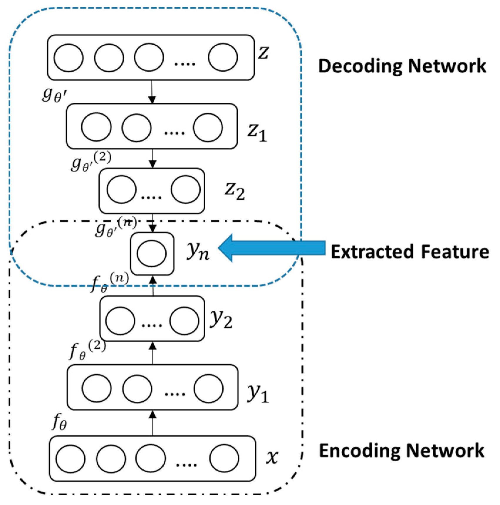
The DAE model consists of an input layer, hidden layer, and reconstruction unit layer, forming a three-layer symmetric structure unsupervised neural network. The first two layers form the encoding network, and the last two layers form the decoding network. The output of the hidden layer represents the feature extraction results of the single-layer DAE model.

The basic principle of the SDAE is as follows: Assuming the input data is $x$, a single-layer DAE will use a noise function $q_D$ to corrupt the input x and generate $x^{\prime }$. Then, through the encoding function $f_{\theta }$ , the noisy data $x^{\prime }$ is encoded into the feature $y_1$. After that, the decoding function ${ g}_{{\theta }^{\prime }}$ is used to obtain the reconstructed data $z$. The DAE parameters are trained by minimizing the reconstruction error $L_{H }(x,z)$, where $L_{H }(x,z)$ represents the squared difference loss function. By applying the trained encoding function $f_{\theta }$ to the features extracted from the hidden layer, denoted as $y_1$, and using it as the input for the next layer of DAEs, this process is repeated to train the stacked structure of SDAEs [25]. The structure of the SDAE model is the same as the DAE model, consisting of an encoding network and a decoding network, as shown in Figure 2.

2.3. The Process of Feature Extraction in the SDAE Method

The feature extraction process of the SDAE involves two stages: pre-training and fine-tuning. Firstly, the network parameters are initialized through unsupervised layer-wise pre-training. The output of each hidden layer in the encoding network represents the features extracted at each level during the pre-training process. Then, the network parameters are fine-tuned using back propagation and gradient descent algorithms to optimize the entire model. After the fine-tuning process is completed, the output of the last hidden layer in the encoding network corresponds to the features extracted by the SDAE network.

3. Fault Prediction Model Based on AGWO-GRU

3.1. GRU Model

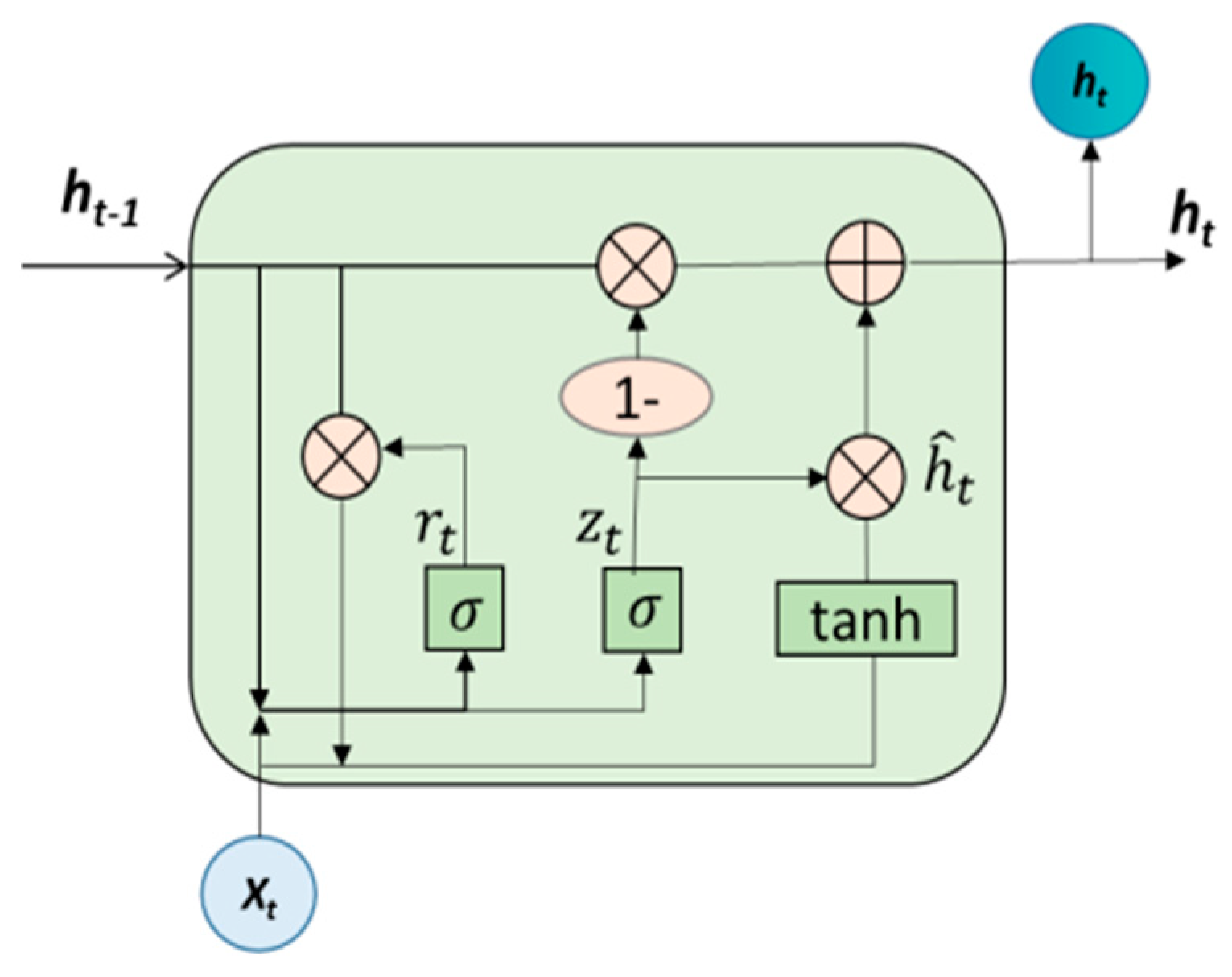
The failures of critical components in the output circuit of the signal conditioning module are attributed to continuous stress impacts, and these component failures exhibit time-dependence. Therefore, predicting circuit component failures can be transformed into a time-series forecasting problem. RNNs are neural networks with short-term memory capabilities and have found extensive applications in time-series prediction tasks. However, traditional RNNs suffer from issues such as vanishing gradients, exploding gradients, and a limited capability to process long-range data features. In order to address these problems, LSTM networks were introduced. LSTM networks incorporate gate mechanisms that enhance the memory capacity of the network, compensating for the limitations of traditional RNNs. Nevertheless, LSTM networks have drawbacks including long training times and a high parameter count. The GRU networks are a variant form of LSTM networks that combine the forget gate and input gate of LSTM networks into an update gate, reducing the number of gates and simplifying the network structure. While ensuring the memory capacity of neurons, GRU models improve the training speed of the model [26]. The structure of the GRU model is shown in Figure 3, primarily composed of an update gate $z_t$ and a reset gate $r_t$. The operational principle of a GRU network are shown in Equations (1)–(4):

$$\begin{array}{c}{r}_t=\sigma \left(W_r{x}_t+U_r{h}_{t-1}+b_r\right)\end{array}$$

(1)

$$\begin{array}{c}{z}_t=\sigma \left(W_z{x}_t+U_z{h}_{t-1}+b_z\right)\end{array}$$

(2)

$${\widehat{h}}_t=\tanh \left(W_h{x}_t+r_t{U}_h{h}_{t-1}+b_h\right)$$

(3)

$$\begin{array}{c}{h}_t=\left(1-z_t\right)h_{t-1}+z_t{\widehat{h}}_t \end{array}$$

(4)

where $x_t$ denotes the input at the current moment; $h_t$ denotes the output at the current moment; $h_{t-1}$ denotes the output at the previous moment; $r_t$ is the result of the reset gate activation; $z_t$ is the result of the update gate activation; ${\widehat{h}}_t$ denotes the candidate hidden state at the current moment; W, U denote the weight matrices; and b denotes the bias parameter.

3.2. AGWO Algorithm

The grey wolf optimization (GWO) algorithm has demonstrated excellent performance advantages in terms of solution accuracy and convergence speed, leading to its widespread application in network parameter optimization. Nonetheless, it often faces issues such as non-automated parameter tuning, a lack of systematic stop criteria, and a reliance on an empirically set maximum iteration count. These issues typically result in imbalanced exploration/exploitation and the inefficient use of computational resources. The AGWO algorithm addresses these problems by introducing adaptive adjustment strategies based on the fitness-based search stop criteria (threshold), significance threshold (ε), and exploration/exploitation parameter (a). This reduces the dependence on the iteration count and achieves automatic adjustment based on optimization behavior. Furthermore, the AGWO algorithm enhances optimization efficiency by enabling termination when the predefined search stop criteria and significance threshold conditions are satisfied. This prevents unnecessary computational time expenditure caused by negligible reductions in the objective function value [27]. The fundamental idea driving the AGWO algorithm is:

(1) Adaptive parameter tuning strategy: The parameter a used for the exploration/exploitation of the optimal position is adaptively adjusted based on the average fitness value of the objective function in historical iterations. The principle is shown in Equations (5)–(8):

$$\begin{array}{c}{F}_{movavg}^{\left(t\right)}={\displaystyle \frac{{\sum }_{t-w}^t{\overline{F}}^{\left(t\right)}}{w}}\end{array}$$

(5)

$${\overline{F}}^{\left(t\right)}<F_{movavg}^{\left(t-1\right)}-\epsilon$$

(6)

$$d=\gamma d$$

(7)

$$a=\left(1-k\right)a+k \ast d \ast \left(2\ast {\displaystyle \frac{\left|∆F_t\right|}{\left|∆F_{t-1}\right|}}\right)$$

(8)

whereas ${\overline{F}}^{\left(t\right)}$ represents the average fitness of the current iteration, $F_{movavg}^{\left(t\right)}$ represents the moving average fitness value constructed using a sliding window. N is the population size, w denotes the length of the moving average window, and i and t represent the current individual being optimized and the corresponding iteration, respectively. ε is the significance threshold indicator. When the decrease in ${\overline{ F}}^{\left(t\right)}$ compared to $F_{movavg}^{\left(t\right)}$ is greater than ε, it indicates that the parameter a has achieved a good pre-exploration/exploitation performance. Otherwise, the adaptive parameter a needs to be adjusted to reduce the exploration rate. d is an auxiliary parameter decayed by decay rate γ. k helps the parameter a maintain the previous exploration rate and change smoothly. $|∆F_t|$ represents the rate of change in the current iteration, and $|∆F_{t-1}|$ represents the rate of change in the previous iteration.

(2) Fitness-based search threshold stopping criteria:

The search stop criterion threshold is used to examine two conditions: the first, if the optimization process fails to improve the fitness value, and the second, if the adaptive parameter a used for exploration/exploitation becomes too small, hindering the wolf pack from exploring and adjusting to a more optimal search space. By setting a threshold for the search stop criterion, the search process can be terminated when either of these conditions is met. This helps reduce unnecessary exploration rates and allows the algorithm to focus on more promising areas for finding better solutions.

3.3. Signal Conditioning Module Fault Prediction Based on AGWO-GRU Model

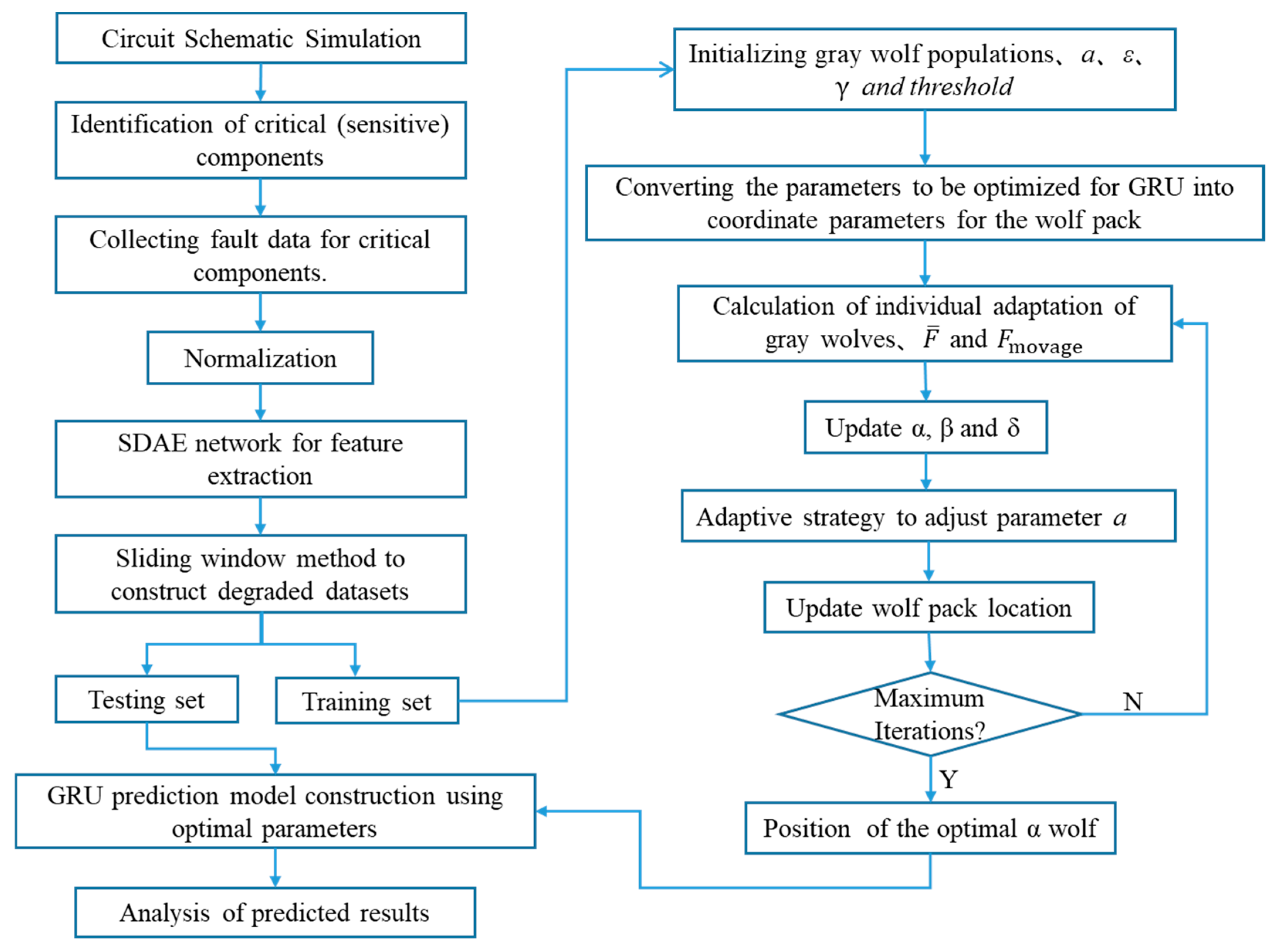
It is difficult to achieve accurate results by initializing the parameters of the GRU model through trial and error based on experience. Therefore, this paper proposes to use the AGWO algorithm to optimize the learning rate, number of hidden layers, and number of neurons in the hidden layers for the GRU model. Combining with the fault feature extraction method described earlier, this paper proposes a fault feature extraction method based on the SDAE and an improved AGWO-optimized GRU signal conditioning module prediction model. The AGWO-GRU failure prediction process is shown in Figure 4, and the specific implementation process is as follows:

(1)

Data acquisition: The signal conditioning module circuit is simulated and modeled using PSpice 17.4 simulation software, which allows for the identification of key components. Moreover, fault datasets are obtained during the simulation process for further analysis.

(2)

Data preprocessing: Normalize the collected fault data of critical components using min–max normalization.

(3)

Feature extraction using SDAE network: Train the normalized fault data using the SDAE network, and the output one-dimensional feature is the degradation feature of the component.

(4)

Constructing the fault dataset: Use the sliding window method to construct the extracted degradation features into training and testing sets that comply with the input format of the GRU model.

(5)

AGWO-optimized GRU model: Initialize the grey wolf population, take the learning rate of the GRU model, the number of hidden layers, and the number of hidden layer nodes as the coordinates of the position parameters of the wolves, select the training sample set to train the GRU, and obtain the position vector of the optimal α wolf which is the optimized GRU parameters.

(6)

Construct the GRU prediction model based on the optimized parameters, and input the testing set for prediction.

4. Simulation Modeling and Fault Prediction Verification of the Signal Conditioning Module’s Output Circuit

4.1. Simulation Modeling and Fault Data Acquisition

During normal operation, the signal processing module will experience a degradation in performance due to the increased years of usage and environmental stress. In terms of time progression, the signal processing module typically goes through three stages: the normal state, performance degradation state, and failure state. The signal conditioning module consists of three sub-modules: the power supply module, the signal input module, and the signal output module. The signal input module converts the received 4–20 mA current signal into a voltage signal, while the signal output module, as the core part of the board, mainly converts the isolated voltage signal into a current signal (V/I conversion). Therefore, this paper, based on the printed circuit board (PCB) hardware design schematics of the signal processing module, uses the PSpice simulation tool to complete the design and verification work for the signal output circuit, which includes the following:

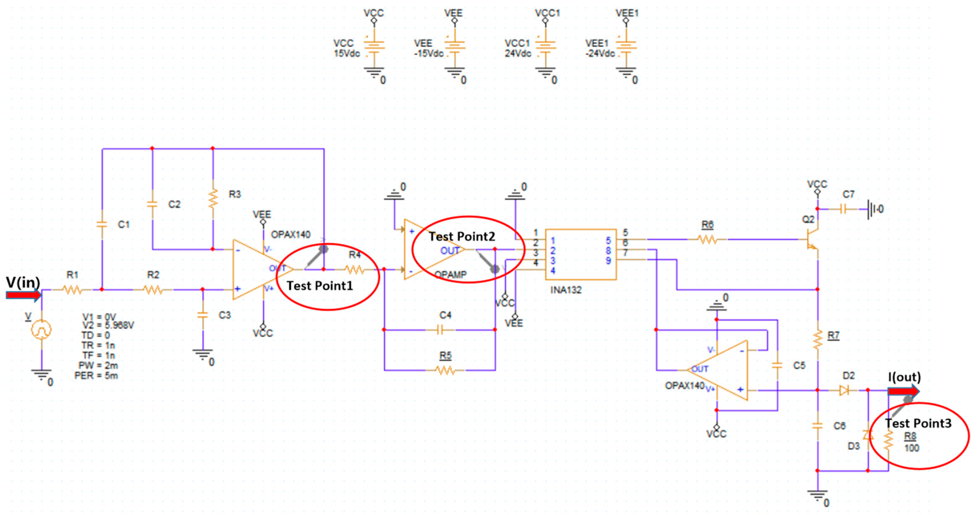
For the design part of the signal output circuit: A one-to-one simulation modeling is conducted based on the schematic diagram of the signal output circuit. The schematic of a certain DCS system’s signal output circuit is shown in Figure 5. The input signal of the signal output module is a voltage signal after I/V conversion, in which the current is converted to voltage in the signal input module, and the conversion equation is shown in Equation (9). In addition, three data recording points are placed on the simulation circuit model for the later monitoring of the circuit’s degradation status. Meanwhile, the nuclear safety-class signal conditioning module has the accuracy requirement that the error between the output current signal I_out of the signal output module and the input current signal I_in of the signal input module should be less than 0.2%. Therefore, this paper will follow this criterion to verify the effectiveness of the simulation circuit.

$$\begin{array}{c}\begin{array}{c}{\mathrm{V}}_{\mathrm{i}\mathrm{n}}=\mathrm{I} \ast 100 \ast 2.98\end{array}\end{array}$$

(9)

Validation of signal output circuit: Due to the simplification or approximation of the real module in the simulation model, the parameters, physical processes, or assumptions within the model may not accurately reflect the complexity or details of the actual module, thereby introducing simulation accuracy. Therefore, the simulation data need to be compared and validated against actual engineering measurements. Consequently, the validation of circuit outputs has been conducted for 4 mA, 8 mA, 12 mA, 16 mA, and 20 mA current signals, as well as 100 Ω, 300 Ω, and 600 Ω output loads. Each condition is measured four times, and averages are calculated to verify if the simulated circuit data meet the 0.2% design target accuracy. Concurrently, using actual engineering measurement values (referred to as actual value) as reference, the measurement error is defined as the percentage difference between the simulated circuit output values (referred to as simulation value) and the actual values. The comparison between the simulation data and actual engineering data is shown in

Table 1. Comparison of simulated and actual measured data.

	Load/Ω	CH1 /mA	CH2 /mA	CH3 /mA	CH4 /mA	AVG (CH1 to CH4)	Measurement Error	Accuracy
4 mA actual value	100	3.9974	3.9989	3.9984	3.9969	3.9979		0.2%
	300	3.9981	3.9989	3.9985	3.9969	3.9981		0.2%
	600	3.9980	3.999	3.9985	3.9969	3.9981		0.2%
4 mA simulation value	100					3.9963	0.040%	0.2%
	300					3.9962	0.047%	0.2%
	600					3.9961	0.051%	0.2%
8 mA actual value	100	7.9969	7.9983	7.9976	7.9938	7.9966		0.2%
	300	7.9974	7.9983	7.9977	7.9939	7.9968		0.2%
	600	7.9973	7.9985	7.9977	7.9938	7.9968		0.2%
8 mA simulation value	100					7.9925	0.052%	0.2%
	300					7.9923	0.057%	0.2%
	600					7.9920	0.060%	0.2%
12 mA actual value	100	11.9964	11.9979	11.9972	11.9908	11.9955		0.2%
	300	11.997	11.998	11.9971	11.9907	11.9957		0.2%
	600	11.9969	11.9984	11.9971	11.9908	11.9958		0.2%
12 mA simulation value	100					11.9887	0.057%	0.2%
	300					11.9884	0.061%	0.2%
	600					11.9879	0.065%	0.2%
16 mA actual value	100	15.9968	15.998	15.9974	15.9885	15.9951		0.2%
	300	15.9974	15.9983	15.9973	15.9885	15.9953		0.2%
	600	15.9971	15.9987	15.9973	15.9887	15.9954		0.2%
16 mA simulation value	100					15.9851	0.063%	0.2%
	300					15.9848	0.065%	0.2%
	600					15.9845	0.069%	0.2%
20 mA actual value	100	19.9981	19.999	19.9984	19.9869	19.9956		0.2%
	300	19.9984	19.9993	19.9984	19.9871	19.9958		0.2%
	600	19.9979	19.9993	19.9985	19.987	19.9956		0.2%
20 mA simulation value	100					19.9813	0.071%	0.2%
	300					19.9811	0.073%	0.2%
	600					19.9807	0.075%	0.2%

, where CH1, CH2, CH3, and CH4 represent the results of four actual and simulated measurements values, respectively, and AVG is the average of the four measurements. After validation, all simulated outputs meet the 0.2% accuracy requirement, confirming the effectiveness of the simulation results. Furthermore, compared to actual engineering measurements, the errors are all below 0.1%, indicating that the simulated data can effectively substitute for real experimental datasets.

The PSpice simulation tool is utilized to perform sensitivity analysis, evaluating the influence of parameter variations in different components of the circuit on the signal output. The resistors have a tolerance set at 0.01%, while the capacitors have a tolerance of 5%. Analysis reveals that variations in the parameters of feedback resistors R4 and R7, as well as filtering capacitors C1 and C3, significantly impact the functional performance of the circuit. In general, environmental factors like temperature and humidity cause resistors to exhibit increased resistivity, resulting in a unidirectional rise in resistance values. Conversely, capacitors experience a gradual decrease in capacitance value due to declining dielectric constants.

In this paper, the fault threshold values for four critical components in the signal conditioning module’s output circuit are determined based on the engineering specification that the error of the conditioned module’s output signal should be less than 0.2%. The failure threshold values for these four critical components are shown in

Table 2. Critical component failure threshold.

Component	Nominal Value	Tolerance	Threshold
R4	10 kΩ	0.01%	10.02 kΩ
R7	348 Ω	0.01%	348.7 Ω
C1	1 nF	5%	0.816 nF
C3	470 pF	5%	253.5 pF

. As shown in Table 2, the threshold for component R4 is 10.02 kΩ, for component R7 is 348.7 Ω, for component C1 is 0.816 nF, and for component C3 is 253.5 pF.

Using the PSpice simulation tool to perform a parameter sweep simulation on the above-mentioned four critical components, simulate the degradation process of individual components, and obtain the degradation data. A voltage pulse signal with a pulse width of 5 ms and an amplitude of 5.96 V is input from the voltage input port as the excitation signal of the circuit, and the current waveform at the data recording point is recorded, while the Monte Carlo mechanism is added to introduce random disturbances to improve the randomness of the data. It is assumed that the electrical parameters of the resistors and capacitors degrade linearly over time due to environmental stress. This degradation follows a uniform change from the nominal value of the component to the fault threshold value. The size of each change is 0.001% of its nominal value for resistive elements R4 and R7, and 0.092% for capacitive element C1 and 0.23% for C3. Following every parameter alteration, an excitation signal will be implemented, and the current waveforms at data recording points 1, 2, and 3 will be logged. Each component’s parameters will undergo 200 variations, resulting in the collection of 200 data samples for each component. Consequently, a total of 4 × 200 sets of data will be obtained. Moreover, each sample will consist of 500 sampling points.

4.2. Fault Feature Extraction of Signal Output Circuit

After obtaining the degradation data of the signal output circuit through PSpice simulation, the degradation features of each component are extracted using the stacked denoising autoencoder (SDAE) network. Firstly, the degradation data of each component are normalized using the min–max normalization method. Then, the normalized data are input into the SDAE network for feature extraction. The SDAE network structure used in this study for feature extraction is 500–100–20–1–20–100–500. The number of nodes in the input layer corresponds to the 500 sampling points at each time step of the component’s degradation data, and the output of the hidden layer with one node corresponds to the extracted fault features. The pre-training iterations and back propagation iterations of a single denoising auto encoder are set to 50, the noise rate is 0.01, the learning rate for resistors R4 and R7 is 1.5 × 10⁻⁴, and the learning rate for capacitors C1 and C3 is 1 × 10⁻⁶.

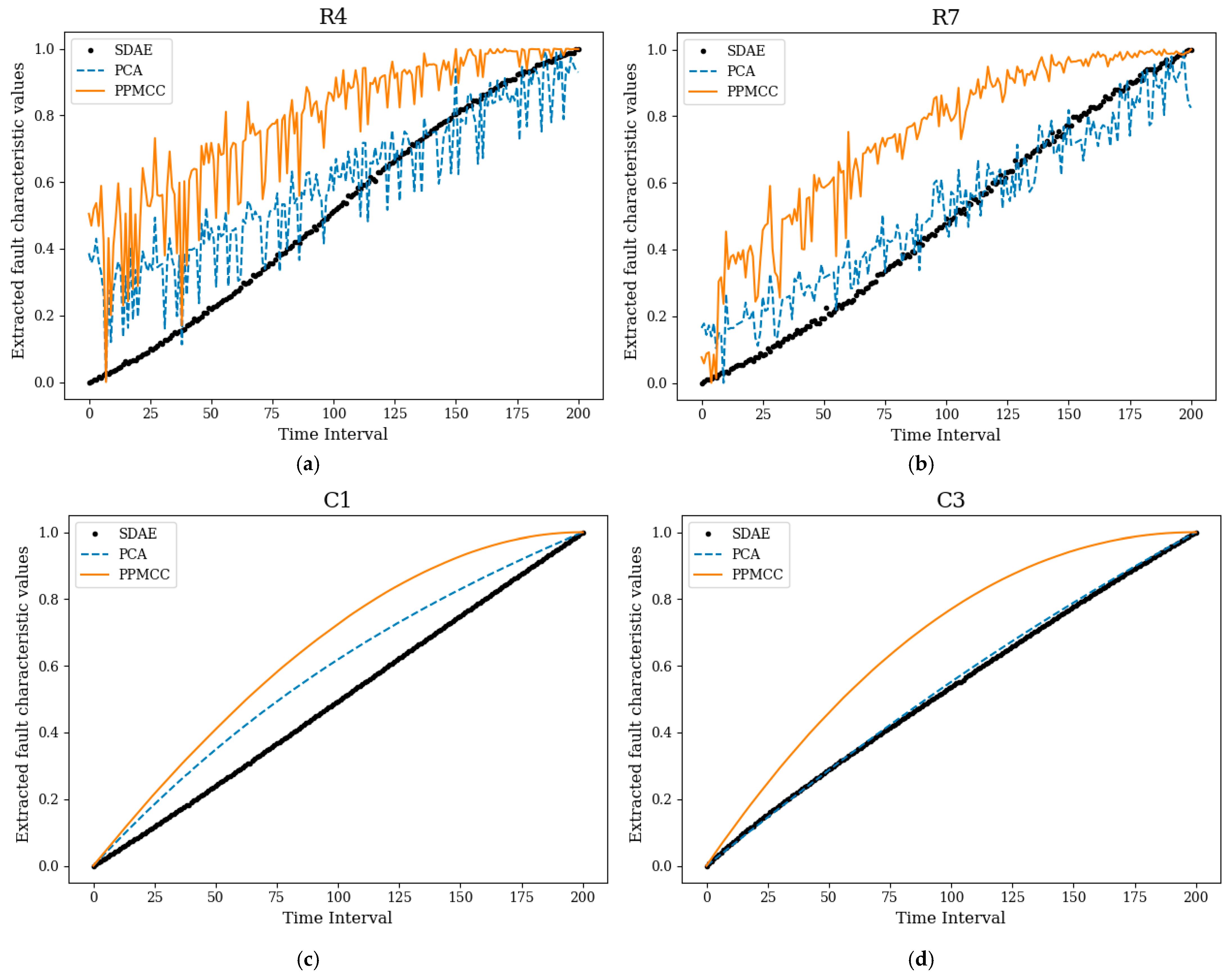
To validate the superiority of using the SDAE method for extracting minor deviation fault degradation features, a comparative analysis was conducted with the principal component analysis (PCA) method and Pearson product–moment correlation coefficient (PPMCC) method that combines the time–frequency domain features. The degradation feature extraction results for each component are shown in Figure 6a–d, where a fault feature value of 1 indicates that the circuit component has reached the fault threshold.

Evaluation metrics including time correlation and monotonicity are selected to analyze the feature extraction results [28]. The performance evaluation results of these three feature extraction methods for components R4, R7, C1, and C3 are presented in

Table 3. Comparison of feature extraction methods.

Component	Feature Extraction Method	Time Correlation	Monotonicity
R4	SDAE	0.9993	1
	PCA	0.9949	0.92
	PPMCC	0.9271	0.83
R7	SDAE	1	1
	PCA	0.9920	0.99
	PPMCC	0.9745	0.98
C1	SDAE	1	1
	PCA	0.9920	0.99
	PPMCC	0.9745	0.98
C3	SDAE	0.9994	1
	PCA	0.9985	0.99
	PPMCC	0.9617	0.97

. Based on the failure feature extraction results shown in Table 3, Figure 6a–d, it can be observed that, compared to the PPMCC method which combines time–frequency domain features and the PCA method, the method we proposed which is based on SDAE achieves a better performance in extracting minor deviation faults for components R4 and R7. Furthermore, the extracted degradation features are smoother and exhibit higher monotonicity.

Based on the feature extraction results shown in Table 3, it can be observed that, compared to the PPMCC method which combines time–frequency domain features and the PCA method, the method we proposed which is based on SDAE achieves a better performance in extracting minor deviation faults for components R4 and R7. The SDAE method achieves a time correlation of above 0.99 and a monotonicity of 1 for fault features extracted from components R4, R7, C1, and C3. Both the time correlation and monotonicity metrics are superior to those of the PCA and PPMCC methods. Moreover, Figure 6a–d indicate that, compared to the PCA and PPMCC methods, the SDAE-based approach yields fault features with smaller local noise and smoother curves. In summary, the method we proposed which is based on SDAE achieves a better performance in extracting minor deviation faults for components R4 and R7. Furthermore, the extracted degradation features are smoother and exhibit higher monotonicity.

4.3. Simulation Experiment Validation of AGWO-GRU Fault Prediction Model

After completing the fault feature extraction for each component using SDAE, the obtained fault features are used to construct a prediction sample set using the sliding window method with a window size of 5. The sample data were divided, with the first 50% being the training set used to train the AGWO-GRU fault prediction model, and the remaining 50% being the testing set used to evaluate the predictive performance of the model. The AGWO algorithm is applied to optimize the number of hidden layers, the number of nodes in each hidden layer, and the learning rate for the GRU model. The AGWO algorithm is configured with a grey wolf population of 10, a search stopping criterion threshold of 1 × 10⁻³, a significance threshold ε of 1 × 10⁻⁵, and a decay rate γ of 0.95.

The optimized parameters for the GRU model are shown in

Table 4. Optimized parameters of GRU model.

Input Layer Nodes	Number of Hidden Layer	Hidden Layer Nodes	Learning Rate	Output Layer Nodes
5	1	103	2.45 × 10−3	1

. From Table 4, it can be observed that the optimized GRU model has five nodes in the input layer, one node in the output layer, and a learning rate of 2.45 × 10⁻³, with only one hidden layer containing 103 nodes.

The GRU prediction model is constructed using optimized parameters. In order to validate the superiority of the proposed method, the prediction results of the AGWO-GRU model, LSTM model, RNN model, SVM, MKRVM, and PF are compared and analyzed using the same data. The parameters of the RNN and LSTM models are the same as those of the GRU model. The comparison of prediction methods on the testing sets for components R4, R7, C1, and C3 are shown in Figure 7a–d. Evaluation metrics including the root mean square error (RMSE), mean absolute error (MAE), mean absolute percentage error (MAPE), and absolute error (EA) are selected to analyze the prediction results [19]. The performance evaluation results of these six prediction methods for components R4, R7, C1, and C3 are presented in

Table 5. Comparison of prediction performance of different methods.

Component	Method	RMSE	MAE	MAPE	EA	Accuracy
R4	PF	1.22 × 10−4	0.0098	1.2432	0.007951	99.20%
	SVM	1.12 × 10−4	0.0096	1.1447	0.014541	98.55%
	MKRVM	1.78 × 10−5	0.0032	0.4054	0.000606	99.94%
	RNN	8.59× 10−4	0.0155	2.4552	0.004006	99.60%
	LSTM	4.52 × 10−5	0.0133	1.5292	0.003213	99.68%
	AGWO-GRU	1.47 × 10−5	0.0029	0.3905	0.000109	99.99%
R7	PF	5.17 × 10−4	0.0196	2.6708	0.023256	97.67%
	SVM	1.92 × 10−4	0.0118	2.5066	0.019266	98.07%
	MKRVM	1.06 × 10−4	0.0094	1.2007	0.000798	99.92%
	RNN	8.62 × 10−4	0.0190	2.9768	0.000717	99.93%
	LSTM	1.88 × 10−5	0.0106	1.0986	0.000438	99.96%
	AGWO-GRU	7.21 × 10−5	0.0065	0.6321	5.33 × 10−5	99.99%
C1	PF	1.39 × 10−4	0.0054	0.8772	0.007598	99.24%
	SVM	8.67 × 10−5	0.0046	0.6417	0.002098	99.79%
	MKRVM	2.43 × 10−5	0.0022	0.2791	0.000279	99.97%
	RNN	2.59 × 10−4	0.0063	1.0417	0.000540	99.95%
	LSTM	3.03 × 10−5	0.0050	0.7265	0.000231	99.98%
	AGWO-GRU	1.83 × 10−6	0.0011	0.1418	0.000102	99.99%
C3	PF	8.82 × 10−5	0.0056	0.8643	0.002718	99.73%
	SVM	4.02 × 10−5	0.0054	0.7512	0.000754	99.92%
	MKRVM	5.56 × 10−5	0.0048	0.6327	0.000234	99.97%
	RNN	1.25 × 10−4	0.0061	1.3213	0.000592	99.94%
	LSTM	3.29 × 10−5	0.0051	0.7274	7.72×10-5	99.99%
	AGWO-GRU	1.49 × 10−5	0.0035	0.4936	3.65×10-5	99.99%

. And the comparison of the training time and testing time between the AGWO-GRU model and the LSTM model is shown in

Table 6. Comparison of training/testing time.

Component	Method	Training Time/s	Testing Time/s
R4	LSTM	36.83992	0.0080020
	AGWO-GRU	2.70715	0.0060019
R7	LSTM	35.57344	0.0070014
	AGWO-GRU	2.20703	0.0050010
C1	LSTM	14.72103	0.010002
	AGWO-GRU	0.56013	0.0060009
C3	LSTM	12.04802	0.0080018
	AGWO-GRU	0.46063	0.0070018

.

Figure 7a–d depict the prediction results on components R4, R7, C1, and C3 using various methods, including GWO-GRU, LSTM, RNN, PF, SVM, and MKRVM. It can be seen from the figures that, compared to the PF, SVM, MKRVM, LSTM, and RNN prediction models, the proposed AGWO-GRU prediction model exhibits less fluctuation in the prediction curves on the test set and achieves better fitting. According to Table 5, the AGWO-GRU method achieves a prediction accuracy of 99.99%, which is higher compared to PF, SVM, MKRVM, LSTM, and RNN, and it also shows a lower RMSE, MAE, MAPE, and EA. Furthermore, Table 6 demonstrates that, compared to the LSTM model, the proposed AGWO-GRU model operates with shorter execution times on both the training and test sets, indicating higher operational efficiency. In summary, these findings suggest that the proposed AGWO-GRU prediction model offers superior prediction accuracy, better time performance, and enhanced generalization capabilities, thereby enabling the more accurate prediction of circuit fault severity.

5. Conclusions

This paper proposes a fault prediction method based on SDAE feature extraction and AGWO-GRU to address the problems of insufficient feature extraction accuracy, low fault prediction accuracy, and poor dynamic adaptability for minor deviations in high-precision devices in existing nuclear power plants. The safety-class signal conditioning module output circuit is selected as the research object, and fault simulation modeling is carried out based on the circuit schematic to simulate the degradation process of key circuit components, thereby obtaining degradation datasets. The SDAE method is used to extract the fault features of key components, and the extracted fault features are used as inputs for the fault prediction model. The AGWO algorithm is used to optimize the number of hidden layers, hidden layer nodes, and learning rate of the GRU prediction model; and the optimized GRU model is used for prediction and compared with the prediction results of the RNN, LSTM, PF, SVM, and MKRVM models. Through a comparative analysis of different models, the following conclusions can be drawn:

• The SDAE-based feature extraction method proposed in this paper achieves smoother, better trending, and more reflective fault features of component degradation without relying on expert experience and complex signal processing technology, surpassing the PCA method and traditional signal feature extraction methods.
• The AGWO-GRU model proposed in this paper has a higher prediction accuracy compared to the RNN, LSTM, PF, SVM, and MKRVM models. It accurately predicts the future trend of circuit fault features and demonstrates improved stability. The AGWO algorithm optimization enhances the dynamic adaptability of the prediction model.
• The proposed model accurately predicts faults in the safety-class signal conditioning module even with limited monitoring data. It exhibits a good long-term prediction performance, providing valuable insights for the monitoring and operation and maintenance of electronic equipment in complex environments of nuclear power plants.
• The universality of SDAE-based fault feature extraction needs further verification as there may be uncertainties when using degradation data from the safety-class signal conditioning module to evaluate the performance degradation of other electronic equipment in nuclear power plants.
• Future research should consider the diversity and stage characteristics of degradation modes and further study the structure of prediction models. The focus should be on multi-component degradation faults as this study only investigated single-component degradation faults.

In summary, the proposed fault prediction method based on SDAE feature extraction and AGWO-GRU shows promising results in addressing the challenges of minor fault prediction in high-precision devices in nuclear power plants. Further research and validation are necessary to explore the applicability of this method across different electronic devices and degradation scenarios.

References

1. Perrow, C. Normal accident at three mile island. Society 1981, 18, 17–26. [Google Scholar] [CrossRef]
2. Zhao, S.; Chen, S.; Yang, F.; Ugur, E.; Akin, B.; Wang, H. A composite failure precursor for condition monitoring and remaining useful life prediction of discrete power devices. IEEE Trans. Ind. Inform. 2020, 17, 688–698. [Google Scholar] [CrossRef]
3. Cheng, Y.; Wang, C.; Wu, J.; Zhu, H.; Lee, C.K. Multi-dimensional recurrent neural network for remaining useful life prediction under variable operating conditions and multiple fault modes. Appl. Soft Comput. 2022, 118, 108507. [Google Scholar] [CrossRef]
4. Hu, G.; Zhou, T.; Liu, Q. Data-driven machine learning for fault detection and diagnosis in nuclear power plants: A review. Front. Energy Res. 2021, 9, 663296. [Google Scholar] [CrossRef]
5. Liu, J.; Seraoui, R.; Vitelli, V.; Zio, E. Nuclear power plant components condition monitoring by probabilistic support vector machine. Ann. Nucl. Energy 2013, 56, 23–33. [Google Scholar] [CrossRef]
6. Do Koo, Y.; Jo, H.S.; Na, M.G.; Yoo, K.H.; Kim, C.H. Prediction of the internal states of a nuclear power plant containment in LOCAs using rule-dropout deep fuzzy neural networks. Ann. Nucl. Energy 2021, 156, 108180. [Google Scholar] [CrossRef]
7. Chen, Y.; Yuan, J.; Luo, Y.; Zhang, W. Fault prediction of centrifugal pump based on improved KNN. Shock. Vib. 2021, 2021, 1–12. [Google Scholar] [CrossRef]
8. Chen, H.; Gao, P.; Tan, S.; Yuan, H.; Guan, M. Prediction of Automatic Scram during Abnormal Conditions of Nuclear Power Plants Based on Long Short-Term Memory (LSTM) and Dropout. Sci. Technol. Nucl. Install. 2023, 2023, 2267376. [Google Scholar] [CrossRef]
9. Rathnapriya, S.; Manikandan, V. Remaining useful life prediction of analog circuit using improved unscented particle filter. J. Electron. Test. 2020, 36, 169–181. [Google Scholar] [CrossRef]
10. Hu, W.; Zhu, X.; Fan, H.; Liu, J. A novel method for analog circuit fault prediction based on IAALO-SVM[C]//12th International Conference on Quality, Reliability, Risk, Maintenance, and Safety Engineering (QR2MSE 2022). IET 2022, 2022, 1676–1682. [Google Scholar]
11. Wang, L.; Shi, L. Fault prediction for analog circuits based on improved correlation vector machines. Comput. Appl. Softw. 2023, 40, 52–60. [Google Scholar]
12. Hu, J. Research on Analog Circuit Fault Prediction Method Based on Deep Learning. Master’s Thesis, Zhengzhou University, Zhengzhou, China, 2021. [Google Scholar] [CrossRef]
13. Sun, S.; Wang, Z.; Wang, J.; Yang, F.; Ji, W. Remaining Useful Life Prediction for Circuit Breaker Based on SM-CFE and SA-BiLSTM. IEEE Trans. Instrum. Meas. 2023, 72, 1–14. [Google Scholar] [CrossRef]
14. Zhang, C.; He, Y.; Yuan, L.; Xiang, S. Analog Circuit Incipient Fault Diagnosis Method Using DBN Based Features Extraction. IEEE Access 2018, 6, 23053–23064. [Google Scholar] [CrossRef]
15. Cao, H.; Sun, P.; Zhao, L. PCA-SVM method with sliding window for online fault diagnosis of a small pressurized water reactor. Ann. Nucl. Energy 2022, 171, 109036. [Google Scholar] [CrossRef]
16. Wang, Y.; Wu, D.; Yuan, X. LDA-based deep transfer learning for fault diagnosis in industrial chemical processes. Comput. Chem. Eng. 2020, 140, 106964. [Google Scholar] [CrossRef]
17. Liu, X.; Zhang, Z.; Meng, F.; Zhang, Y. Fault diagnosis of wind turbine bearings Based on CNN and SSA–ELM. J. Vib. Eng.Technol. 2022, 11, 3929–3945. [Google Scholar] [CrossRef]
18. Su, X.; Cao, C.; Zeng, X.; Feng, Z.; Shen, J.; Yan, X.; Wu, Z. Application of DBN and GWO-SVM in analog circuit fault diagnosis. Sci. Rep. 2021, 11, 7969. [Google Scholar] [CrossRef]
19. Jiang, Z. Fault Diagnosis and Prediction of Analog Filters Based on Deep Learning. Master’s Thesis, Harbin Institute of Technology, Harbin, China, 2019. [Google Scholar] [CrossRef]
20. Du, X.; Jia, L.; Haq, I.U. Fault diagnosis based on SPBO-SDAE and transformer neural network for rotating machinery. Measurement 2022, 188, 110545. [Google Scholar] [CrossRef]
21. Bengio, Y.; Courville, A.; Vincent, P. Representation learning: A review and new perspectives. IEEE Trans. Pattern Anal. Mach. Intell. 2013, 35, 1798–1828. [Google Scholar] [CrossRef] [PubMed]
22. Suk, H.I.; Lee, S.W.; Shen, D.; Alzheimer’s Disease Neuroimaging Initiative. Latent feature representation with stacked auto-encoder for AD/MCI diagnosis. Brain Struct. Funct. 2015, 220, 841–859. [Google Scholar] [CrossRef]
23. Hong, C.; Chen, X.; Wang, X.; Tang, C. Hypergraph regularized autoencoder for image-based 3D human pose recovery. Signal Process. 2016, 124, 132–140. [Google Scholar] [CrossRef]
24. Vincent, P.; Larochelle, H.; Lajoie, I.; Bengio, Y.; Manzagol, P.A.; Bottou, L. Stacked denoising autoencoders: Learning useful representations in a deep network with a local denoising criterion. J. Mach. Learn.Res. 2010, 11, 3371–3408. [Google Scholar]
25. Yan, X.; Liu, Y.; Jia, M. Health condition identification for rolling bearing using a multi-domain indicator-based optimized stacked denoising autoencoder. Struct. Health Monit. 2020, 19, 1602–1626. [Google Scholar] [CrossRef]
26. Zhang, Y.G.; Tang, J.; He, Z.Y.; Tan, J.; Li, C. A novel displacement prediction method using gated recurrent unit model with time series analysis in the Erdaohe landslide. Nat. Hazards 2021, 105, 783–813. [Google Scholar] [CrossRef]
27. Meidani, K.; Hemmasian, A.; Mirjalili, S.; Barati Farimani, A. Adaptive grey wolf optimizer. Neural Comput. Appl. 2022, 34, 7711–7731. [Google Scholar] [CrossRef]
28. Binu, D.; Kariyappa, B.S. Rider-deep-LSTM network for hybrid distance score-based fault prediction in analog circuits. IEEE Trans. Ind. Electron. 2020, 68, 10097–10106. [Google Scholar] [CrossRef]
Figure 1. (a) DAE model structure. (b) Schematic diagram of DAE model.
Energies 17 04063 g001
Figure 2. SDAE model structure.
Energies 17 04063 g002
Figure 3. GRU model structure.
Energies 17 04063 g003
Figure 4. AGWO-GRU failure prediction process.
Energies 17 04063 g004
Figure 5. Signal output circuit schematic.
Energies 17 04063 g005
Figure 6. (a) Feature extraction results for R4. (b) Feature extraction results for R7. (c) Feature extraction results for C1. (d) Feature extraction results for C3.
Energies 17 04063 g006
Figure 7. (a) Comparison of prediction methods on R4. (b) Comparison of prediction methods on R7. (c) Comparison of prediction methods on C1. (d) Comparison of prediction methods on C3.
Energies 17 04063 g007