Article

Predicting Energy Production in Renewable Energy Power Plants Using Deep Learning

by
Abdil Karakan
Electrical Department, Dazkırı Vocational School, Afyon Kocatepe University, Afyonkarahisar 03204, Turkey
Energies 2024, 17(16), 4031; https://doi.org/10.3390/en17164031
Submission received: 13 July 2024 / Revised: 9 August 2024 / Accepted: 13 August 2024 / Published: 14 August 2024
(This article belongs to the Section F3: Power Electronics)

Abstract

:
It is very important to analyze and forecast energy production for investments in renewable energy resources. In this study, the energy production of wind and solar power plants, which are among the leading renewable energy sources, was estimated using deep learning. For a solar power plant, three different solar power plants with 1MW installed power were examined. Three-year energy production data of power plants were taken. These data were used with the deep learning method long short-term memory (LSTM) and seasonal autoregressive moving average (SARIMA). Results were obtained for each dataset; they were subjected to five different (MSE, RMSE, NMSE, MAE, and MAPE) error performance measurement systems. In the LSTM model, the highest accuracy rate was 81% and the lowest accuracy rate was 59%. In the SARIMA model, the highest accuracy rate was 66% and the lowest accuracy rate was 41%. As for wind energy, wind speeds in two different places were estimated. Wind speed data were taken from meteorological stations. Datasets were tested with MAPE, R2, and RMSE error performance measurement systems. LSTM, GRU, CNN-LSTM, CNN-RNN, LSTM-GRU, and CNN-GRU deep learning methods were used in this study. The CNN-GRU model achieved a maximum accuracy of 99.81% in wind energy forecasting.

1. Introduction

Renewable energy is a term used for energy sources, such as solar, wind, biomass, geothermal, hydroelectricity, and wave energy. Renewable energy systems are a set of systems used to meet the electricity needs due to the decrease in resources, such as natural gas and coal. Fossil fuels and their derivatives, which are frequently used in electricity generation, not only pollute the environment but also have negative effects on human, animal, and plant health. For similar reasons, the use of renewable energy is important. The demand for these existing renewable energy resources is increasing day by day. However, not enough studies on energy efficiency have been conducted. This situation creates a significant obstacle against fossil fuels. The initial installation and maintenance costs of solar power plants are high. However, considering that their average lifespan is 25 years, the issue of efficiency is significant for solar power plants. There are many studies on solar energy systems [1,2,3,4,5]. Wang and his colleagues worked on estimating solar energy using power data and meteorological data. In their studies, they proposed three different methods: convolutional neural network (ESA), UKSB, and ESA-UKSB hybrid model. The performances of the forecast models were compared using datasets created with six-month periods [6]. In their study, Yıldız and Açıkgöz proposed a Kernel overlearning machine-based method for solar energy estimation. The proposed model demonstrated superior prediction performance compared to the extreme learning machine (ELM) and Levenberg–Marquardt-based methods used as a comparison method. This was proven by performance criterion values [7]. In their study, Li and his colleagues proposed a hybrid model created by the combination of the Wavelet Packet Decomposition (WPD) method and UKSB for solar energy forecasting. The power data obtained from the power plant were separated into their components via the WPD method. Performance evaluation results showed that the proposed hybrid model is more successful than models based on multilayer sensors [8]. In their study, Behera and his colleagues proposed three different hybrid methods obtained as a result of the combination of particle swarm optimization methods and the ALM method. Additionally, the GYSA-based method was used as a comparison method. Three different datasets were obtained using solar energy output power data measured at 15, 30 and 60 min intervals. The results obtained at different time horizons for the short-term prediction of solar energy showed that the hybrid model, which is a combination of accelerated particle swarm optimization and ALM, exhibited superior prediction performance compared to other models. Proven by performance evaluation results, it has been stated that hybrid ALM models give better prediction results than the comparison method for all datasets [9]. In a study by Su et al., the last ten neural networks were analyzed for short-term PV prediction. It was suitably calibrated and evaluated on a one-year dataset of a 406 MWp PV plant in the UK. Additionally, a new hybrid forecasting strategy derived as the sum of the best-performing forecasting models is proposed and evaluated. They concluded that among all the methods, the proposed hybrid model generally showed the best performance [10]. Mishra et al. proposed a WPD-UKSB-based method in their study. With the WPD method, time-series solar energy data were separated into different frequency series and used in the dataset. The dataset was organized in two different ways. The results obtained to predict the time horizon one hour ahead showed that the proposed deep learning-based method had better prediction performance than the machine learning-based methods used as a comparison method. This has been proven by performance evaluation results [11].
Forecasting wind energy is of vital importance in the process of determining energy production strategies. However, this process covers a very complex and challenging application area. Researchers have adopted various methods to overcome this challenge. At the same time, they have constantly tried to develop new approaches [12,13,14,15,16,17,18]. In a study conducted by Tan, a hybrid prediction model consisting of four modules, clustering, data pre-processing, evaluation, and prediction, was proposed. Performance analysis was made by comparing the results obtained with the proposed model with the results of some traditional prediction models [19]. In a study conducted by Görgel and Kavlak, hybrid CNN and LSTM methods were used, and energy production estimates were made. Apart from the hybrid method, the CNN, LSTM, and GRU methods were applied one by one for comparison purposes, and the results were shown graphically. The mean square error in production prediction made with the developed hybrid CNN-LSTM learning structure was reduced to 1.17 [20,21,22]. Transmission Systems Operators (TSOs) in Europe are helping power plants develop their planning strategies by publishing wind forecasts ahead of daily market clearing. Toubeau and his colleagues developed a new deep learning method with the idea that more effective results can be obtained by combining the prediction results of more than one model for large-scale planning [23]. Azad and colleagues developed two fundamentally different approaches, namely statistical and neural network-based approaches, to predict the following year’s hourly wind speed data. They used a set of recent wind speed measurement samples from two meteorological stations in Malaysia, namely Kuala Terengganu and Mersing, to train and test the dataset. The results obtained with the proposed method gave very promising results in terms of a very small mean absolute error (MAE) [24]. Tascıkaroglu and his colleagues used wavelet transform (WT) to decompose wind speed data into more stationary components. They later proposed a new wind speed estimation method that uses a spatiotemporal model in each subseries to include both temporal and spatial information [25]. To improve the accuracy of wind speed and wind power prediction, an ultra-short-term wind speed prediction model based on time-scale recognition and dynamic adaptive modeling is proposed. It shows that the proposed model offers higher accuracy than benchmark models that use the same prediction algorithms without considering the time scale and data sweep [26]. Wang et al. proposed a multi-mode multi-task transformer network (M2TNet) model that can achieve ultra-short-term wind power multi-step forecasting based on multi-source heterogeneous data, which confirmed that the M2TNet model performs better in terms of prediction accuracy and computational efficiency [27]. Wind speed measurement is not always performed on land. Wind speed forecasts are also made at ports. By estimating wind speed in ports, port operations are ensured on time, and efficiency in energy use is increased. Gu and colleagues proposed a wind speed prediction model based on the Sparrow Search Algorithm (SSA) optimized Wavelet Neural Network (WNN) to obtain high accuracy and fast prediction of harbor wind speed. To verify the effectiveness of the proposed method, the model is validated using wind speed data measured from the Chuanshan Port Area of Ningbo-Zhoushan Port during 2022, and its performance is compared with three other models: SSA–BP, SSA–LSTM, and WNN. It reveals that the proposed forecasting model has a good performance in port wind speed forecasting and outperforms other comparative models in terms of forecasting accuracy and convergence speed [28]. In their study, Lin et al. used the temporal convolution network (TCN) algorithm to predict long-term wind power with a MAPE of less than 10%. In the study, a MAPE value of 5.13% was obtained for a 72 h wind power forecast. Finally, measurements were made with the LSTM, RNN, and GRU models for power estimation and compared with TCN results [29].
In this study, forward-looking electricity production predictions were made using renewable energy sources, artificial intelligence, and deep learning. In our study, the LSTM and SARIMA models, one of the deep learning methods, were used. Three different regions with an annual production capacity of 1 MW were selected as examples. They were analyzed over three SPPs. As for wind energy, wind speeds in two different places were estimated. As a result of this study, weekly, monthly, and annual predictions were made. Tests were conducted with the MAPE, R2, and RMSE error performance measurement systems. The LSTM, GRU, CNN-LSTM, CNN-RNN, and LSTM-GRU deep learning methods were used in this study. The CNN-GRU model achieved high success in wind energy forecasting.
The most important advantage of this study is the dataset. A unique and new dataset was prepared for this study. The dataset was obtained from three different real solar power plants. Three years’ worth of data was taken to achieve high accuracy in this study. Considering that the lifespan of solar power plants is 25 years, 3 years of data is thought to be at the optimum level. Two different models and five different performance evaluation measurement systems were used in this study. In this way, a high accuracy of 89% was achieved. The energy efficiency of power plants will decrease over the years. By estimating the production values of the power plant, it is possible to carry out plant maintenance at the most appropriate time and at a low cost.
The structure of this article is as follows: Section 2 introduces the principles of LSTM and SARIMA, which are solar and wind speed prediction algorithms, the steps of the optimization algorithm, and the datasets. Section 3 estimates the 2023 energy production of solar power plants at three different points and the annual, monthly and weekly energy production of wind power plants at two different points. It analyzes the prediction results and verifies the effectiveness and superiority of the proposed method. Finally, Section 4 concludes this paper.

2. Materials and Methods

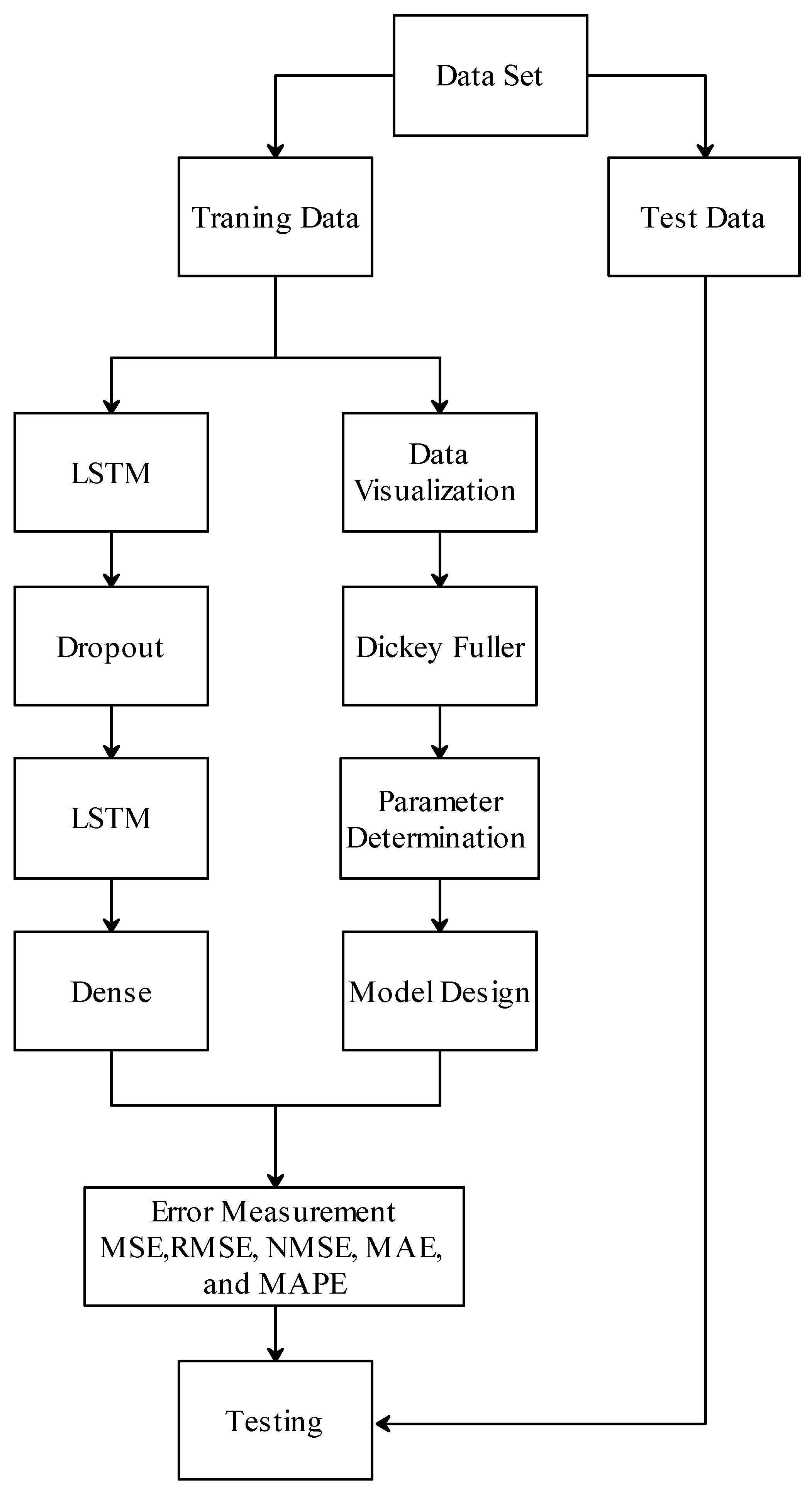
LSTM and SARIMA models were used in this study. The data used in these models are univariate time series. MSE, RMSE, NMSE, MAE, and MAPE error measurements were used to compare the prediction accuracies of these models. A basic flow diagram of the LSTM and SARIMA models used in this study is shown in Figure 1.

2.1. LSTM Model

The sequential basis model available in the Keras library was preferred. Among the layers of this model, the LSTM model was mainly used. The general structure of the model is shown in Table 1.
The model has a structure consisting of four layers. In the first layer, the number of inputs for LSTM was determined as 32. The tracking layer was added because forgetting weak information returns a positive result for the prediction mechanism. The value is given as 0.5. After the dilution process, a new LSTM layer was created in the third layer. The number of intermediate entries was determined as 25. Finally, the dense layer was added as an artificial neural network model. The output size is given as 1. ReLU was used as the activation function. RMSProp algorithm was added for optimization. Batch size was given as 16. Each step was 200 epochs. The standard LSTM model was used.

2.2. SARIMA Model

Python V 3.8.0.-supported Statsmodels library was used to create this model. In addition, the pmdarima library was used to find SARIMA parameters in the most appropriate way in SPPs containing daily data. In addition, the most suitable model was selected among different models using the AIC method. It is a process that requires statistical attention to determine the parameters during the working process of the SARIMA model. For this purpose, apart from AIC, the Dickey–Fuller unit root test was applied to check whether the time series ensured stationarity. This test is a method developed for the detection of stationary or non-stationary time series. Whether time series contain unit roots can be found with this test. In SARIMA, it is recommended to run the forecasting mechanism on stationary time series. Non-stationary time series must be made stationary to determine the parameters [30,31,32].

2.3. Performance Measurements

The performance of forecasting methods is measured by various metrics related to forecast error. Higher error values mean lower prediction accuracy. Some commonly used performance metrics were used to calculate the prediction error [33].

2.3.1. Mean Square Error

The mean square error (MSE) describes the distance between a regression curve and a set of points. MSE measures the performance of a machine learning model’s prediction mechanism. It always has a positive value. The closer the MSE result is to zero, the better the prediction mechanism performs. The mathematical equation of the MSE performance metric is shown below.
M S E = 1 n i = 1 n ( x ˜ i x i ) ²

2.3.2. Normalized Mean Square Error

Normalized mean square error (NMSE) is the normalized version of MSE. NMSE measured for the best model is closest to zero. In this case, the model is considered to be successful [34]. The mathematical equation of the NMSE performance metric is shown below.
N M S E = n i = i n ( x ˜ i x i ) ² i = i n x i i = i n x ˜ i

2.3.3. Root Mean Square Error

Root mean square error (RMSE) is found by taking the square root of MSE. It is a quadratic measurement used to find the distance between the value predicted by the prediction mechanism of a machine learning model and the actual values. RMSE describes the standard deviation of forecast errors. In other words, residuals are a measure of how far the regression line is from the actual data points. It does not allow for the use of absolute values, which are undesirable in many mathematical calculations. By definition, the closer RMSE is to 0, the better fit it is with the data. However, in practice, it never takes the value 0. In general, a lower RMSE is better than a higher one. Because RMSE depends on the scale of the numbers used as measurements, comparisons between different types of data will not be valid. It is frequently used in model comparisons. The mathematical equation of the RMSE performance metric is shown below.
R M S E = 1 n i = 1 n ( x ˜ i x i ) ²

2.3.4. Mean Absolute Error

Mean absolute error (MAE) is a measure of the difference between two continuous variables. MAE is the average vertical distance between each true value and the line that best fits the data. It is also the average horizontal distance. The MAE result is easily interpretable and is frequently used in regression and time-series problems. The mathematical equation of the MAE performance metric is shown below.
M A E = 1 n i = 1 n | x ˜ i x i |

2.3.5. Average Absolute Percent Error

Mean absolute percent error (MAPE) is used in regression and time-series models. MAPE is often preferred to determine the accuracy of predictions. If the real values contain zero, MAPE cannot be calculated because they will be divided by zero. For very low predicted values, the percentage error cannot exceed 100%. However, when very high prediction values are produced, there is no upper limit to the percentage error. MAPE is used to compare the accuracy of models used in prediction.
MSE, RMSE, NMSE, MAE, and MAPE methods were used for predictive performance measurements for the solar power plant data used in our study. The mathematical equation of the MAPE performance metric is shown below.
M A P E = 1 n i = 1 n | x ˜ i x i x i | × 100 %

2.3.6. ARIMA Parameter

The autoregressive integrated moving average model is used in non-stationary time series. It uses the Box–Jenkins method. Although they represent differences in local trends or levels, different parts of non-stationary processes show some degree of similarity in time series. A constant ARIMA (m, d, n) model with a difference is represented by the following equation.
x ˜ t = i = 1 m Φ s d x t 1 + j = 1 n θ j ω t j
Here, S = 1 − q − 1 and Φm (q) are a constant and reversible AR (m) operator. Xt, ωt, Φt and θj are the observed time-series values, error, AR, and MA values, respectively. d is the number of non-seasonal differences; m is the number of autoregressive terms; and n is the number of lagged forecast errors.

2.4. Dataset

In this study, three datasets belonging to solar power plants located in different locations and each with an installed power of 1MW were examined. Each of these three datasets contains a total of three years of electricity production data (kWh), with daily frequencies. These data consist of univariate time series. The coordinates of the first solar energy production power plant examined in this study are 37°45′78″ N, 32°69′18″ E, the coordinates of the second power plant are 37°96′62″ N, 32°72′94″ E, and the coordinates of the third power plant are 37°39′24″ N is 30°40′16″ E.
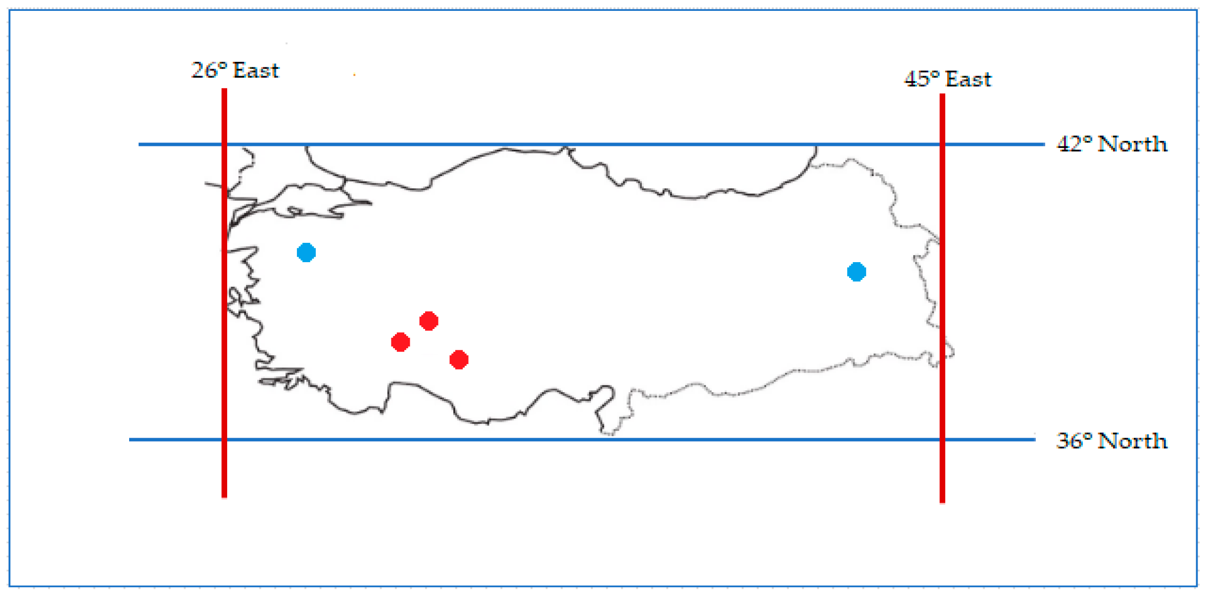
As for wind energy, wind speeds in two different places were estimated. The coordinates of the first wind energy production power plant examined in this study are 40°18′88″ N, 30°03′74″ E, and the coordinates of the second power plant are 38°44′50″ N, 42°83′05″ E. Wind speed changes in two different places were taken from the data at the meteorological station. Thus, 2-year data taken from the meteorological station were used. In Figure 2, the red dots show the location of solar energy systems, and the blue dots show the location of wind energy.

3. Result and Discussion

3.1. Predictions for Solar Energy System

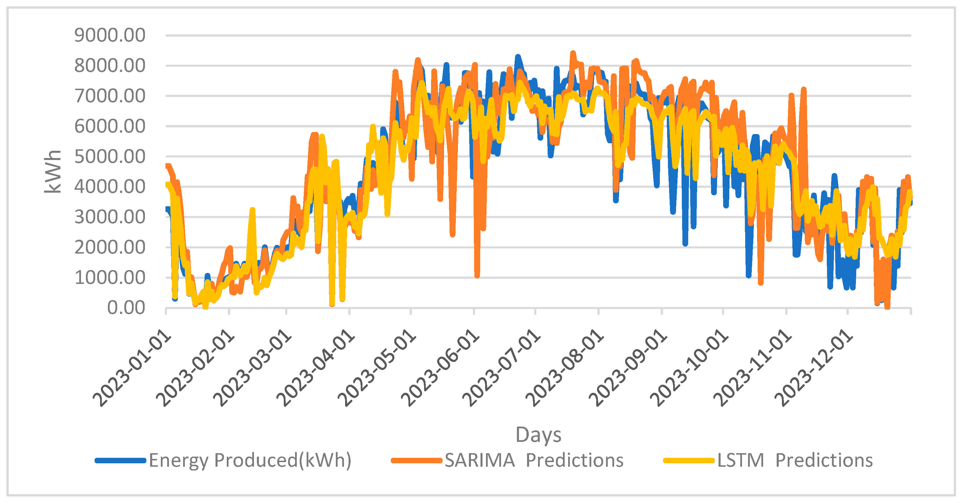
In this study, three different solar energy systems, each with 1MW installed power, were examined. Further, 1-year estimates were made for each system. The data were first implemented in the SARIMA and LSTM models; 70% of each dataset was divided into training, and 30% was divided into testing. The MSE, RMSE, NMSE, MAE, and MAPE methods were used for performance measurements of the prediction results of the models. In Figure 3, Switchboard_A, the energy production, SARIMA, and LSTM prediction results are shown. Forecast results show the results between 1 January 2023 and 31 December 2023.
When Figure 3 is examined, it appears that the LSTM model is more effective than the SARIMA model. In the SARIMA model, there are many sudden rises and falls. In the LSTM model, results closer to energy production are obtained. Table 2 shows the performance results of Plant_A.
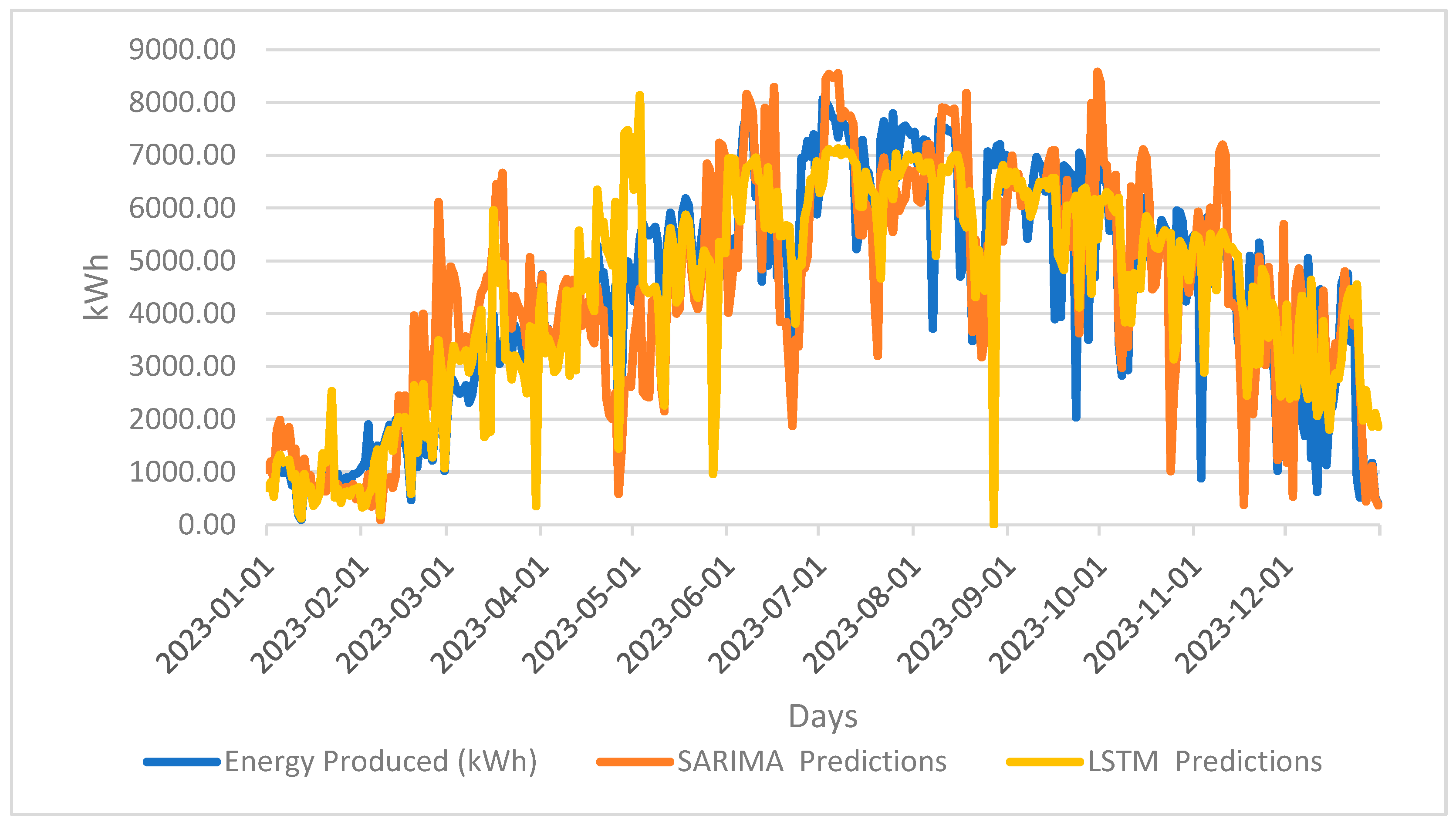
When the performance values of the prediction results are examined, it seems that the LSTM model gives fewer errors. The closer the NMSE results are to zero, the more accurate the results are. Looking at the NMSE results, LSTM showed a better performance with 0.05. Looking at the MAPE results, LSTM showed a higher performance with 81%. The SARIMA model showed a worse result with 61%. In Figure 4, Plant_B, energy production, SARIMA, and LSTM prediction results are shown. Forecast results show the results between 1 January 2023 and 31 December 2023.
When the prediction results of Power Plant_B are examined, the LSTM results yield a better result than the SARIMA model. The prediction results of the LSTM model revealed a result close to the real data. Although there are sudden increases and decreases in a few places, it shows a graph parallel to the actual production data. Table 3 shows the performance results of Plant_B.
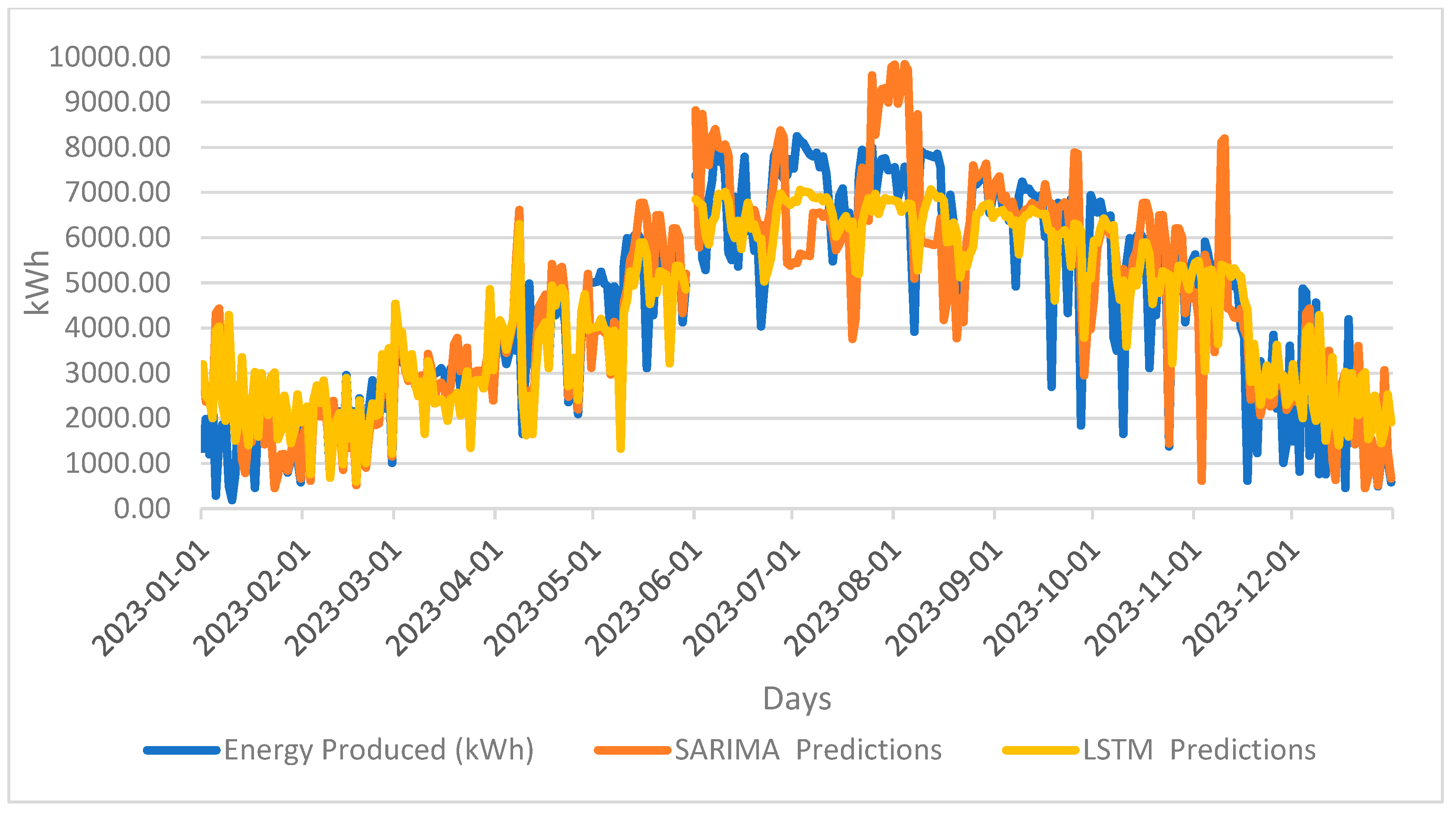
When the performance results are examined, the SARIMA model shows a 49% accuracy rate. The LSTM model performed closer to the real data by 65%. Considering the accuracy rates of the data, LSTM was found to have more realistic data with 0.06. In Figure 5, Switchboard_C, the energy production, SARIMA, and LSTM prediction results are shown. Forecast results show the results between 1 January 2023 and 31 December 2023.
In Plant_C, as in other power plants, the LSTM model appears to be more efficient. There were many sudden rises and falls in the SARIMA model. Sometimes, the difference is huge. Table 4 shows the performance results of Switchboard_C.
A lower accuracy rate was obtained in Santal_C compared to other power plants. An accuracy rate of 59% was determined in the LSTM model. An even lower accuracy rate of 41% was found in the SARMA model. Its accuracy rates remained low compared to other power plants. The highest accuracy rate of the LSTM model was 0.08.
The K-Fold Cross-Validation method divides the dataset into “k” equal parts and creates validation data for each part one by one. Thus, each data point is used as validation data at least once. In this way, the overall performance of the model is evaluated more accurately. In this study, the number k was determined as 5. In other words, the three-year dataset is divided into five. Their distribution is distributed in the same proportions as in the general dataset. Table 5 shows the results after the K-Fold Cross-Validation method.
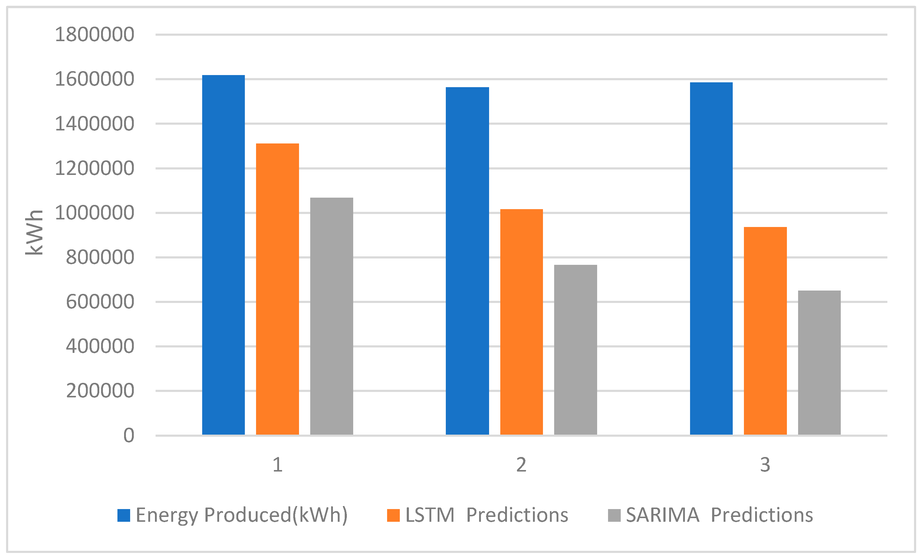
In this study, data from three different solar power plants were used. The installed power of each power plant is the same. They are also close to each other in location. For this reason, there is not much difference in energy production. Figure 6 shows the annual energy production of three different solar power plants, LSTM, and SARIMA models and energy production estimates.
When annual energy production estimates of three different solar power plants were examined, LSTM always showed better results. The LSTM model reached a very high accuracy rate of 81% in the first power plant. The LSTM model reached an accuracy rate of 59% at the third-lowest power plant. As for the SARIMA model, an accuracy rate of 66% was achieved in the first power plant. The highest accuracy rate of the SARIMA model and the lowest accuracy rate of the LSTM model are close to each other. The lowest accuracy rate of the SARIMA model is 41%. This is a very low value.

3.2. Forecasts for Wind Energy System

The CNN-GRU, GRU, LSTM, LSTM-GRU, CNN-LSTM, and CNN-RNN models were used in this study. These models were used in weekly, monthly, and annual forecasts. Table 6 shows the performance of weekly forecasts.
The RMSE value in the CNN-GRU hybrid model is 0.0301, and the closest value to this error value was obtained with the LSTM model. The highest error rate occurred in the independent GRU model. When the results are examined, the values in the error metrics give very similar results to some models. Since these small differences are proportional to the cube of the wind speed in calculating wind power, even the smallest changes in the error metrics obtained are of great importance.
Table 7 presents a comparison of the performances of the CNN-GRU hybrid model and other models. The RMSE value obtained with the CNN-GRU hybrid model is 0.0127, and the closest value to this error value was obtained with the CNN-LSTM model. The highest error rate occurred in the LSTM-GRU model.
The hybrid model proposed in the annual wind speed estimation, which constitutes the last stage of this study, gave more accurate and reliable results. Table 8 presents a comparison of the performances of the proposed hybrid model and other models. The R2 value in the proposed hybrid model is 0.9941, and the regression value closest to this value was obtained in the CNN-LSTM model with 0.9925. The lowest R2 value was calculated with the independent GRU model.
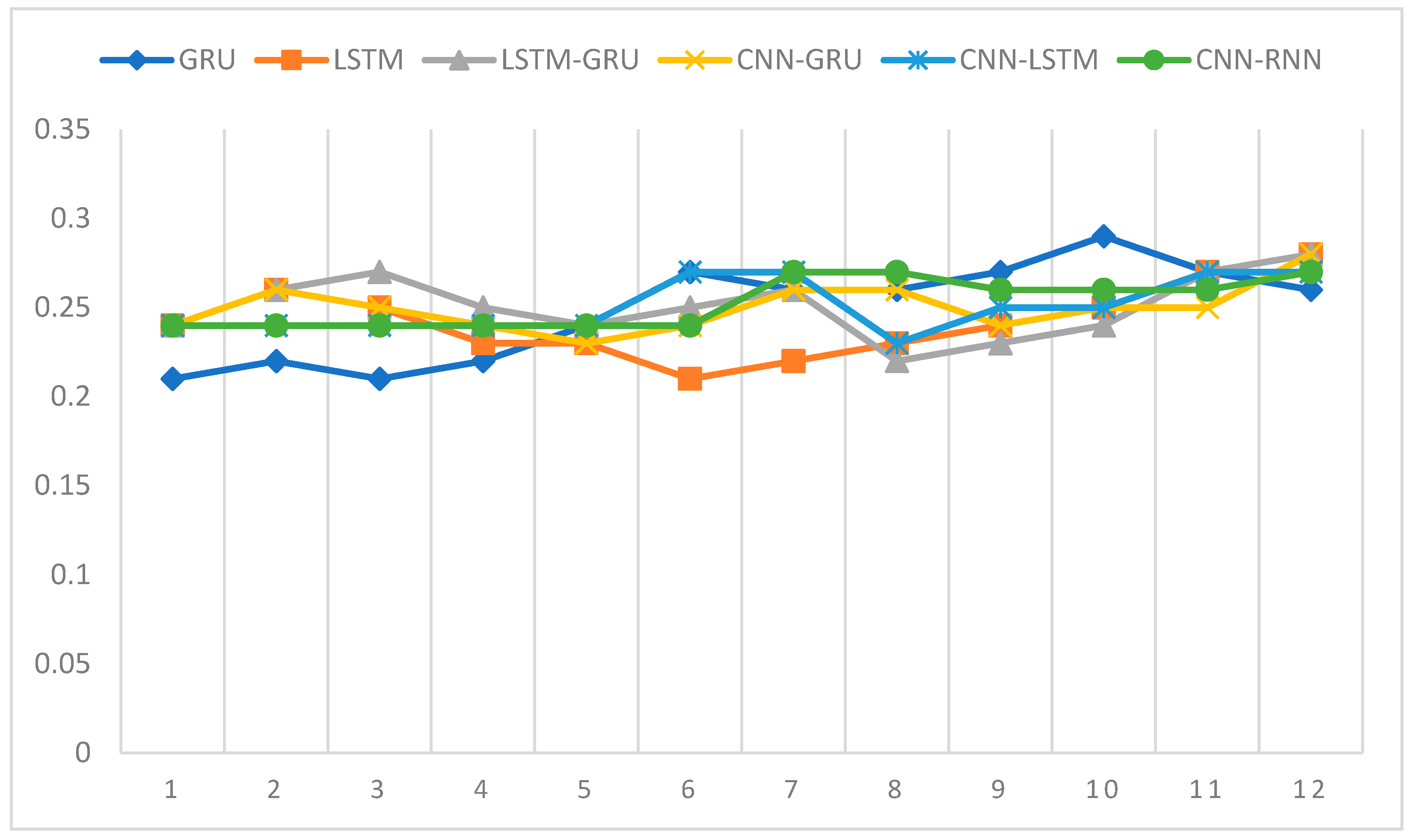
In the second stage of wind energy research, a dataset consisting of 48 weeks was prepared. The change in a 12-week dataset was estimated from this. Figure 7 shows the 12-week evolution of six different deep learning architectures used for the secondary wind energy system.
As a result of this study, when the 12-week data are examined, the results of the deep models used are close to each other. There is variability between the models. For example, while the GRU model gives the worst results in the first week, it gives the best results in the tenth week. Considering the average, the CNN-GRU model performed better than other models.

4. Conclusions

Electricity production estimation was made based on solar power plants. In this study, emphasis was placed on time-series analysis using the deep learning methods LSTM and SARIMA. These methods were applied to three different SPP datasets, and the results were compared using RMSE, MSE, NMSE, MAE, and MAPE, which are frequently used in performance measurements.
Tests of Plant_A, Plant_B, and Plant_C were examined, and realistic results were obtained using both methods. The LSTM results achieved successful values compared to SARIMA. While the LSTM Library used in this study benefited from GPU support, the SARIMA library only benefited from the CPU. Thanks to the computing power of the GPU used in this study, it made positive contributions to obtaining the desired values, both in a short time and consistently.
The wind speed data used in this study were taken at a meteorology station. Three-year data were taken from the meteorological station. Using these data, the error, monthly, and annual estimates were made. In this study, a comparison was made with five different deep learning models in the literature, using CNN-LSTM, CNN-RNN, LSTM-GRU, GRU, LSTM, and CNN-GRU. The performance of the prediction results was evaluated according to MAPE, R2, and RMSE performance criteria. In the results obtained in the weekly wind speed forecasting process, it was observed that the LSTM-GRU model showed more accurate and reliable results. According to the obtained performance criteria, it is clearly seen that the proposed LSTM-GRU model performs better than other models in monthly wind speed forecasts. In the annual wind speed forecasting study, the LSTM-GRU model performed better in terms of forecasting. Looking at the performance criteria results obtained (MAPE: 0.5348, RMSE: 0.1095, and R2: 0.9981), they were determined to have high regression values compared to other models.
In a future study, we will aim to expand and improve the developed model and reduce energy production forecasts to a monthly period. In this way, it can be used to quickly detect problems encountered in the same monthly periods in previous years. Energy production in power plants is handled monthly. Electricity production targets can be achieved by making them according to models. The most appropriate time for maintenance can be determined by making energy production estimates. In this way, time and costs for maintenance can be reduced.
Funding

This research received no external funding

Data Availability Statement

The original contributions presented in the study are included in the article, further inquiries can be directed to the corresponding author.

Conflicts of Interest

The authors declare no conflict of interest.

References

  1. Jiang, P.; Liu, Z.; Niu, X.; Zhang, L. A combined forecasting system based on statistical method, artificial neural networks, and deep learning methods for short-term wind speed forecasting. Energy 2021, 217, 119361. [Google Scholar] [CrossRef]
  2. Kim, H.; Park, M.; Kim, C.W.; Shin, D. Source localization for hazardous material release in an outdoor chemical plant via a combination of LSTM-RNN and CFD simulation. Comput. Chem. Eng. 2019, 125, 476–489. [Google Scholar] [CrossRef]
  3. Cenek, M.; Haro, R.; Sayers, B.; Peng, J. Climate change and power security: Power load prediction for rural electrical microgrids using long short term memory and artificial neural networks. Appl. Sci. 2018, 8, 749. [Google Scholar] [CrossRef]
  4. Lee, D.; Kim, K. Recurrent Neural Network-Based Hourly Prediction of Photovoltaic Power Output Using Meteorological Information. Energies 2019, 12, 215. [Google Scholar] [CrossRef]
  5. Sharadga, H.; Hajimirza, S.; Balog, R.S. Time series forecasting of solar power generation for large-scale photovoltaic plants. Renew. Energy 2020, 150, 797–807. [Google Scholar] [CrossRef]
  6. Wang, Y.; Zou, H.; Chen, X.; Zhang, F.; Chen, J. Adaptive Solar Power Forecasting based on Machine Learning Methods. Appl. Sci. 2018, 8, 2224. [Google Scholar] [CrossRef]
  7. Yildiz, C.; Acikgoz, H.; Korkmaz, D.; Budak, U. An improved residual-based convolutional neural network for very short-term wind power forecasting. Energy Convers. Manag. 2021, 228, 113731. [Google Scholar] [CrossRef]
  8. Li, P.; Zhou, K.; Lu, X.; Yang, S. A hybrid deep learning model for short-term PV power forecasting. Appl. Energy 2020, 259, 114216. [Google Scholar] [CrossRef]
  9. Behera, M.K.; Majumder, I.; Nayak, N. Solar photovoltaic power forecasting using optimized modified extreme learning machine technique. Eng. Sci. Technol. Int. J. 2018, 21, 428–438. [Google Scholar] [CrossRef]
  10. Sun, W.; Wang, A.; Zhang, T. Short-term photovoltaic power interval prediction based on VMD and GOA-KELM algorithms. In Proceedings of the IEEE 4th International Conference on Electronics Technology, Chengdu, China, 7–10 May 2021; pp. 585–590. [Google Scholar]
  11. Mishra, M.; Dash, P.B.; Nayak, J.; Naik, B.; Swain, S.K. Deep learning and wavelet transform integrated approach for short-term solar PV power prediction. Measurement 2020, 166, 108250. [Google Scholar] [CrossRef]
  12. Chandran, V.; Patil, C.K.; Manoharan, A.M.; Ghosh, A.; Sumithra, M.; Karthick, A.; Rahim, R.; Arun, K. Wind power forecasting based on time series model using deep machine learning algorithms. Mater. Today Proc. 2021, 47, 115–126. [Google Scholar] [CrossRef]
  13. Ding, M.; Zhou, H.; Xie, H.; Wu, M.; Liu, K.-Z.; Nakanishi, Y.; Yokoyama, R. A time series model based on hybrid-kernel least-squares support vector machine for short-term wind power forecasting. ISA Trans. 2021, 108, 58–68. [Google Scholar] [CrossRef]
  14. Gao, B.; Huang, X.; Shi, J.; Tai, Y.; Zhang, J. Hourly forecasting of solar irradiance based on CEEMDAN and multi-strategy CNN-LSTM neural networks. Renew. Energy 2020, 162, 1665–1683. [Google Scholar] [CrossRef]
  15. Greff, K.; Srivastava, R.K.; Koutník, J.; Steunebrink, B.R.; ve Schmidhuber, J. LSTM: A search space odyssey. IEEE Trans. Neural Netw. Learn. Syst. 2016, 28, 2222–2232. [Google Scholar] [CrossRef]
  16. Zheng, L.; Lu, W.; Zhou, Q. Weather image-based short-term dense wind speed forecast with a ConvLSTM-LSTM deep learning model. Build. Environ. 2023, 239, 110446. [Google Scholar] [CrossRef]
  17. Zhang, D.; Hu, G.; Song, J.; Gao, H.; Ren, H.; Chen, W. A novel spatio-temporal wind speed forecasting method based on the microscale meteorological model and a hybrid deep learning model. Energy 2023, 288, 129823. [Google Scholar] [CrossRef]
  18. Chen, H.; Zhang, Q.; Birkelund, Y. Machine learning forecast of Scandinavian numerical weather prediction wind model residuals with control theory for wind energy. Energy Rep. 2022, 8 (Suppl. 13), 661–668. [Google Scholar] [CrossRef]
  19. Tan, M. İkincil Ayrıştırma Tekniği Kullanarak Yapay Sinir Ağı Temelli Çok Adımlı Rüzgar Hızı Tahmini. Master’s Thesis, Tokat Gaziosmanpaşa Üniversitesi, Elektrik Elektronik Mühendisliği Anabilim Dalı, Tokat, Türkiye, 2020. [Google Scholar]
  20. Görgel, P.; ve Kavlak, E. Uzun kısa süreli hafıza ve evrişimsel sinir ağları ile rüzgar enerjisi üretim tahmini. Dicle Üniversitesi Mühendislik Fakültesi Mühendislik Derg. 2020, 11, 69–80. [Google Scholar] [CrossRef]
  21. Livieris, I.E.; Pintelas, E.; Pintelas, P. A CNN–LSTM model for gold price time-series forecasting. Neural Comput. Appl. 2020, 32, 17351–17360. [Google Scholar] [CrossRef]
  22. Xiong, J.; Peng, T.; Tao, Z.; Zhang, C.; Song, S.; Nazir, M.S. A dual-scale deep learning model based on ELM-BiLSTM and improved reptile search algorithm for wind power prediction. Energy 2023, 266, 126419. [Google Scholar] [CrossRef]
  23. Yaghoubirad, M.; Azizi, N.; Farajollahi, M.; Ahmadi, A. Deep learning-based multistep ahead wind speed and power generation forecasting using direct method. Energy Convers. Manag. 2023, 281, 116760. [Google Scholar] [CrossRef]
  24. Azad, H.B.; Mekhilef, S.; Ganapathy, V.G. Long-Term Wind Speed Forecasting and General Pattern Recognition Using Neural Networks. IEEE Trans. Sustain. Energy 2014, 5, 546–553. [Google Scholar] [CrossRef]
  25. Tascikaraoglu, A.; Sanandaji, B.M.; Poolla, K.; Varaiya, P. Exploiting sparsity of interconnections in spatio-temporal wind speed forecasting using Wavelet Transform. Appl. Energy 2015, 165, 735–747. [Google Scholar] [CrossRef]
  26. Zhen, Z.; Qiu, G.; Mei, S.; Wang, F.; Zhang, X.; Yin, R.; Li, Y.; Osório, G.J.; Shafie-Khah, M.; Catalão, J.P. An ultra-short-term wind speed forecasting model based on time scale recognition and dynamic adaptive modeling. Int. J. Electr. Power Energy Syst. 2021, 135, 107502. [Google Scholar] [CrossRef]
  27. Gu, Y.; Xu, W.; Tang, D.; Yuan, Y.; Chai, Z.; Ke, Y.; Guerrero, J.M. A Combined Wind Forecasting Model Based on SSA and WNN: Application on Real Case of Ningbo Zhoushan Port. J. Mar. Sci. Eng. 2023, 11, 1636. [Google Scholar] [CrossRef]
  28. Tang, D.; Fang, Y.P.; Zio, E. Vulnerability analysis of demand-response with renewable energy integration in smart grids to cyber attacks and online detection methods. Reliab. Eng. Syst. Saf. 2023, 235, 109212. [Google Scholar] [CrossRef]
  29. Liu, H.; Mi, X.; Li, Y.; Duan, Z.; Xu, Y. Smart wind speed deep learning based multi-step forecasting model using singular spectrum analysis, convolutional Gated Recurrent Unit network and Support Vector Regression. Renew. Energy 2019, 143, 842–854. [Google Scholar] [CrossRef]
  30. Chatuverdi, S.; Rajasekar, E.; Natarajan, S.; McCullen, N. A Comparative assessment of SARIMA, LSTM RNN and Fb Prophet models to forecast total and peak monthly energy demand for India. Energy Policy 2022, 168, 113097. [Google Scholar]
  31. Akaike, H. A new look at the statistical model identification. IEEE Trans. Autom. Control 1974, 19, 716–723. [Google Scholar] [CrossRef]
  32. Dickey, D.A.; Fuller, W.A. Distribution of the estimators for autoregressive time series with a unit root. J. Am. Stat. Assoc. 1979, 74, 427–431. [Google Scholar]
  33. Ghofrani, M.; Alolayan, M. Time series and renewable energy forecasting. Time Ser. Anal. Appl. 2018, 10, 77–92. [Google Scholar]
  34. Xu, P.; Zhang, M.; Chen, Z.; Wang, B.; Cheng, C.; Liu, R. A Deep Learning Framework for Day Ahead Wind Power Short-Term Prediction. Appl. Sci. 2023, 13, 4042. [Google Scholar] [CrossRef]
Figure 1. LSTM and SARIMA basic flow diagram of this study.
Energies 17 04031 g001
Figure 2. Locations of solar energy systems and wind energy systems used for this study.
Energies 17 04031 g002
Figure 3. Forecast results for Power Plant_A.
Energies 17 04031 g003
Figure 4. Prediction results for Power Plant_B.
Energies 17 04031 g004
Figure 5. Prediction results for Plant_C.
Energies 17 04031 g005
Figure 6. Annual energy production of three different solar power plants and energy production predictions with LSTM and SARIMA models.
Energies 17 04031 g006
Figure 7. Twelve-week evolution across six different deep learning architectures.
Energies 17 04031 g007
Table 1. The general structure of the LSTM model.
LayerOutput SizeNumber of Parameters
LSTM324864
Dropout320
LSTM_1255800
Dense126
Table 2. Performance results of Plant_A.
ModelRMSEMSENMSEMAEMAPE
SARIMA1481.452,459,6320.081265.9666%
LSTM1087.951,526,9140.05856.1281%
Table 3. Performance results of Plant_B.
ModelRMSEMSENMSEMAEMAPE
SARIMA1895.153,859,2580.121525.5149%
LSTM1426.881,782,2010.071048.4165%
Table 4. Performance results of Plant_C.
ModelRMSEMSENMSEMAEMAPE
SARIMA1805.123,105,5280.151305.2141%
LSTM1294.121,748,1020.081047.4459%
Table 5. The results after the K-Fold Cross-Validation method.
Power PlantModelk1k2k3k4k5% Average
ALSTM79.7881.4982.0181.4781.3281.21
SARIMA64.2565.8767.5867.1565.7866.13
BLSTM65.2565.1565.8165.3265.1965.34
SARIMA51.0751.1949.7848.4749.2549.95
CLSTM61.3558.9860.7160.3257.0759.69
SARIMA68.4265.2866.6866.366.3866.61
Table 6. Weekly forecast performance comparison.
MetricGRULSTMLSTM-GRUCNN-GRUCNN-LSTMCNN-RNN
MAPE0.2410.10480.13250.11490.12440.1815
R20.92480.9910.97480.98910.9810.9688
RMSE0.06470.03120.0380.03020.03490.0471
Table 7. Monthly forecast performance comparison.
MetricGRULSTMLSTM-GRUCNN-GRUCNN-LSTMCNN-RNN
MAPE0.37990.34180.35000.04150.04710.05150
R20.08150.085550.79440.99410.99250.9981
RMSE0.10790.089210.11480.01190.01250.21896
Table 8. Annual forecasting performance benchmark.
MetricGRULSTMLSTM-GRUCNN-GRUCNN-LSTMCNN-RNN
MAPE1.1471.0891.0140.53480.85140.7736
R20.4810.76880.75120.99810.99250.9928
RMSE0.15480.10950.106250.02180.02150.0239
Disclaimer/Publisher’s Note: The statements, opinions and data contained in all publications are solely those of the individual author(s) and contributor(s) and not of MDPI and/or the editor(s). MDPI and/or the editor(s) disclaim responsibility for any injury to people or property resulting from any ideas, methods, instructions or products referred to in the content.