Article

A Parallel Prediction Model for Photovoltaic Power Using Multi-Level Attention and Similar Day Clustering

by
Jinming Gao
1,
Xianlong Su
1,
Changsu Kim
1,
Kerang Cao
2 and
Hoekyung Jung
1,*
1
Department of Computer Science and Engineering, Pai Chai University, 155-40 Baejae-ro, Daejeon 35345, Republic of Korea
2
Department of Computer Science and Engineering, Shenyang University of Chemical Technology, Shenyang 110142, China
*
Author to whom correspondence should be addressed.
Energies 2024, 17(16), 3958; https://doi.org/10.3390/en17163958
Submission received: 25 June 2024 / Revised: 31 July 2024 / Accepted: 8 August 2024 / Published: 9 August 2024
(This article belongs to the Section F5: Artificial Intelligence and Smart Energy)

Abstract

:
Photovoltaic (PV) power generation is significantly impacted by environmental factors that exhibit substantial uncertainty and volatility, posing a critical challenge for accurate PV power prediction in power system management. To address this, a parallel model is proposed for PV short-term prediction utilizing a multi-level attention mechanism. Firstly, gray relation analysis (GRA) and an improved ISODATA algorithm are used to select a dataset of similar days with comparable meteorological characteristics to the forecast day. A transformer encoder layer with multi-head attention is then used to extract long-term dependency features. Concurrently, BiGRU, optimized with a Global Attention network, is used to capture global temporal features. Feature fusion is performed using Cross Attention, calculating attention weights to emphasize significant features and enhancing feature integration. Finally, high-precision predictions are achieved through a fully connected layer. Utilizing historical PV power generation data to predict power output under various weather conditions, the proposed model demonstrates superior performance across all three climate types compared to other models, achieving more reliable predictions.

Graphical Abstract

1. Introduction

The emergence of low-carbon clean power systems has brought sustainable energy generation to the forefront of global interest [1]. Photovoltaic (PV) technology plays a crucial role in these new power systems. However, it is susceptible to meteorological conditions [2], which exhibit complex and fluctuating features and structures [3]. Therefore, to guarantee the secure, consistent, and cost-effective functioning of power systems, accurate prediction of PV power generation is essential to fulfill the demands of power system planning, operation, control, and scheduling [4].
Various prediction methods have been identified for PV power prediction, including mathematical–physical modeling, statistical time series, and machine learning methods [5]. The mathematical–physical modeling approach involves simplifying the output power calculation based on the physical structure of the PV power generation system through mathematical modeling, rather than relying on weather and other numerical values [6,7]. While this method offers a simple calculation process, it fails to replicate the fluctuations observed in actual operation, resulting in a lower prediction accuracy. Statistical time series methods utilize statistical models that build upon mathematical and physical models to forecast PV power output. Commonly employed statistical prediction techniques include the AutoRegressive Integrated Moving Average (ARIMA) method [8], the AutoRegressive and Moving Average (ARMA) method [9], and regression analysis [10]. These methods are effective for short-term linear time series predictions; however, their efficiency diminishes with longer prediction horizons or when faced with nonlinear challenges. Recent developments in intelligent sensing and communication technologies have facilitated the collection of vast amounts of data, such as load, weather, and geographical information. These data serve as a crucial foundation for artificial intelligence, big data analytics, and other methodologies in PV power prediction. Consequently, machine learning methods, known for their capacity to extract complex abstract features, are gaining significant attention due to their learning capabilities [11].
Machine-learning-based prediction methods can be categorized into shallow and deep learning models. Deep learning models are known to be more effective in capturing data features and patterns compared to shallow learning models [12]. They are commonly utilized in the analysis and processing of large-scale data, such as in PV prediction [13,14,15]. Rodríguez et al. [16] employed feed-forward neural networks in conjunction with spatiotemporal parameters to improve the accuracy of short-term predictions. Annalisa et al. [17] utilized a Nonlinear AutoRegressive with eXogenous inputs (NARX) network for PV prediction, which can handle nonlinear relationships and consider external input impacts, and it exhibits superior flexibility and performance compared to traditional feedforward networks. As machine learning technology advances, various hybrid models have been introduced to address the limitations of individual models and produce more accurate predictions. This has led to the development of diverse prediction combinations. Agga et al. [18] proposed a hybrid prediction method that combines a Convolutional Neural Network (CNN) with a Long Short-Term Memory (LSTM) model, resulting in improved prediction accuracy. Tang et al. [19] integrated the attention mechanism with CNN and Bidirectional Long Short-Term Memory (BiLSTM) to create a day-ahead PV prediction model. This model effectively examines the causal relationship between features and outputs through the attention mechanism, outperforming single machine learning models in terms of prediction accuracy. These studies demonstrate that combined prediction models generally yield superior prediction results compared to individual prediction models.
The results of the aforementioned model investigations exhibit suboptimal performance in forecasting long time series. This limitation predominantly stems from the incapacity of networks such as CNN and LSTM to sustain extended sequences and adequately capture long-term dependencies [20]. Transformer models integrate the attention mechanism to augment their capability of capturing long-term dependencies [21]. However, in situations with restricted computational resources and limited datasets, this strategy may become unstable, potentially resulting in information loss. To address this issue, Kim et al. [22] combined the Transformer model with LSTM, leveraging the strengths of both models to improve local and global feature extraction and improve prediction accuracy. Moon et al. [23] merged the Transformer model with CNN, offering precise, immediate forecasts and the capacity to discern long-term power generation trends. In addition to improvements in composite models, the temporal modeling and optimization of long series can be achieved by modifying the Transformer model’s structure or introducing new iterations of the attention mechanism, such as informer [24], autoformer [25], and crossformer [26]. These variations in time series prediction have demonstrated positive results, albeit with increased structural complexity.
The current focus of research on PV power prediction primarily emphasizes enhancing model accuracy, often neglecting the quality of the training dataset and the impact of various feature factors on the output. To bridge this research gap, this study integrates the strengths of multiple models and devises a deep learning framework that integrates similar day selection, data feature selection, and a multi-level attention mechanism for PV power prediction. This approach leverages the advantages of each module without significantly escalating the overall complexity. The training dataset is refined through gray relation analysis (GRA) and an improved ISODATA clustering algorithm to identify a dataset comprising days with akin meteorological characteristics to the forecast day. Furthermore, weather conditions are classified into different categories, such as sunny, cloudy, and rainy days, across different seasons to reduce the data needed for prediction. Long-term dependency features are extracted utilizing a Transformer encoder layer with multi-attention, while global temporal features are captured by a BiGRU network optimized with Global Attention. Feature fusion is facilitated through Cross Attention, enabling the model to concentrate on crucial features by computing attention weights, thereby enhancing feature integration. Ultimately, precise predictions are generated using a fully connected layer.
This paper integrates the strengths of multiple models to develop a short-term PV power prediction model that incorporates similar day selection, data processing, attention mechanisms, and deep learning. This approach effectively addresses the limitations of individual models in terms of long-term data dependence and global feature extraction. The main innovations of this paper are outlined as follows:
(1)
Improved Clustering and Data Quality: Employing similar day selection and an improved ISODATA clustering algorithm improves the clustering impact, categorizing the dataset by different seasons and climate types. This approach reduces the amount of data required for prediction and improves data quality.
(2)
Transformer Encoder Layer: Dependencies between different positions in the sequence are extracted and global contextual information is captured using a Transformer encoder layer with a multi-head attention mechanism. Additionally, a parallel structure is implemented to accelerate model training and inference.
(3)
BiGRU with Global Attention: A BiGRU network, optimized with Global Attention, captures global temporal features, enhancing the model’s ability to perceive time-domain characteristics of multi-feature sequences.
(4)
Cross Attention for Feature Fusion: Cross Attention is employed to fuse information from different sources, enhancing the representation capability of features and achieving high-accuracy predictions.

2. Meteorological Data Processing

2.1. Data Preprocessing

Historical data form the foundation of prediction, and to ensure accuracy, the data must undergo preprocessing to improve their quality. The preprocessing steps are summarized as follows:
(1)
It must be ensured that data recording intervals, feature labels, and timestamps are uniformly formatted;
(2)
For noncontinuous missing data, interpolation methods can be used for estimation. Given the strong periodicity of load data, the Lagrangian interpolation method is employed to estimate missing values and fill in the gaps [27];
(3)
Evident errors and repeatability issues, such as sudden zero values or extremely high values exceeding system capacity, should be identified and corrected. Invalid data must be discarded or replaced, as PV systems are expected to operate normally with slow, gradual changes in power. Invalid data points can be replaced by the average value of the preceding and succeeding time points.

2.2. Similar Day Selection

The performance of PV power generation systems is impacted not only by their structural aspects but also by various weather conditions. Predicting PV power generation is complex due to the impact of numerous non-critical factors, which can reduce the prediction accuracy. This study collected meteorological data such as total horizontal irradiance, scattered horizontal irradiance, temperature, relative humidity, wind speed, and wind direction. Pearson’s coefficient was utilized to identify meteorological factors that have a higher correlation with power generation. These factors were then used to select similar days [28], aiming to eliminate the impact of less significant meteorological data on the selection process. The calculation is presented as follows:
ρ x y = i = 1 n X i X ¯ Y i Y ¯ i = 1 n X i X ¯ 2 i = 1 n Y i Y ¯ 2
where n denotes the total number of samples; X i denotes the meteorological parameter at time i; X ¯ denotes the average value of the meteorological parameter; Y i denotes the PV output power at time i; and Y ¯ denotes the average value of the PV output power. The correlation coefficients between each meteorological factor and the PV power were calculated and are outlined in Table 1. The analysis revealed that irradiance, temperature, humidity, and wind speed exhibited the highest Pearson correlation coefficients with power generation, suggesting a strong correlation. Therefore, these four variables were selected for the calculation of similar days.
Irradiance has a direct impact on the power generation efficiency of PV panels, while temperature impacts the conversion efficiency of PV panels, and wind speed and humidity are significant factors impacting the heat dissipation of the system [29]. As a result, this study chose weather variables such as irradiance, temperature, wind speed, and humidity as the input vectors for prediction. This selection aimed to simplify the data complexity and improve the prediction accuracy.
However, the accuracy of power prediction for a given day can be impacted by various weather conditions. Due to the inherent variability in weather patterns, relying only on the proximity of the day for training prediction models may introduce a certain level of error. To improve the prediction accuracy, the gray correlation analysis method is employed to filter the data pertaining to different meteorological factors. This method involves calculating the gray correlation value for each sample to elucidate the relationships among meteorological variables and to evaluate their similarities. In this research, data from days exhibiting a gray correlation value exceeding 0.8 with the prediction day data were selected as the training dataset [30].
(1)
Meteorological feature vectors are developed based on the selected meteorological features M:
M = R ¯ , T ¯ , W ¯ , H ¯
where R ¯ denotes the average daily irradiance; T ¯ denotes the average daily temperature; W ¯ denotes the average daily wind speed; and H ¯ denotes the average daily humidity.
(2)
After processing each component, the meteorological feature vectors for the forecast day and d day are x 0 and x d , respectively.
x 0 = x 01 , x 02 , x 03 , x 04
x d = x d 1 , x d 2 , x d 3 , x d 4
(3)
The correlation coefficients of x 0 and x d in the s (s = 1, 2, …, 4) classification, ξ d s , are determined as follows:
ξ d s = a + r b x 0 s x d s + r b
a = min d min s x 0 s x d s
b = max d max s x 0 s x d s
where r denotes the resolution coefficient, which takes a value between [0,1]. In this study, r = 0.5.
(4)
The correlation coefficient of each component is synthesized, and the similarity between x 0 and x d is defined as γ x 0 , x d .
γ x 0 , x d = 1 m s = 1 4 ξ d s
where m denotes the total number of components of the meteorological eigenvectors.

2.3. Improved ISODATA Clustering Algorithm

The process yields a rough set of days with similar PV prediction, which can be further refined through clustering techniques to improve dataset optimization [31]. This study focuses on applying clustering methods to meteorological data to improve the prediction accuracy by minimizing intra-category variances and maximizing inter-category differences. Commonly used clustering algorithms such as K-means and ISODATA [32] are employed. While the K-means algorithm is valued for its simplicity and efficiency, challenges arise in determining the optimal k value and initial clustering centers. Furthermore, its reliance on Euclidean distance metrics may not adequately capture temporal changes in high-dimensional features, particularly in load forecasting for different time periods. The ISODATA algorithm addresses these limitations by incorporating merging and splitting operations to dynamically adjust cluster numbers based on cluster characteristics. However, the random selection of initial cluster centers may lead to slow convergence and unpredictable results. Additionally, the continued use of Euclidean distance metrics may limit its ability to capture high-dimensional features effectively. To address these issues, this paper introduces an improved ISODATA algorithm that optimizes the configuration of initial clustering centers and Euclidean distances.

2.3.1. Optimization of Initial Clustering Centers

The fundamental concept of this optimization approach is to improve the separation between initial clustering centers during their selection process. Initially, the selection of the first clustering center is random. Subsequent clustering centers are selected based on their distance from the already selected centers, with points that are farther away from the existing centers being more likely to be selected.
This optimization technique is designed to mitigate the issue of initial clustering centers being in close proximity. When the initial centers are too close, there is a risk of them being grouped into the same cluster, which would require additional iterations to separate them into different clusters. Conversely, widely dispersed initial centers are more likely to correspond to separate clusters, facilitating quicker convergence and yielding improved clustering results.
The steps in the optimization algorithm for initial clustering center selection are given as follows:
(1)
A random sample from the dataset is selected to serve as the first initial clustering center.
(2)
For each remaining sample xi, its distance from each existing clustering center is calculated, and the shortest distance d(xi), is recorded.
(3)
The probability of each sample xi being selected as the next clustering center is proportional to d x i 2 x D d x i 2 . Samples with larger d(xi) have a higher probability of being selected.
(4)
Step 2 is repeated until k initial clustering centers are selected.
This strategy ensures that the selected initial clustering centers are widely separated, thereby enhancing the probability of them belonging to different clusters and expediting the convergence process.

2.3.2. Kernel Method

The optimization of Euclidean spatial distance is achieved through the utilization of a kernel method. Initially, the data from the original space undergo mapping to a high-dimensional feature space via nonlinear mapping, followed by clustering. This mapping improves the probability of linear separability among data points. In the high-dimensional space, the clustering algorithm computes distances between samples based on the high-dimensional features of the load curves, leading to improved clustering performance. However, computations in the high-dimensional space are complex. To mitigate this issue, the kernel function K(x,z) is introduced.
Let X denote the input space and H denote a higher-dimensional space. Let ϕ(x) be a mapping function that maps a point x in space X to a point h in space H, such that h = ϕ(x). If there is a function K(x,z) for all x,zX, such that K(x,z) = ϕ(xϕ(z), then the inner product of the mappings of two points can be directly computed in the original space X using the kernel function.
The distance between two samples is typically represented by a kernel function in clustering calculations as follows:
d ( x i , x j ) = ϕ ( x i ) ϕ ( x j ) 2 = ϕ ( x i ) 2 2 ϕ ( x i ) ϕ ( x j ) + ϕ ( x j ) 2 = K ( x i , x j ) 2 K ( x i , x j ) + K ( x i , x j )
This is calculated as the distance from each sample xi to each clustering center μj. In the high-dimensional space, the distance is determined as follows:
d ( x i , μ j ) = ϕ ( x i ) ϕ ( μ j ) 2 = ϕ ( x i ) 2 2 ϕ ( x i ) ϕ ( μ j ) + ϕ ( μ j ) 2
The center of clustering in the high-dimensional space can be expressed as follows:
ϕ ( μ j ) = 1 C j ϕ ( x ) C j ϕ ( x )
By substituting Equation (11) into Equation (10), the distance between sample xi and clustering center μj can be further solved as follows:
d ( x i , μ j ) = ϕ ( x i ) 2 2 C j ϕ ( x ) C j ϕ ( x i ) ϕ ( x ) + 1 C j 2 ϕ ( x 1 ) C j ϕ ( x 2 ) C j ϕ ( x 1 ) ϕ ( x 2 ) = K ( x i , x i ) 2 C j ϕ ( x ) C j K ( x i , x ) + 1 C j 2 ϕ ( x 1 ) C j ϕ ( x 2 ) C j K ( x 1 , x 2 )
The equation above illustrates that the approach has the capability to bypass the mapping function and perform calculations only based on the kernel function. In this study, the Gaussian kernel function is employed as K ( x , z ) = exp ( γ x z 2 ) .

2.3.3. Evaluation Criteria

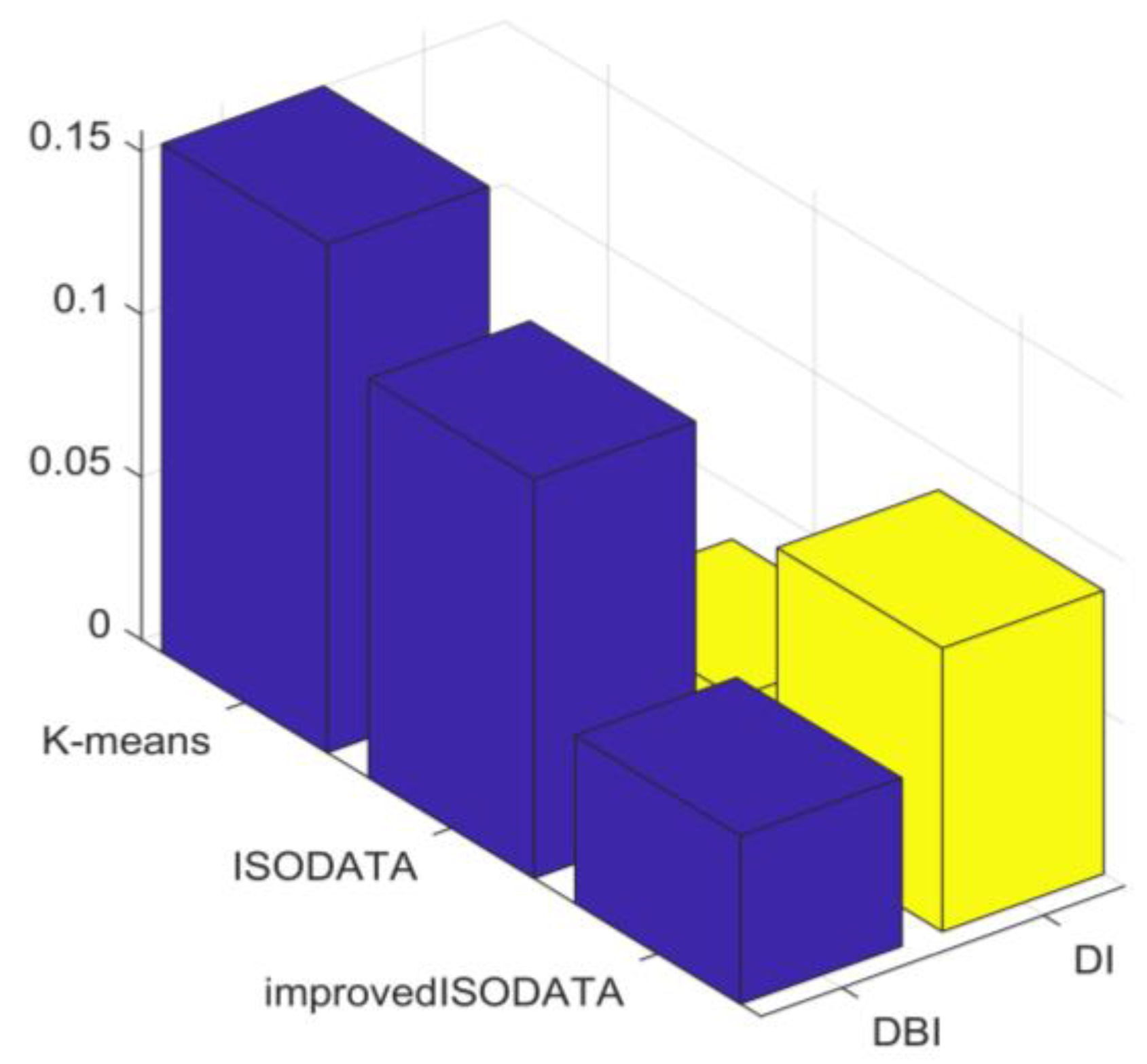
A desirable clustering result is defined by a high level of similarity within clusters and a low level of similarity between clusters. To assess clustering effectiveness based on this principle, this study employs the Davies–Bouldin Index (DBI) and Dunn Index (DI) [33].
D B I = 1 k i = 1 k max j = 1 , , k , j i ( a ν g ( C i ) + a ν g ( C j ) d c e n ( μ i , μ j ) )
D I = min 1 i k { min j = 1 , , k , j i ( d min ( C i , C j ) max 1 l k d i a m ( C l ) ) }
Let C denote the clustering result, dist(xi,xj) denote the distance between two samples, avg(C) denote the average distance between samples within a cluster, diam(C) denote the maximum distance between samples within a cluster, dmin(Ci,Cj) denote the minimum distance between samples in clusters Ci and Cj, and dcen(Ci,Cj) denote the distance between the centers of clusters Ci and Cj.
The expressions of DBI and DI are examined as follows: a smaller avg(C) suggests greater similarity within clusters, while a larger dcen(Ci,Cj) indicates lower similarity between clusters. Therefore, a lower DBI value is more desirable, as it signifies higher intra-cluster similarity and lower inter-cluster similarity. Conversely, a larger dmin(Ci,Cj) implies lower inter-cluster similarity, and a smaller diam(C) indicates higher intra-cluster similarity. Therefore, a higher DI value is preferable, as it indicates lower similarity between clusters and higher similarity within clusters.

3. Multi-Level Attention Parallel Prediction Model

3.1. Transformer–Multi-Head Attention

The data intended for loading demonstrates significant nonlinearity, time-varying characteristics, and complex seasonal periodicity. Conventional load forecasting models are insufficient in capturing these complex features effectively. Consequently, a sampling method has been devised to mirror the structure of the Transformer encoder, leveraging the multi-attention mechanism. This method capitalizes on the Transformer model’s exceptional ability to acquire remote dependencies, enabling the capture of complex external features and nonlinear relationships within PV data. By integrating these aspects into the prediction model, the accuracy of the predictions is improved. In Domhan et al. [34], the primary component within the Transformer model is the encoder layer. To streamline the model, this study focuses only on the encoder layer’s structure, which comprises the multi-head attention mechanism and feed-forward neural network. The configuration of the Transformer encoder structure is illustrated in Figure 1.
Self-attention is a mechanism that modulates the importance of individual features in the output by evaluating the relevance of features within the input sequence. The multi-attention approach amplifies the model’s capacity for representation by conducting several self-attention operations concurrently, enabling the capture of diverse characteristics of the sequence data across different subspaces.
The multi-head attention mechanism update equation can be expressed as follows:
Attention ( Q , K , V ) = softmax Q K T d k V head i = Attention ( Q i , K i , V i ) , i = 1 , , n MultiHead ( Q , K , V ) = Concat ( head 1 , , head n ) W O
where Q, K, and V denote the query, key, and value matrices, respectively; dk denotes the dimension of the key vector; and WO denotes the linear transformation matrix that transforms the result of the attention computation.
Subsequently, the attention mechanism extracts features that undergo additional extraction and transformation through a feed-forward neural network. This integration of feature information from diverse sources amplifies the model’s nonlinear and expressive capabilities. The equation can be expressed as follows:
FFN ( x ) = max ( 0 , x W 1 + b 1 ) W 2 + b 2
To address the issue of gradient vanishing in the training process, a residual connection is implemented, where the output of each sublayer is added to its input. Additionally, layer normalization is incorporated to improve the stability of the training procedure.

3.2. BiGRU-Global Attention

The transformer model demonstrates improved performance in extracting information from long sequences; however, it may sacrifice many local extraction details. For PV power-related time data, there exists a bidirectional flow of information that encompasses both forward and backward temporal relationships. To delve deeper into the temporal dynamics among PV power sequences, this research leveraged the BiGRU model for PV power prediction. The BiGRU model amalgamates the strengths of GRU and bidirectional Recurrent Neural Networks (RNNs), enabling the utilization of past and future sequence information for model training [35]. This model exhibits superior nonlinear expression capabilities and improves prediction accuracy for time series data by effectively incorporating both preceding and succeeding information.
The structure of the BiGRU model (Figure 2) comprises the input, forward propagation, back propagation, and output layers. The forward and back propagations offer the historical and future time correlation information of the input PV data sequence, respectively. The detailed configuration is outlined as follows:
forward   GRU :   h t = GRU ( x t , h t 1 )
backward   GRU :   h t = GRU ( x t , h t + 1 )
output :   h t = [ h t ; h t ]
where xt denotes the tth element of the input sequence; h t and h t denote the hidden states of the forward and backward GRUs, respectively; and ht denotes the output of BiGRU.
The BiGRU structure demonstrates effectiveness in capturing short-term dependencies, but it may prove insufficient for long-range dependencies. The incorporation of the Global Attention mechanism [36] enables the model to adaptively modulate its reliance on global information at every time step via the attention weight matrix, thereby enhancing its ability to capture long-range dependencies and complex patterns within the load data. The Global Attention framework is depicted in Figure 3.
Global Attention initially computes the correlation between each time step based on Equations (20) and (21), utilizing the BiGRU output. It dynamically modifies the weights of each time step, facilitating the model to amalgamate global information in the prediction.
e t j = score ( h t , h j )
α t j = exp ( e t j ) k = 1 T exp ( e t k )
Subsequently, the context vector is calculated using Equation (22) to incorporate global information into the prediction of the current time step, thereby resulting in the final output yt.
c t = j = 1 T α t j h j
y t = tanh ( W [ c t ; h t ] + b )
The incorporation of the Global Attention mechanism enables the utilization of global contextual information in load forecasting, particularly for PV data. Additionally, it allows for the adjustment of the impact of each time step based on the input data characteristics. This improvement increases the model’s flexibility and adaptability, thereby improving its efficiency in addressing the distinctive attributes inherent in PV data.

3.3. Cross Attention

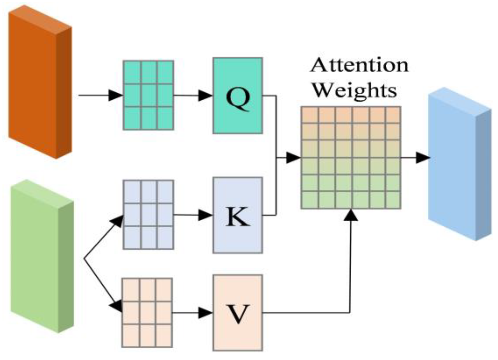
The Cross Attention mechanism integrates the outputs of various models (Transformer and BiGRU–Global Attention) [37], allowing the model to leverage multiple features concurrently. This improves the feature representation of the model, enabling it to capture more complex patterns of PV power variations. Additionally, the Cross Attention mechanism facilitates the model in dynamically regulating the significance of different features, thereby enhancing the adaptability and resilience of the model across various PV power scenarios. The structure of the Cross Attention mechanism is illustrated in Figure 4.
The Cross Attention equation is expressed as follows:
CrossAttention ( Q , K , V ) = softmax Q K T d k V
where Q denotes the output of one module, while K and V denote the output of another module. The results of Equation (25) for Transformer and Equation (26) for BiGRU–Global Attention are combined in the Cross Attention Equation (27) to yield Equations (28) and (29). Subsequently, the ultimate output Hfusion is obtained through fusion.
H T = Transformer ( X )
H B = BiGRUGlobal ( X )
H T B = CrossAttention ( H T , H B , H B )
H B T = CrossAttention ( H B , H T , H T )
H f u s i o n = Concat ( H T B , H B T )
Finally, Cross Attention features are utilized in conjunction with the average pooling layer to reshape the tensor, ultimately generating the final prediction through the fully connected layer.

3.4. Framework of This Paper

Combining the benefits of various models, a multi-level attention parallel prediction model was developed. This model leverages a parallel structure to predict targets at multiple time steps concurrently, ensuring accuracy, and accelerating the training and inference processes. The proposed model improves the extraction of long-term dependencies and improves the perception of temporal features in multi-feature sequences, leading to increased accuracy and reduced computational complexity compared to traditional ensemble models and Transformer model variations. The prediction framework is depicted in Figure 5.

4. Calculus Analysis

4.1. Data Sources

In this study, the calculation example selected PV data from a 150 kWp monocrystal-line silicon photovoltaic system located in northwest China, covering the period from 1 January 2020 to 30 December 2020, with a sampling time interval of 15 min. Input parameters for the gray correlation degree model included irradiance, temperature, humidity, wind speed, wind direction, and air pressure. Subsequently, based on the results in Table 1, irradiance, temperature, wind speed, and humidity were selected as the model inputs. The dataset was categorized into three climate types, i.e., sunny, cloudy, and rainy days, identified through a process of similar day analysis and clustering. In this paper, the PyTorch 2.0.0 framework was used to build the model, and the processor was an Intel(R) Core i5-10400 CPU @2.9 GHz with SAMSUNG 16 GB of RAM (Related equipment are purchased from Daejeon, South Korea). The prediction of real PV power was carried out using the Transformer, BiGRU, BiGRU–Global attention, CNN-LSTM, NARX, informer, Crossformer, and Transformer–BiGRU–Global Attention–Cross attention (multi-level attention model) models.

4.2. Clustering Impact Analysis

Figure 6 illustrates that the improved ISODATA algorithm demonstrated the lowest DBI value and the highest DI value, indicating superior clustering performance. In contrast, the DBI and DI values of the traditional ISODATA and K-means algorithms exhibited similarity, with the traditional ISODATA algorithm slightly surpassing K-means. This can be attributed to the fundamental resemblance between the two algorithms, with the former incorporating cluster splitting and merging procedures. As both algorithms yield the same number of clusters, their clustering results were comparable. However, the improved ISODATA algorithm transforms the data from the original feature space to a high-dimensional space using the kernel method, enhancing the linear separability of the load curve. Furthermore, the more judicious selection of initial clustering centers aids in converging towards the global optimum. Therefore, the improved ISODATA algorithm achieved the most effective clustering performance.
Based on the data in Table 2 (derived from observations on cloudy days), the improved ISODATA algorithm demonstrated the shortest runtime for clustering, followed by K-means. This result can be attributed to two primary factors. Firstly, the traditional ISODATA algorithm involves split and merge operations, necessitating additional computations. These operations entail calculating distances from samples to clustering centers, distances between clustering centers, and the standard deviation of the samples, leading to longer processing times compared to the improved ISODATA algorithm. Secondly, the improved ISODATA algorithm improves the initial clustering center selection strategy, resulting in quicker convergence and reduced processing times when contrasted with the traditional ISODATA algorithm. Furthermore, the improved ISODATA algorithm utilizes kernel functions, obviating the necessity for data mapping. By leveraging pre-computed kernel function values between data points through a lookup table method, computations are further expedited, resulting in faster runtimes than those achieved by K-means. In summary, the improved ISODATA algorithm, which does not require predetermined cluster numbers, is particularly well-suited for scenarios involving clustering large datasets with high dimensionality, especially in load profile clustering. Its utilization of kernel functions facilitates mapping to high-dimensional feature spaces, thereby enhancing load profile classification. Additionally, the optimized initial clustering center selection reduces processing times, leading to improved performance. Consequently, the improved ISODATA algorithm emerges as a load profile clustering technique that excels in both clustering effectiveness and efficiency.

4.3. Comparative Analysis of Predictive Models

To assess the efficacy of the models, this study conducted a comparative analysis of the prediction results generated by each model. Figure 7 illustrates the prediction results of each model under the three weather conditions.
For model evaluation, various metrics such as the Root Mean Square Error (RMSE), Mean Squared Error (MSE), Mean Absolute Error (MAE), Integrated Absolute Error (IAE), Relative Error (RE), and Coefficient of Determination (R2) were selected to assess and validate the predictive accuracy of the model. Furthermore, to improve the assessment of model quality, a benchmark model was developed based on the optimal convex combination of climatology and persistence methods [38,39]. Subsequently, the model’s performance was evaluated using the skill score as follows:
Skill   Score = 1 Prediction   model s   RMSE Benchmark   model s   RMSE
Figure 7 and Table 3 indicate that the PV output power curve exhibited smoother and slight fluctuations on sunny days. Therefore, each model aligned more closely with the actual value curve. However, the model introduced in this study offers different advantages over the base model.
In instances of overcast and rainy weather conditions, the power curves exhibited varying trends and reduced regularity, leading to decreased accuracy in each model. However, the Transformer model demonstrated superior extraction of global information due to its inherent attention mechanism. While the prediction accuracy for sunny days may be inferior to that of BiGRU, the Transformer model outperformed BiGRU in predicting phases with high volatility. Subsequently, the introduction of Global Attention in BiGRU confers certain advantages over both the base BiGRU and Transformer models. For instance, in the context of rainy days, the evaluation metrics of the MSE, RMSE, and MAE showed a 41.05%, 23.22%, and 22.56% improvement, respectively, in the performance of BiGRU–Global Attention compared to Transformer. This improvement underscores the beneficial impact of the global information provided by the Global Attention mechanism on enhancing prediction accuracy. Furthermore, when compared to the BiGRU–Global Attention model in this study, it exhibited improved stability and accuracy across all the weather conditions, as evidenced by the lower IAE and RE values and increased MSE, RMSE, and MAE values by 3.82%, 1.93%, and 17.41%, respectively, in rainy weather conditions. The combined model’s effectiveness is thus validated.
To further evaluate the performance of the proposed model, a comparison was made with the Crossformer model, which has demonstrated effectiveness in time series prediction in recent years. The results showed that on rainy days, the MSE, RMSE, and MAE increased by 2.40%, 1.21%, and 14.26%, respectively. This suggests that the proposed model exhibited lower error rates in predicting PV power. Particularly in cases of significant errors, the proposed model outperformed the Crossformer model. The higher R2 value indicates that the model could better elucidate power fluctuations and had a stronger correlation with actual values. The low IAE and RE values signify high prediction accuracy, especially when the actual values approached zero. Furthermore, the superior skill scores provide additional evidence of the model’s efficacy. In conclusion, the model introduced in this study excels in capturing long-term dependencies and global information through a multi-level attention mechanism, enabling the simultaneous processing of multi-feature sequences. Its key strengths include robustness, adaptability, and improved accuracy and stability in predicting PV output.

5. Conclusions

To improve the ability to capture PV time series fluctuations and improve prediction accuracy, this study proposed a multi-level attention prediction model based on similar days, considering the impact of weather factors. Combined with historical PV data for simulation and analysis, the following conclusions can be drawn:
(1)
The training set data were selected through a similar day analysis, reducing the complexity of the model training set and shortening the prediction time.
(2)
An improved ISODATA algorithm was proposed to optimize the configuration of initial clustering centers and Euclidean distances, enhancing the clustering impact and speed. This further optimizes the similar day dataset and guarantees prediction accuracy.
(3)
A parallel prediction model with a multi-level attention mechanism was proposed to synthesize the advantages of networks such as Transformer, BiGRU, Global Attention, and Cross Attention. This allows the model to integrate information from different feature subspaces, achieving better prediction results under various climate types compared to the basic model, as validated experimentally.
(4)
The forecasting method in this study focused on the temporal correlation of PV series. Future research will consider mining and utilizing more hidden spatial correlation information from the historical load series to further improve forecasting accuracy.
To address PV fluctuation issues, the multi-level attention prediction model proposed in this study improved THE PV prediction accuracy and demonstrated practical applicability. This can provide a data basis for power system planning and scheduling, thereby enhancing the stability of the power system.

Author Contributions

Conceptualization, J.G.; methodology, X.S. and H.J.; software, C.K.; validation, J.G. and X.S.; analysis, K.C. and H.J.; writing—original draft, J.G.; supervision, H.J. All authors have read and agreed to the published version of the manuscript.

Funding

This research was supported by the MSIT (Ministry of Science and ICT), Korea, under the Innovative Human Resource Development for Local Intellectualization support program (IITP-2024-RS-2022-00156334) supervised by the IITP (Institute for Information & communications Technology Planning & Evaluation). This research was support by “Regional Innovation Strategy (RIS)”, through the Nation Research Foundation of Korea (NRF) funded by the Ministry of Education (MOE2021RIS-004).

Data Availability Statement

The data presented in this study are available on request from the corresponding author.

Acknowledgments

The authors also greatly appreciate the anonymous reviewers and academic editor for their careful comments and valuable suggestions to improve the manuscript.

Conflicts of Interest

The authors declare no conflicts of interest.

References

  1. Stua, M. Evidence of the clean development mechanism impact on the Chinese electric power system’s low-carbon transition. Energy Policy 2013, 62, 1309–1319. [Google Scholar] [CrossRef]
  2. Lupangu, C.; Bansal, R. A review of technical issues on the development of solar photovoltaic systems. Renew. Sustain. Energy Rev. 2017, 73, 950–965. [Google Scholar] [CrossRef]
  3. Sobri, S.; Koohi-Kamali, S.; Rahim, N.A. Solar photovoltaic generation forecasting methods: A review. Energy Convers. Manag. 2018, 156, 459–497. [Google Scholar] [CrossRef]
  4. Venkateswari, R.; Sreejith, S. Factors influencing the efficiency of photovoltaic system. Renew. Sustain. Energy Rev. 2019, 101, 376–394. [Google Scholar] [CrossRef]
  5. Gaviria, J.F.; Narváez, G.; Guillen, C.; Giraldo, L.F.; Bressan, M. Machine learning in photovoltaic systems: A review. Renew. Energy 2022, 196, 298–318. [Google Scholar] [CrossRef]
  6. Ma, T.; Yang, H.; Lu, L. Solar photovoltaic system modeling and performance prediction. Renew. Sustain. Energy Rev. 2014, 36, 304–315. [Google Scholar] [CrossRef]
  7. Jo, K.-Y.; Go, S.-I. Operation Method of PV–Battery Hybrid Systems for Peak Shaving and Estimation of PV Generation. Electronics 2023, 12, 1608. [Google Scholar] [CrossRef]
  8. Fara, L.; Diaconu, A.; Craciunescu, D.; Fara, S. Forecasting of energy production for photovoltaic systems based on ARIMA and ANN advanced models. Int. J. Photoenergy 2021, 2021, 6777488. [Google Scholar] [CrossRef]
  9. Wan, C.; Zhao, J.; Song, Y.; Xu, Z.; Lin, J.; Hu, Z. Photovoltaic and solar power forecasting for smart grid energy management. CSEE J. Power Energy Syst. 2015, 1, 38–46. [Google Scholar] [CrossRef]
  10. De Giorgi, M.G.; Congedo, P.M.; Malvoni, M. Photovoltaic power forecasting using statistical methods: Impact of weather data. IET Sci. Meas. Technol. 2014, 8, 90–97. [Google Scholar] [CrossRef]
  11. Mohamad Radzi, P.N.L.; Akhter, M.N.; Mekhilef, S.; Mohamed Shah, N. Review on the Application of Photovoltaic Forecasting Using Machine Learning for Very Short-to Long-Term Forecasting. Sustainability 2023, 15, 2942. [Google Scholar] [CrossRef]
  12. Janiesch, C.; Zschech, P.; Heinrich, K. Machine learning and deep learning. Electron. Mark. 2021, 31, 685–695. [Google Scholar] [CrossRef]
  13. Khortsriwong, N.; Boonraksa, P.; Boonraksa, T.; Fangsuwannarak, T.; Boonsrirat, A.; Pinthurat, W.; Marungsri, B. Performance of Deep Learning Techniques for Forecasting PV Power Generation: A Case Study on a 1.5 MWp Floating PV Power Plant. Energies 2023, 16, 2119. [Google Scholar] [CrossRef]
  14. Miraftabzadeh, S.M.; Colombo, C.G.; Longo, M.; Foiadelli, F. A Day-Ahead Photovoltaic Power Prediction via Transfer Learning and Deep Neural Networks. Forecasting 2023, 5, 213–228. [Google Scholar] [CrossRef]
  15. Ying, C.; Wang, W.; Yu, J.; Li, Q.; Yu, D.; Liu, J. Deep learning for renewable energy forecasting: A taxonomy, and systematic literature review. J. Clean. Prod. 2023, 384, 135414. [Google Scholar] [CrossRef]
  16. Rodríguez, F.; Martín, F.; Fontán, L.; Galarza, A. Ensemble of machine learning and spatiotemporal parameters to forecast very short-term solar irradiation to compute photovoltaic generators’ output power. Energy 2021, 229, 120647. [Google Scholar] [CrossRef]
  17. Di Piazza, A.; Di Piazza, M.C.; Vitale, G. Solar and wind forecasting by NARX neural networks. Renew. Energy Environ. Sustain. 2016, 1, 39. [Google Scholar] [CrossRef]
  18. Agga, A.; Abbou, A.; Labbadi, M.; El Houm, Y.; Ali, I.H.O. CNN-LSTM: An efficient hybrid deep learning architecture for predicting short-term photovoltaic power production. Electr. Power Syst. Res. 2022, 208, 107908. [Google Scholar] [CrossRef]
  19. Tang, Y.; Yang, K.; Zhang, S.; Zhang, Z. Photovoltaic power forecasting: A hybrid deep learning model incorporating transfer learning strategy. Renew. Sustain. Energy Rev. 2022, 162, 112473. [Google Scholar] [CrossRef]
  20. Zhao, J.; Huang, F.; Lv, J.; Duan, Y.; Qin, Z.; Li, G.; Tian, G. Do RNN and LSTM have long memory? In Proceedings of the International Conference on Machine Learning, Virtual, 13–18 July 2020; PMLR: New York, NY, USA, 2020; pp. 11365–11375. [Google Scholar]
  21. Vaswani, A.; Shazeer, N.; Parmar, N.; Uszkoreit, J.; Jones, L.; Gomez, A.N.; Kaiser, Ł.; Polosukhin, I. Attention Is All You Need. Adv. Neural Inf. Process. Syst. 2017, 30. Available online: https://proceedings.neurips.cc/paper_files/paper/2017/file/3f5ee243547dee91fbd053c1c4a845aa-Paper.pdf (accessed on 1 June 2024).
  22. Kim, J.; Obregon, J.; Park, H.; Jung, J.-Y. Multi-step photovoltaic power forecasting using transformer and recurrent neural networks. Renew. Sustain. Energy Rev. 2024, 200, 114479. [Google Scholar] [CrossRef]
  23. Moon, J. A Multi-Step-Ahead Photovoltaic Power Forecasting Approach Using One-Dimensional Convolutional Neural Networks and Transformer. Electronics 2024, 13, 2007. [Google Scholar] [CrossRef]
  24. Zhou, H.; Zhang, S.; Peng, J.; Zhang, S.; Li, J.; Xiong, H.; Zhang, W. In Informer: Beyond efficient transformer for long sequence time-series forecasting. In Proceedings of the AAAI Conference on Artificial Intelligence, Virtual, 2–9 February 2021; pp. 11106–11115. [Google Scholar]
  25. Wu, H.; Xu, J.; Wang, J.; Long, M. Autoformer: Decomposition transformers with auto-correlation for long-term series forecasting. Adv. Neural Inf. Process. Syst. 2021, 34, 22419–22430. [Google Scholar]
  26. Zhang, Y.; Yan, J. In Crossformer: Transformer utilizing cross-dimension dependency for multivariate time series forecasting. In Proceedings of the Eleventh International Conference on Learning Representations, Kigali, Rwanda, 1–5 May 2023. [Google Scholar]
  27. Claridge, D.E.; Chen, H. Missing data estimation for 1–6 h gaps in energy use and weather data using different statistical methods. Int. J. Energy Res. 2006, 30, 1075–1091. [Google Scholar] [CrossRef]
  28. Kim, G.G.; Choi, J.H.; Park, S.Y.; Bhang, B.G.; Nam, W.J.; Cha, H.L.; Park, N.; Ahn, H.K. Prediction Model for PV Performance With Correlation Analysis of Environmental Variables. IEEE J. Photovolt. 2019, 9, 832–841. [Google Scholar] [CrossRef]
  29. Gopi, A.; Sharma, P.; Sudhakar, K.; Ngui, W.K.; Kirpichnikova, I.; Cuce, E. Weather impact on solar farm performance: A comparative analysis of machine learning techniques. Sustainability 2022, 15, 439. [Google Scholar] [CrossRef]
  30. Pang, X.; Sun, W.; Li, H.; Wang, Y.; Luan, C. Short-term power load forecasting based on gray relational analysis and support vector machine optimized by artificial bee colony algorithm. PeerJ Comput. Sci. 2022, 8, e1108. [Google Scholar] [CrossRef] [PubMed]
  31. Cheng, K.; Guo, L.M.; Wang, Y.K.; Zafar, M.T. Application of clustering analysis in the prediction of photovoltaic power generation based on neural network. IOP Conf. Ser. Earth Environ. Sci. 2017, 93, 012024. [Google Scholar] [CrossRef]
  32. Karthik; Shivakumar, B.R. Land Cover Mapping Capability of Chaincluster, K-Means, and ISODATA techniques—A Case Study. In Advances in VLSI, Signal Processing, Power Electronics, IoT, Communication and Embedded Systems; Springer: Singapore, 2021; pp. 273–288. [Google Scholar]
  33. Deborah, L.J.; Baskaran, R.; Kannan, A. A survey on internal validity measure for cluster validation. Int. J. Comput. Sci. Eng. Surv. 2010, 1, 85–102. [Google Scholar] [CrossRef]
  34. Domhan, T. In How Much Attention Do You Need? A Granular Analysis of Neural Machine Translation Architectures. In Proceedings of the 56th Annual Meeting of the Association for Computational Linguistics (Volume 1: Long Papers), Melbourne, Australia, 15–20 July 2018. [Google Scholar]
  35. Niu, D.; Yu, M.; Sun, L.; Gao, T.; Wang, K. Short-term multi-energy load forecasting for integrated energy systems based on CNN-BiGRU optimized by attention mechanism. Appl. Energy 2022, 313, 118801. [Google Scholar] [CrossRef]
  36. Liu, Y.; Shao, Z.; Hoffmann, N. Global attention mechanism: Retain information to enhance channel-spatial interactions. arXiv 2021, arXiv:2112.05561. [Google Scholar]
  37. Lin, H.; Cheng, X.; Wu, X.; Shen, D. In Cat: Cross attention in vision transformer. In Proceedings of the 2022 IEEE International Conference on Multimedia And Expo (ICME), Taipei, Taiwan, 18–22 July 2022; pp. 1–6. [Google Scholar]
  38. Yang, D.; Alessandrini, S.; Antonanzas, J.; Antonanzas-Torres, F.; Badescu, V.; Beyer, H.G.; Blaga, R.; Boland, J.; Bright, J.M.; Coimbra, C.F.M.; et al. Verification of deterministic solar forecasts. Sol. Energy 2020, 210, 20–37. [Google Scholar] [CrossRef]
  39. Sabadus, A.; Blaga, R.; Hategan, S.-M.; Calinoiu, D.; Paulescu, E.; Mares, O.; Boata, R.; Stefu, N.; Paulescu, M.; Badescu, V. A cross-sectional survey of deterministic PV power forecasting: Progress and limitations in current approaches. Renew. Energy 2024, 226, 120385. [Google Scholar] [CrossRef]
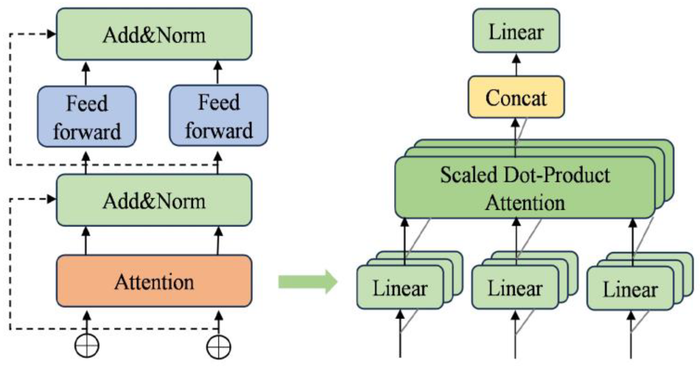
Figure 1. Transformer–multi-head attention.
Energies 17 03958 g001
Figure 2. GRU and BiGRU structure diagrams. (a) GRU structure diagram. (b) BiGRU structure diagram.
Energies 17 03958 g002
Figure 3. Global Attention structure.
Energies 17 03958 g003
Figure 4. Cross Attention structure.
Energies 17 03958 g004
Figure 5. Multi-level attention parallel architecture.
Energies 17 03958 g005
Figure 6. Clustering indicator.
Energies 17 03958 g006
Figure 7. Results of different weather model predictions. (a) Sunny day model prediction results. (b) Cloudy day model prediction results. (c) Rainy day model prediction results.
Energies 17 03958 g007
Table 1. Correlation coefficients between meteorological factors and output power.
Meteorological FactorsPearson Coefficient
Irradiance0.989
Temperature0.519
Humidity0.504
Wind speed0.346
Wind direction0.109
Air pressure0.058
Table 2. Clustering effect analysis.
AlgorithmDBIDITime
K-means0.1560.0200.670
ISODATA0.1230.0330.860
Improved ISODATA0.0570.0870.530
Table 3. Comparison of prediction results.
WeatherModelPavgRMSEMSEMAE R2IAEREScore
SunnyBiGRU46.6223.38811.4792.4290.995218.71740.9530.221
Transformer45.8673.51212.3352.9340.995265.23063.8270.193
BiGRU–Global Attention45.3933.18610.1532.6510.996199.10138.1900.268
CNN-LSTM46.1663.39311.5112.6820.995244.01646.1830.220
NARX46.3123.30710.9362.6390.995240.16253.9840.240
informer46.0783.32411.0462.8060.995255.29962.6390.236
Crossformer45.7923.17810.1012.4980.996227.35254.6730.270
Multi-level attention45.5653.1549.9452.0530.996184.91725.7300.275
CloudyBiGRU24.2974.22117.8213.1840.975283.40445.1910.037
Transformer25.3574.18917.5473.0920.975289.24553.7190.045
BiGRU–Global Attention23.6274.04916.3972.6910.977242.63231.8180.077
CNN-LSTM23.9954.09916.8002.9020.976264.09037.4200.065
NARX24.3514.44019.7133.0190.976293.89744.912−0.013
informer24.4923.95115.6142.8650.978260.73440.3930.099
Crossformer24.8123.75814.1242.6880.980244.63938.1990.143
Multi-level attention24.0823.72713.8892.1980.980196.01218.9790.150
RainyBiGRU13.9533.74614.0312.6440.959232.93441.5890.042
Transformer13.5363.70313.7092.6460.959231.80244.0030.053
BiGRU–Global Attention14.9232.8438.0822.0490.976185.54343.2760.273
CNN-LSTM14.4713.46912.0322.4610.965223.91347.3990.113
NARX14.0083.94115.5282.7080.954246.43039.696−0.008
informer14.2303.0759.4552.1400.972194.69238.0500.214
Crossformer14.4032.8227.9651.9740.977179.61635.3270.278
Multi-level attention13.9132.7887.7741.6920.977150.89124.9040.287
Disclaimer/Publisher’s Note: The statements, opinions and data contained in all publications are solely those of the individual author(s) and contributor(s) and not of MDPI and/or the editor(s). MDPI and/or the editor(s) disclaim responsibility for any injury to people or property resulting from any ideas, methods, instructions or products referred to in the content.