Article

Enhancing Lambda Measurement in Hydrogen-Fueled SI Engines through Virtual Sensor Implementation

Department of Engineering, University of Perugia, Via G. Duranti 93, 06125 Perugia, Italy
*
Author to whom correspondence should be addressed.
Energies 2024, 17(16), 3932; https://doi.org/10.3390/en17163932
Submission received: 2 July 2024 / Revised: 26 July 2024 / Accepted: 6 August 2024 / Published: 8 August 2024
(This article belongs to the Section I2: Energy and Combustion Science)

Abstract

:
The automotive industry is increasingly challenged to develop cleaner, more efficient solutions to comply with stringent emission standards. Hydrogen (H2)-powered internal combustion engines (ICEs) offer a promising alternative, with the potential to reduce carbon-based emissions and improve efficiency. However, hydrogen combustion presents two main challenges related to the calibration process: emissions control and measurement of the air excess coefficient (λ). Traditional lambda sensors struggle with hydrogen’s combustion dynamics, leading to potential inefficiencies and increased pollutant emissions. Consequently, the determination of engine performance could also be compromised. This study explores the feasibility of using machine learning (ML) to replace physical lambda sensors with virtual ones in hydrogen-fueled ICEs. The research was conducted on a single-cylinder spark-ignition (SI) engine, collecting data across a range of air excess coefficients from 1.6 to 3.0. An advanced hybrid model combining long short-term memory (LSTM) networks and convolutional neural networks (CNNs) was developed and fine-tuned to accurately predict the air–fuel ratio; its predictive performance was compared to that obtained with the backpropagation (BP) architecture. The optimal configuration was identified through iterative experimentation, focusing on the neuron count, number of hidden layers, and input variables. The results demonstrate that the LSTM + 1DCNN model successfully converged without overfitting; it also showed better prediction ability in terms of accuracy and robustness when compared with the backpropagation approach.

1. Introduction

The current regulations and guidelines on pollutant emissions are compelling the automotive industry to develop cleaner and more efficient solutions capable of reducing fuel consumption and emissions derived from internal combustion engines (ICEs) [1,2]. Among the options explored, hydrogen (H2)-powered alternative propulsion has emerged as promising candidate for the fossil-fuel-free future of mobility [3]. Hydrogen is a versatile, clean, and flexible energy source that can integrate renewables into the European grid by storing excess power, providing carbon-free fuel for transportation, replacing natural gas for heating, and supporting industrial feedstocks [4]. By 2050, hydrogen deployment could fill half the gap between current technology and the Paris Agreement goals, with Europe aiming for ambitious targets. Up to 2250 TWh of hydrogen could be generated by 2050, requiring 15–40 GW of water electrolysis capacity by 2030 to produce renewable hydrogen at less than EUR 3 per kg [5,6]. In a 2050 scenario, fuel cell electric vehicles (FCEVs) could dominate hydrogen demand, with over 4 million FCEVs on the road by 2030. The road transport sector, crucial for decarbonizing European economies, could see FCEVs reduce carbon emissions by over 40% in hydrogen applications by 2050 [6,7]. Unlike conventional fuels, H2 has the potential to eliminate carbon-based emissions while allowing for high efficiencies, also at challenging operating conditions like lean mixtures [8]. This is due to its high flame front propagation speed (with a laminar burning velocity approximately six times greater than that of gasoline E5) and broad flammability limits [9]. Hydrogen offers also multiple application modes within internal combustion engines [10], as explored in various studies focusing on its use either as a primary fuel or in combination with fossil fuels to boost efficiency and reduce emissions [11]. The ability of hydrogen engines to sustain higher compression ratios, up to 14.5:1, due to highly diluted mixtures and a high autoignition temperature results in superior thermodynamic efficiency, potentially reaching 52% [12]. For instance, Shi et al. [13] reported an increase in brake thermal efficiency from approximately 10.0% to 16.7% with a 6% hydrogen addition to gasoline under an excess air ratio of 1.3 in a modified Wankel engine. Dimitriou et al. [14] also observed a peak brake thermal efficiency improvement of approximately 3% with an 80% hydrogen energy addition. When pure hydrogen is used, emissions of hydrocarbons (HCs) and carbon monoxide (CO) are nearly eliminated, with only minor contributions from the combustion of lubricating oil [15,16]. However, the intrinsic characteristics of hydrogen combustion makes the calibration of hydrogen-fueled engines difficult due to their combustion dynamics and emission control mechanisms [17]. Ones of the challenges in hydrogen combustion regards the propensity for misfires and delayed combustion at the exhaust port, which leads to inefficiencies in engine operation as well as increased pollutant emissions [18,19]. Verhelst et al. [20] reported that an unoptimized spark plug in a hydrogen engine caused misfires, leaving unburned hydrogen in the cylinder, which led to backfire in the next cycle. Gao et al. [21] discovered that a misfire in one cylinder could result in severe knocking in the same and other cylinders. The unburned mixture from the misfire cycle burns in the exhaust system, producing oscillating waves that cause knocking in the cylinders. These anomalies make the traditional lambda sensors unable to accurately identify the oxygen concentration in the exhaust gases to determine the air excess coefficient (λ) [22,23].
Within this context, machine learning (ML) solutions can be exploited to address such an issue. The capability of ML algorithms to analyze complex data patterns starting from input variables makes them well-suited for tasks such as λ prediction in H2-ICE. In such a way, the exploitation of virtual sensors [24,25,26] can mitigate the impact of lambda sensors malfunctioning and response delays [27,28]. Wong et al. [29] proposed an adaptive air–fuel ratio control method employing extreme machine learning (EML), which was fine-tuned through simulations and experiments on a retrofitted spark-ignition (SI) dual-injection engine. The ELM-based controller outperforms traditional PID controllers, offering significant advancements in engine control technology. McGann et al. [30] developed a predictive model using an ML approach to detect the fuel–air equivalence ratio (ϕ) and pressure derived from the laser-induced plasma spectra. Quantitative outcomes showed R2 values of up to 0.99996 for ϕ and 0.99975 for pressure, demonstrating high predictive performance and the efficacy of the presented model. Wong et al. [31] demonstrated, through simulations and experimental activities, the effectiveness of an initial-training-free online sequential extreme learning machine (ITF-OSELM) in identifying air–fuel ratio dynamics in real-time engine data and in calculating control signals for air–fuel regulation.

Present Contribution

This study examines the feasibility of replacing the physical lambda sensor with a virtual one to avoid problems due to sensor malfunctions, enhance the reliability of estimating the air excess coefficient, and compensate for any delays due to the probe time response. Tests were conducted on a SI single-cylinder research engine fueled with H2, spanning a wide range of relative λ from 1.6 to 3.0. The experimental setup involves collecting data coming from an indicated analysis system. These data are used as the input for the machine learning algorithms, which are trained to predict the air excess index based on the observed engine behavior. To perform this task, a long short-term memory (LSTM) [32,33] approach combined with a convolutional neural network (CNN) [34,35] has been used. Fukuoka et al. [36] utilized a combination of 1D-CNN and LSTM to forecast wind speed in Tokushima city. Typically, wind speed is monitored over a specific timeframe, and their method leverages historical data to predict current conditions. In a separate study, Rosato et al. [37] introduced a pioneering deep learning method combining long short-term memory networks and convolutional neural networks, which was developed to forecast energy patterns in a practical solar power plant. Following a thorough assessment, their framework emerged as a reliable and efficient solution for predictive applications. Its notable advantage lies in its utilization of effective and intelligent strategies to leverage various physical data sources. In our investigation, documented as [38], we devised a hybrid model employing LSTM and 1DCNN to explore the viability of replacing a physical sensor such as a torque meter with a virtual alternative. Successfully achieving this goal could result in substantial cost reductions and protect test bench components from damage caused by resonance phenomena, as noted in the references [39,40]. This model accurately reproduces the natural frequency of recorded signals, assuring that the predicted values consistently deviate within the acceptable threshold of 10% from actual values. Furthermore, our research group evaluated the predictive performance of LSTM + 1DCNN in forecasting in-cylinder pressure traces of a three-cylinder spark-ignition engine across various operational conditions. The results underscore the superior capability of LSTM + 1DCNN in capturing the trends in target signals. When compared to alternative benchmark architectures, our model consistently demonstrates superior performance, achieving average error rates below 2%. Notably, even as engine variability increases from cycle to cycle, LSTM + 1DCNN maintains average error rates below 1.5%, highlighting its robustness and reliability in predictive accuracy [41].
In the present work, research on fine-tuning parameters such as the number of neurons, hidden layers, and input variables in neural network models has been performed to maximize prediction accuracy. Through iterative experimentation and validation, the optimal configuration of the machine learning algorithms has been identified, as has its respective performance compared to those from other optimized machine learning architectures.
The results show that the LSTM + 1DCNN model successfully reaches convergence during training without experiencing overfitting, showcasing its ability to learn effectively from the data and produce precise predictions. Moreover, it exhibits superior accuracy, robustness, and prediction performance compared to the backpropagation structure. These findings indicate that LSTM + 1DCNN holds considerable promise for predicting exhaust oxygen concentrations in spark-ignition engines.

2. Materials and Methods

2.1. Experimental Setup

The experimental campaign was performed on a 500 cc single-cylinder engine, depicted in Figure 1, equipped with four valves and featuring a pent-roof combustion chamber and a reverse tumble intake port system. The latter is specifically designed for operation in both direct injection (DI) [38] and port fuel injection (PFI) [42] modes. Additional specifications regarding the test engine are available in Table 1 [43]. The tests were carried out at 1000 rpm in PFI mode with centrally positioned igniters.
A throttle valve positioned upstream of the intake manifold regulated the airflow rate, with its configuration remaining constant for all the test points, specifically taking into account a throttle valve opening (TVO) of 10%. This ensured consistent airflow towards the combustion chamber and unchanged in-cylinder charge motion [42]. The air excess coefficient was adjusted exclusively by modifying the quantity of hydrogen fuel injected, maintained at a fixed injection pressure of 4 bar absolute. Below, the remaining components of the experimental apparatus are listed and outlined, with their schematic arrangement and associated connections depicted in Figure 2. An Athena GET HPUH4 engine control unit (ECU) has been used to regulate the timing of injector activation and ignition timing. This ECU achieved control by sending a trigger signal to the ignition control unit. For combustion analysis, the Kistler KiBox system was employed, featuring an angular resolution of 0.1 CAD. This system gathered several critical data types: intake port pressure was measured using a Kistler 4075A5 (Kistler Group: Winterthur, Switzerland) piezoresistive transducer; in-cylinder pressure was recorded with a Kistler 6061B (Kistler Group: Winterthur, Switzerland) piezoelectric transducer; and the absolute crank angle position was determined using an AVL 365C optical encoder (IndiaMART: Noida, India). Additionally, the oxygen percentage was measured with a Horiba Mexa 720 fast probe (HORIBA, Ltd.: Kyoto, Japan), with an accuracy of ±0.5%, while the ignition signal was provided by the ECU.
For the study, a conventional spark plug prototype was chosen as the igniter.

2.2. Estimation of the Relative Air Excess Coefficient

Throughout the course of the engine’s operations, the activation time value of the injector (ton) was finetuned to attain the desired target of λ, guided by the concentration of O2% in the combustion process furnished by the Horiba MEXA-720, as specified in the previous paragraph, using the equation derived from the complete combustion of hydrogen and oxygen and rearranged by Azeem et al. [22] as reported in Equation (1):
λ = 1 + X O 2 1 X O 2 Y O 2
where X O 2 represents the oxygen wet concentration in the exhaust gas and Y O 2 indicates the corresponding concentration in the intake air, which stands at around 21%. Such a type of regulation is deemed necessary owing to the impossibility of flushing the injector and the absence of a “fuel meter”, which allows the quantification of the injected fuel mass flow rate ( m c ˙ ) and therefore direct adjustment of the λ value.

2.3. Definition of the Case Study for the Output Prediction

2.3.1. Definition of the Involved Parameters

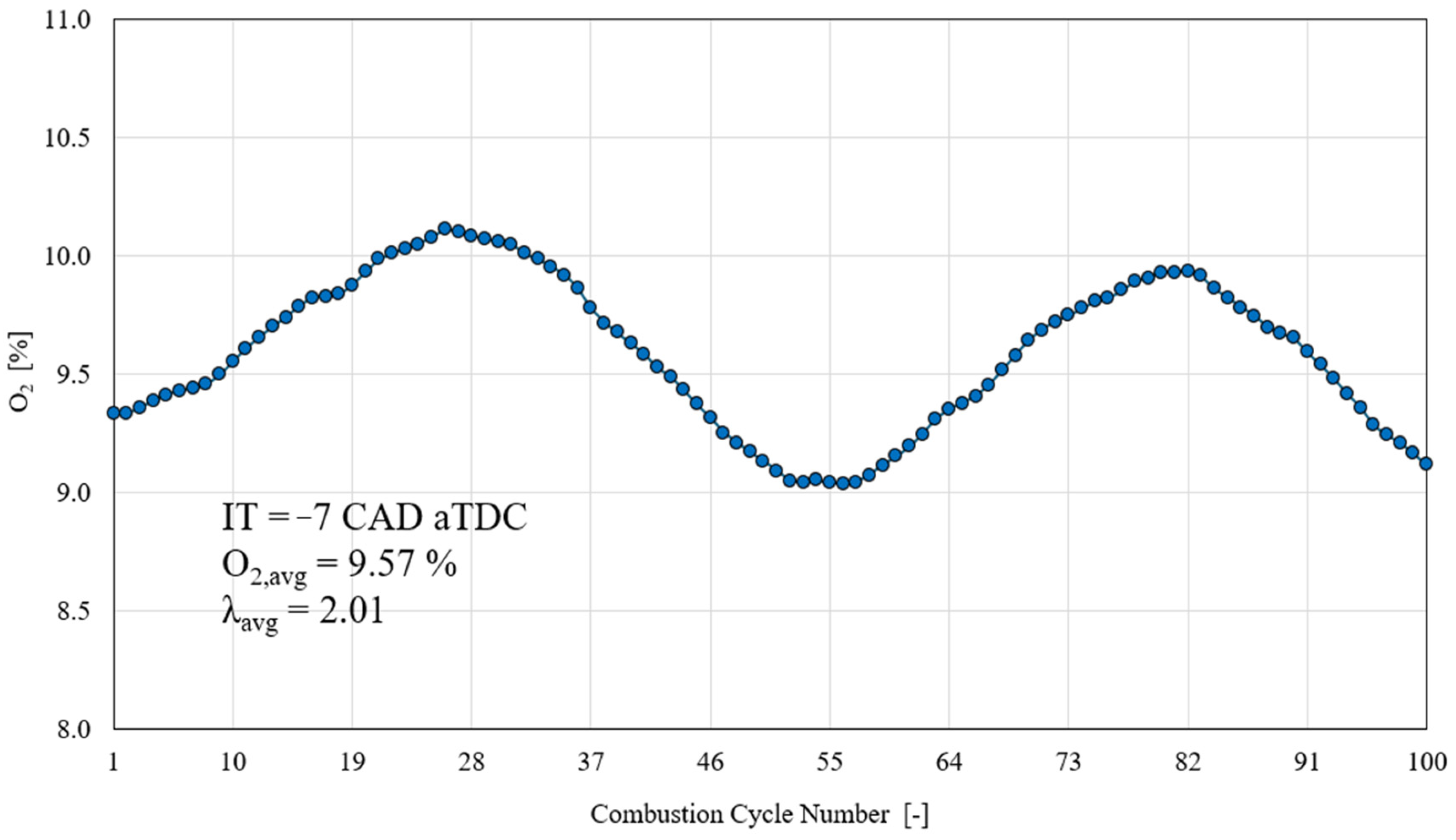
In this work, the performance of an LSTM-CNN structure in predicting the λ at the exhaust pipe of a spark-ignition engine (Figure 3) has been evaluated and compared with the ones coming from other ML architectures.
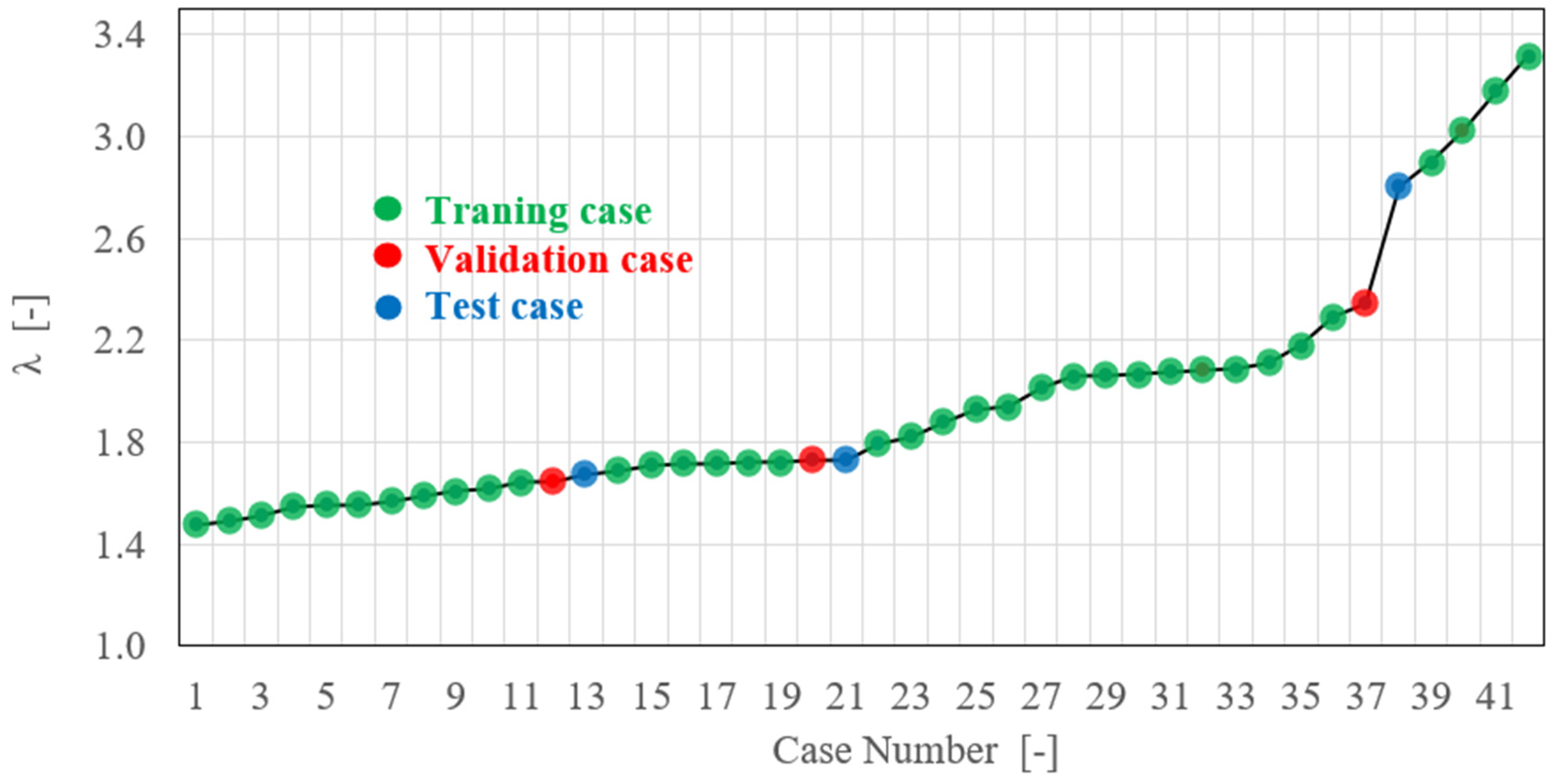
The initial dataset is composed by data coming from experiments conducted at different λ values, from 1.5 to 3.5 (Figure 4). Each tested operating point is characterized by the coefficient of variance (CoV) of the indicated mean effective pressure (IMEP) being lower than 3% [44]. The threshold enables the operating point to be considered as fully stable.
The initial dataset, described in Table 2, is composed of 42 operating cases. For each operating case, a total of 100 consecutive combustions were recorded by the Kibox analysis system. For each combustion event, the following 8 parameters served as an input for the ML structure:
  • Ignition timing, IT (CAD aTDC).
  • Crank angle degree (CAD) after top dead center (aTDC), for which 5% of the mass fraction (MF) is burned, AI05 (CAD aTDC).
  • CAD aTDC, for which 50% of MF is burned, AI50 (CAD aTDC).
  • CAD aTDC, for which 90% of MF is burned, AI90 (CAD aTDC).
  • CAD aTDC in correspondence of the maximum in-cylinder pressure, APmax (CAD aTDC).
  • Maximum in-cylinder pressure, Pmax (bar).
  • Indicated mean effective pressure, IMEP (bar).
  • Injector activation time, ton (μs).
Due to the inability to retroactively control the injector activation time, it has been fixed based on the target lambda value. Therefore, it is essential to predict the exhaust oxygen concentration accurately with an ML approach to enable the control of the injector timing.
Considering the observations reported in Figure 4 and Figure 5 and the subdivision of the initial dataset shown in Table 2, which consists of 42 × [100 × 8] input variables and 42 × [100 × 1] output variables, the dataset was divided into test, validation, and training sets.

2.3.2. Evaluating the Influence of the Input Parameters on the Output Prediction

By removing variables with minimal correlation, the model’s dimensions can be effectively reduced, thereby improving its accuracy. To accomplish this goal, an initial analysis utilizing the Shapley value was performed on the entire dataset. SHAP is used to clarify the prediction of an instance by assessing the contribution of each feature. By excluding variables with weak correlation, the model’s dimensions can be effectively reduced, thereby improving its accuracy. The researchers also evaluated the average absolute Shapley values (ABSVs) to determine the influence of individual measured quantities on the objective function [45,46]. The results shown in Figure 6 indicate that ton is the most influential parameter for predicting λ, followed by the maximum in-cylinder pressure (percentage of impact: 47%), APmax, AI50, and IMEP. On the other hand, AI05, AI90, and IT, highlighted in red in Figure 6, are the least influential parameters, with impact percentages below 5%.
Consequently, these three parameters were excluded from the final dataset, reducing the count of inputs from 8 to 5. Earlier studies conducted by the same team of research [38,41] revealed improvements in predictive capabilities when parameters with marginal influence were excluded. Accordingly, this study centers on evaluating the predictive accuracy of the architecture using the five previously identified input parameters: AI50, APmax, IMEP, Pmax, and ton. After analyzing the input parameters, a normalization procedure is implemented to mitigate prediction errors and expedite the architecture’s convergence. This method mitigates discrepancies between input and output parameters by scaling values to the range [0, 1]. Following the prediction procedure, a data de-normalization process must be undertaken to enable direct comparison between the predicted values and the original target values.

2.3.3. Definition of the Final Dataset for the Output Prediction

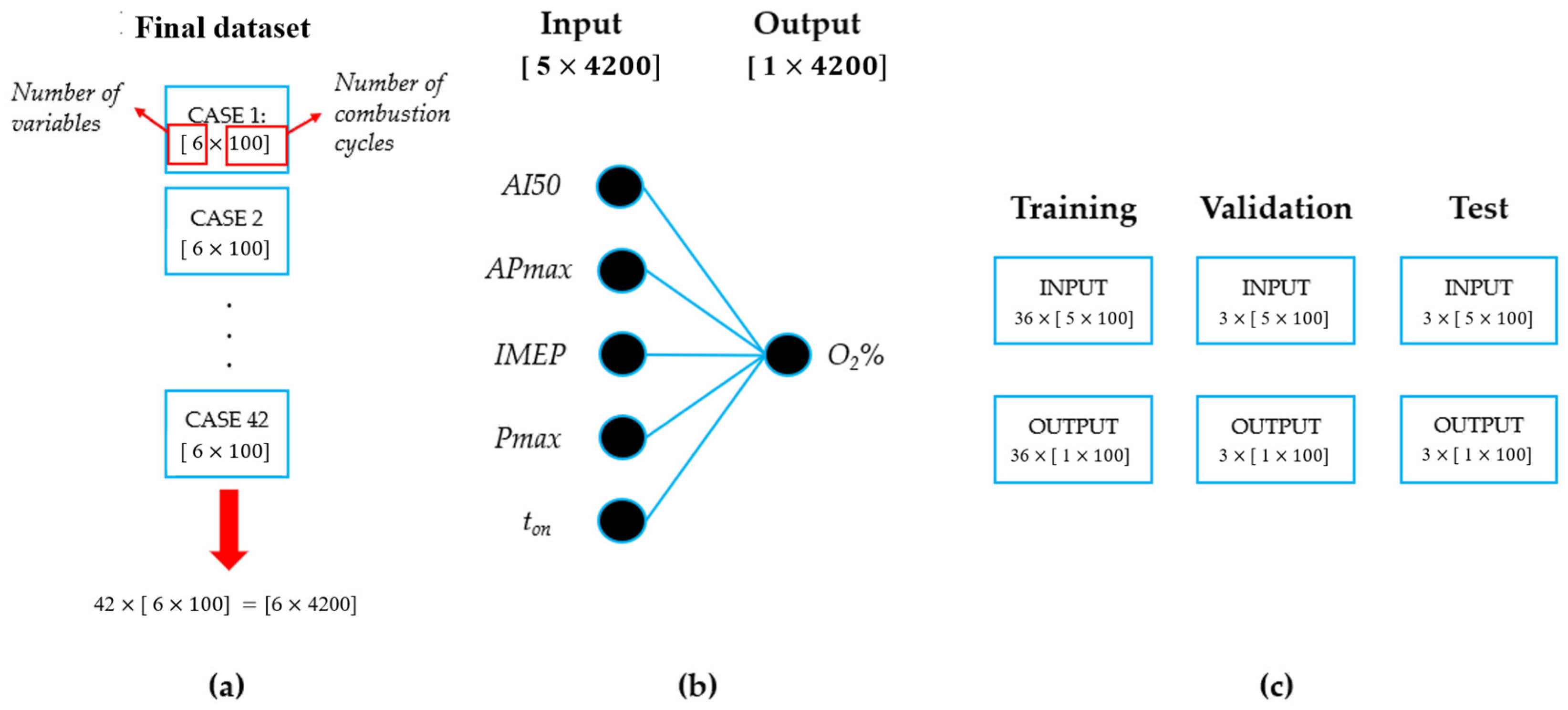
On the basis of the sensitivity analysis results outlined in the preceding paragraph and summarized in Figure 5, Figure 7 offers a detailed summary of the final dataset and, additionally, for each case examined, the arrangement of input and output parameters. As shown in Figure 7a, the dataset consists of 42 experimental cases specified in Table 2, with every single case characterized by 6 variables. Each variable includes 100 samples, corresponding to the number of combustion cycles. The input parameters, AI50, APmax, IMEP, Pmax, and ton, form a 42 × [5 × 100] matrix, while the output parameter forms a 42 × [1 × 100] matrix (Figure 7b). The dataset was divided such that 80% of the data was utilizing for training, 10% for validation, and the remaining 10%, 3 × [5 × 100], was used for testing to predict the output, 3 × [1 × 100] (Figure 7c).

3. Creating the Artificial Architecture to Perform Output Prediction

3.1. LSTM + 1DCNN Structure

Figure 8a illustrates the forecasting model of LSTM + 1DCNN utilized for predicting the output and subsequently determining the operative λ value. The process begins with a sequence input layer that feeds the dataset inside the neural network, defining its dimensions and creating the required structures. Following this, a one-dimensional CNN layer employs a “1D convolutional filter” on each frame of input, which is composed of neurons and uses a “ReLu activation function” [47,48]. The procedure then involves an “average pooling layer” that computes the mean values of patches in a feature map, reducing the maps size (i.e., “down-sampling”), utilizing the mean value in 2 × 2 cell squares. This is followed by another 1D convolutional layer, similar to the earlier one. An LSTM layer with hidden units then handles the feature maps. Gates play a vital role in the inner structure of the LSTM network, as depicted in Figure 8b. Using data from the prior layer (ht−1) and the current input (xt), the “forget gate” determines which information should be kept or removed. A sigmoid function processes this data, yielding an output between 0 and 1 to determine if the information should be retained. This gate modifies the prior cell state value (Ct−1). The “input gate” then identifies which information to save in the “cell state” through several steps. Initially, the “input port layer” employs a Sigmoid function (σ) to decide which values to update. Subsequently, a new set of candidate values (Ct) is created using a Hyperbolic Tangent function (tanh). These two sets of values are combined and updated using the Forget function (ft), replacing the old cell state (Ct−1) with the new one (Ct). The updated cell state is then multiplied by the Forget function (ft). The output gate retains a filtered version of the processed data, with the Sigmoid function determining which parts of the cell state to output. The cell state undergoes a tanh operation to limit values between −1 and 1, which are subsequently multiplied by the “Sigmoid gate output”, resulting in the final output (yt) of only the selected parts. LSTMs feature a unique structure with a “Forget gate activation”, allowing the network to encourage desired behavior through frequent updates at each learning stage. After the LSTM layer completes its process, the “time-distributed layer” segments the feature map into a sequence of temporal vectors. Finally, the “regression output layer” calculates the “mean square error loss” to solve the regression problem, with ht representing the new layer and yt the current output, i.e., the predicted value.

3.2. Definition of the Procedures to Determine the Structural Parameters of the Proposed Models

The optimized neural architectures are defined based on preliminary analysis of training session performance. The effectiveness of the model’s parameters is measured using the mean square error (MSE) as the loss metric (Equation (2)):
M S E = 1 N i = 1 N ( Y p r e d i c t e d i Y t a r g e t i ) 2
where:
  • N = number of combustion cycles;
  • i = ith combustion cycle;
  • Y p r e d i c t e d i = predicted value;
  • Y t a r g e t i = target value (gleaned from experiments).
The network is trained for 10,000 epochs, allowing the final loss function value, for each prediction model, to be computed upon reaching the maximum learning iteration.
For the LSTM + 1DCNN architecture, various structural parameters are investigated: the number of neurons in the 1DCNN layers (Nc) ranges from 50 to 200, the neurons in the LSTM hidden layers (Nh) also span from 50 to 200, the batch size (Bs) varies between 8 and 64, and the model depth (Md) extends from 1 to 5 layers.
The “Adam optimizer”, which includes adaptive learning rate adjustments during training, is utilized to refine the weight matrix and biases in the LSTM model.
A “MaxPooling1D layer” composed of pool_size = 2 and strides = 2 has been located between the CNN and LSTM layers.
A “time-distributed layer” has been used after the LSTM layer. It applies a “fully connected (dense) layer” with one unit to each time step of the input sequence independently. This is useful for sequence data where each time step needs to be processed separately, such as in sequence prediction tasks where each time step has its own prediction.
A “dense (units = 1) layer”, a standard fully connected layer with one unit, has ultimately been used as the output layer since a single scalar output is required.
The most effective configurations, identified by the lowest mean square error (MSE) values, were selected for predicting λ, resulting in Nc = 134, Nh = 38, Bs = 1, and Md = 2.
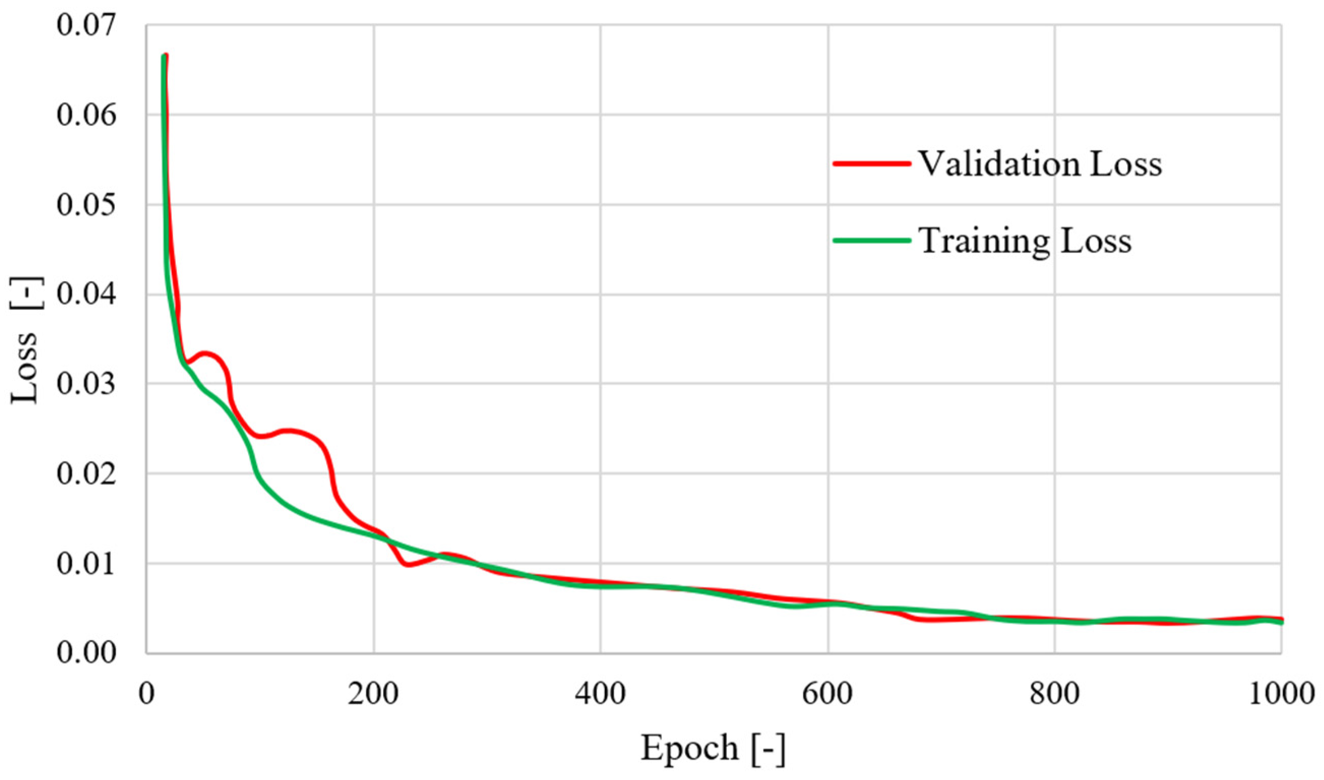
For the sake of completeness, Figure 9 displays the validation loss and training loss for the best-performing LSTM + 1DCNN structure.
The performance of this proposed architecture is evaluated against an alternative approach, specifically the backpropagation model. The BP algorithm [49,50,51] features an architecture with one input layer; three hidden layers containing 50, 87, and 11 neurons, respectively; and a single output layer. Similar to the LSTM + 1DCNN architecture, this configuration was fine-tuned through a thorough preliminary analysis.

4. Results and Discussion

Figure 10 depicts the predictions of λ, starting from the prediction of oxygen concentration according to Equation (1), for the three testing cases performed by the two neural structures analyzed.
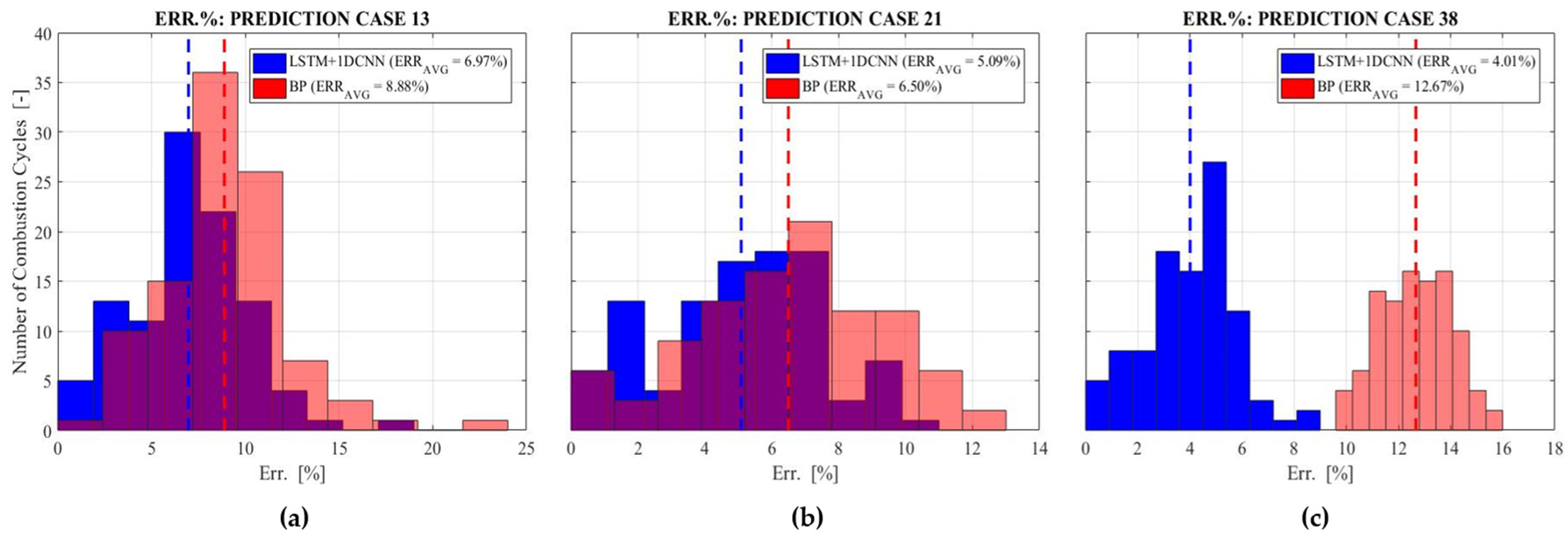
To ensure clarity, prediction, concerning the entirety of events, was carried out for operational cases 13, 21, and 38, each characterized by 100 combustion cycles. For all of the aforementioned cases, both test structures are capable of reproducing the trend in the oxygen concentration over the considered combustion cycles. Examining the details more closely, it is evident that the LSTM + 1DCNN architecture achieves predictions that are closer to the target across all three analyzed cases compared to the BP structure. Furthermore, as corroborated by the error graphs in Figure 11, the LSTM + 1DCNN architecture progressively improves the prediction performance as the mixture becomes leaner, with the RMSE (Root Mean Square Error) [41] decreasing from 3.16% (case 13, Figure 10a) to 2.72% (both cases 21 and 38, Figure 10b and Figure 10c, respectively). Conversely, while the BP model shows slightly different trends from LSTM + 1DCNN for cases 13 and 21, it performs significantly worse for case 38, with an RMSE of 8.27%, greatly underestimating the target value.
The percentage error of the ith operating case, indicated as Err, defined as the distance between the approximate value and the exact value as a percentage of the actual value, has been determined using Equation (3):
E r r ( i ) = | Y p r e d i c t e d i Y t a r g e t i | Y t a r g e t i × 100
The average percentage error, referred to as Erravg and evaluated utilizing Equation (4), is computed to evaluate the overall accuracy of predictions:
E r r a v g = 1 N i = 1 N | Y p r e d i c t e d i Y t a r g e t i | Y t a r g e t i × 100
To ensure accurate predictions, a strict upper limit of 10% is set for these calculated errors to maintain high-quality standards.
As illustrated in Figure 11a,b, BP demonstrates an Erravg of 8.88% for case 13 and 6.50% for case 21, both of which are below the critical threshold of 10%. Specifically, 33 cycles and 11 cycles, respectively, or approximately 33% and 11% of the predicted combustion cycles, exhibit an Err(i) exceeding 10%. However, in case 38 (Figure 11c), BP exhibits an Erravg of 12.67%, significantly exceeding the critical threshold of acceptability. The LSTM + 1DCNN model enhances BP performance, consistently demonstrating an Erravg below that of the BP architecture and the critical threshold. Specifically, the Erravg is 6.97% for case 13, 5.09% for case 21, and 4.01% for case 38. Furthermore, it is important to emphasize that as the mixture is leaner, the LSTM + 1DCNN structure progressively improves the prediction performance, achieving zero cycles beyond the critical threshold of 10% for case 38.
The regression accuracy (R2) pertaining to the predictions generated by the two architectures tested, illustrated in Figure 12, has been calculated using Equation (5).
R 2 = 1 i = 1 N ( Y p r e d i c t e d i Y t a r g e t i ) 2 i = 1 N ( Y t a r g e t i Y ¯ t a r g e t ) 2
where Y ¯ t a r g e t = mean of the target values.
As can be observed, the data points in all charts are plotted with the predicted values on the y-axis and the target values on the x-axis. The closer the points are to the diagonal dashed line, the more accurate the predictions are. Each plot uses a scale appropriate to the data range of the respective case. Both models demonstrate high accuracy in the lower-to-medium range of analysis, specifically at low λ levels. As the oxygen concentration increases, BP shows greater dispersion (R2 = 0.9802, case 38), whereas LSTM + 1DCNN exhibits a consistent distribution along the interpolation line without significant deviations (R2 = 0.9974, case 38). Notably, this architecture exhibits minimal dispersion, with an R2 value approaching unity, specifically R2 = 0.9996 for case 21, which is higher than the value achieved for the same case using BP (R2 = 0.9992). These findings underscore the superior linear fitting and predictive accuracy of the LSTM + 1DCNN architecture compared to the BP architecture across all three cases examined. The findings underscore the strong learning capabilities of the LSTM + 1DCNN architecture, demonstrating its proficiency in faithfully reproducing the target trend throughout the learning process.

Challenges and Opportunities

While machine learning shows promise for enhancing emission control in hydrogen combustion engines, several challenges remain. One key challenge is the need for large amounts of high-quality data for training and validating machine learning models. Collecting representative data from diverse operating conditions and engine configurations is essential to ensure the robustness and generalization of the models.
Additionally, the integration of machine learning algorithms into real-time engine control systems presents technical and logistical challenges. Ensuring the reliability, safety, and compatibility of machine-learning-based systems with existing engine architectures requires careful consideration and validation.
Despite these challenges, the potential benefits of machine learning for emission control in hydrogen combustion engines are substantial. By providing accurate and reliable λ predictions, virtual lambda sensors can enable more precise control of combustion processes, leading to improved engine performance and reduced emissions. Furthermore, machine-learning-based approaches have the flexibility to adapt to changing operating conditions and optimize engine performance in real time, offering opportunities for continuous improvement and innovation in emission control strategies.

5. Conclusions

The current study assessed the LSTM + 1DCNN model’s efficacy for the λ prediction at the exhaust pipe of a single-cylinder spark-ignition engine across different operational scenarios. The aim was to explore the potential of advanced machine learning techniques as substitutes for physical sensors and to assess the feasibility of integrating virtual lambda sensors into onboard control systems. This approach may reduce the need for costly and time-intensive structural alterations.

Main Findings

The findings gleaned from the present comparative analysis demonstrate the superior performance of the LSTM + 1DCNN model in replicating target signal trends. In particular, compared to the backpropagation approach, this model consistently exhibits the highest accuracy, with average error percentages below 10%. As the air–fuel mixture is progressively leaned, the LSTM + 1DCNN model achieves average error percentages equal to approximately 4%, while that of the BP structure increases by up to roughly 13%. This research found that the LSTM + 1DCNN architecture can achieve convergence during training without experiencing overfitting, showcasing its ability to learn efficiently from input data and predict with high precision. Additionally, it demonstrates superior accuracy and robustness compared to the backpropagation structure. These findings suggest that LSTM + 1DCNN holds great potential for accurately forecasting the air excess coefficient (λ) in SI engines.
In conclusion, integrating machine learning in hydrogen combustion engines shows great promise for advancing emission control. Virtual lambda sensors can address sensor malfunctions and response delays. Experimental validation on single-cylinder engines demonstrates the potential of these techniques for improving performance and reducing emissions, paving the way for a cleaner, more sustainable automotive future.

Author Contributions

Conceptualization, F.R. and F.M.; methodology, F.R. and M.A.; software, F.R. and M.A.; validation, F.M.; formal analysis F.R.; investigation, F.R. and M.A.; resources, F.M.; data curation, F.R. and M.A.; writing—original draft preparation, F.R. and M.A.; writing—review and editing, F.R., M.A. and F.M.; visualization, F.R. and M.A.; supervision, F.M.; project administration, F.M. All authors have read and agreed to the published version of the manuscript.

Funding

This research received no external funding.

Data Availability Statement

Dataset available on request from the authors.

Conflicts of Interest

The authors declare no conflicts of interest.

Nomenclature

1D-CNNOne-dimensional CNN
ABSVAverage absolute Shapley value
aBDCafter bottom dead center
AI05Crank angle degree after the top dead center (TDC), for which 5% of the mass is burned
AI50Crank angle degree after the top dead center (TDC), for which 50% of the mass is burned
AI90Crank angle degree after the top dead center (TDC), for which 90% of the mass is burned
APmaxCrank angle degree after the top dead center (TDC), where the maximum in-cylinder pressure is recorded
aTDCafter top dead center
BsBatch size
CADCrank angle degree
CNNConvolutional neural network
CoVIMEPCoefficient of variance of IMEP
DIDirect injection
EMLExtreme machine learning
ECUEngine control unit
ErrPercentage error
ErravgAverage percentage error
ϕFuel–air equivalence ratio
H2Hydrogen
ICEInternal combustion engine
IMEPIndicated mean effective pressure
ITIgnition timing
ITF-OSELMInitial-training-free online sequential extreme learning machine
λ (1/φ)Air excess coefficient
LSTMLong short-term memory
LSTM + 1DCNN1D-CNN and LSTM model combination
mcInjected fuel mass flow rate
MdModel depth
MLMachine learning
NcNumber of neurons in the 1DCNN layers
NhNumber of neurons in the LSTM hidden layers
MSEMean square error
O2Oxygen
PFIPort fuel injection
PmaxMaximum in-cylinder pressure
R2Coefficient of determination
RMSERoot mean square error
SHAPShapley analysis
SISpark ignition
tonActivation time

References

  1. Suresh, D.; Porpatham, E. Influence of high compression ratio and hydrogen addition on the performance and emissions of a lean burn spark ignition engine fueled by ethanol-gasoline. Int. J. Hydrogen Energy 2023, 48, 14433–14448. [Google Scholar] [CrossRef]
  2. Reitz, R.D.; Ogawa, H.; Payri, R.; Fansler, T.; Kokjohn, S.; Moriyoshi, Y.; Agarwal, A.; Arcoumanis, D.; Assanis, D.; Bae, C.; et al. IJER editorial: The future of the internal combustion engine. Int. J. Engine Res. 2020, 21, 3–10. [Google Scholar] [CrossRef]
  3. Duan, X.; Xu, L.; Xu, L.; Jiang, P.; Gan, T.; Liu, H.; Ye, S.; Sun, Z. Performance analysis and comparison of the spark ignition engine fueled with industrial by-product hydrogen and gasoline. J. Clean. Prod. 2023, 424, 138899. [Google Scholar] [CrossRef]
  4. Joshi, A. Review of vehicle engine efficiency and emissions. SAE Int. J. Adv. Curr. Pract. Mobil. 2020, 2, 2479–2507. [Google Scholar] [CrossRef]
  5. Campos-Carriedo, F.; Bargiacchi, E.; Dufour, J.; Iribarren, D. How can the European Ecodesign Directive guide the deployment of hydrogen-related products for mobility? Sustain. Energy Fuels 2023, 7, 1382–1394. [Google Scholar] [CrossRef]
  6. Anika, O.; Nnabuife, S.; Bello, A.; Okoroafor, E.; Kuang, B.; Villa, R. Prospects of low and zero-carbon renewable fuels in 1.5-degree net zero emission actualization by 2050: A critical review. Carbon Capture Sci. Technol. 2022, 5, 100072. [Google Scholar] [CrossRef]
  7. Statistical Office of the European Union. Energy, Transport and Environment Statistics: 2020 Edition. 2020. Available online: https://ec.europa.eu/eurostat/web/products-statistical-books/-/KS-DK-20-001 (accessed on 1 July 2024).
  8. Ceviz, M.A.; Kaymaz, I. Temperature and air-fuel ratio dependent specific heat ratio functions for lean burned and unburned mixture. Energy Convers. Manag. 2005, 46, 2387–2404. [Google Scholar] [CrossRef]
  9. Sementa, P.; Antolini, J.B.d.V.; Tornatore, C.; Catapano, F.; Vaglieco, B.M.; Sánchez, J.J.L. Exploring the potentials of lean-burn hydrogen SI engine compared to methane operation. Int. J. Hydrogen Energy 2022, 47, 25044–25056. [Google Scholar] [CrossRef]
  10. Srinivasan, C.B.; Subramanian, R. Hydrogen as a Spark Ignition Engine Fuel Technical Review. Int. J. Mech. Mechatron. Eng. IJMME-IJENS 2014, 14, 111–117. [Google Scholar]
  11. Aydin, K.; Kutanoglu, R. Effects of hydrogenation of fossil fuels with hydrogen and hydroxy gas on performance and emissions of internal combustion engines. Int. J. Hydrogen Energy 2018, 43, 14047–14058. [Google Scholar] [CrossRef]
  12. Verhelst, S.; Sierens, R.; Verstraeten, S. A Critical Review of Experimental Research on Hydrogen Fueled SI Engines. SAE Trans. 2006, 115, 264–274. [Google Scholar]
  13. Shi, C.; Ji, C.; Wang, S.; Yang, J.; Wang, H. Experimental and numerical study of combustion and emissions performance in a hydrogen-enriched Wankel engine at stoichiometric and lean operations. Fuel 2021, 291, 120181. [Google Scholar] [CrossRef]
  14. Dimitriou, P.; Kumar, M.; Tsujimura, T.; Suzuki, Y. Combustion and emission characteristics of a hydrogen-diesel dual-fuel engine. Int. J. Hydrogen Energy 2018, 43, 13605–13617. [Google Scholar] [CrossRef]
  15. Wu, H.; Yu, X.; Du, Y.; Ji, X.; Niu, R.; Sun, Y.; Gu, J. Study on cold start characteristics of dual fuel SI engine with hydrogen direct-injection. Appl. Therm. Eng. 2016, 100, 829–839. [Google Scholar] [CrossRef]
  16. Serin, H.; Yıldızhan, Ş. Hydrogen addition to tea seed oil biodiesel: Performance and emission characteristics. Int. J. Hydrogen Energy 2018, 43, 18020–18027. [Google Scholar] [CrossRef]
  17. Gao, J.; Wang, X.; Song, P.; Tian, G.; Ma, C. Review of the backfire occurrences and control strategies for port hydrogen injection internal combustion engines. Fuel 2022, 307, 121553. [Google Scholar] [CrossRef]
  18. Diéguez, P.M.; Urroz, J.; Sáinz, D.; Machin, J.; Arana, M.; Gandía, L. Characterization of combustion anomalies in a hydrogen fueled 1.4 L commercial spark-ignition engine by means of in-cylinder pressure, block-engine vibration, and acoustic measurements. Energy Convers. Manag. 2018, 172, 67–80. [Google Scholar] [CrossRef]
  19. Ye, Y.; Gao, W.; Li, Y.; Zhang, P.; Cao, X. Numerical study of the effect of injection timing on the knock combustion in a direct-injection hydrogen engine. Int. J. Hydrogen Energy 2020, 45, 27904–27919. [Google Scholar] [CrossRef]
  20. Verhelst, S.; Demuynck, J.; Sierens, E.; Huyskens, P. Impact of variable valve timing on power, emissions and backfire of a bi-fuel hydrogen/gasoline engine. Int. J. Hydrogen Energy 2010, 35, 4399–4408. [Google Scholar] [CrossRef]
  21. Gao, J.; Yao, A.; Zhang, Y.; Qu, G.; Yao, C.; Zhang, S.; Li, D. Investigation into the relationship between super-knock and misfires in an SI GDI engine. Energies 2021, 14, 2099. [Google Scholar] [CrossRef]
  22. Azeem, N.; Beatrice, C.; Vassallo, A.; Pesce, F.; Davide, G.; Guido, C. Comparative Analysis of Different Methodologies to Calculate Lambda (λ) Based on Extensive And systemic Experimentation on a Hydrogen Internal Combustion Engine. In SAE Technical Paper; 2023-01-0340; SAE: Pittsburgh, PA, USA, 2023. [Google Scholar] [CrossRef]
  23. Peters, N.; Bunce, M. Lambda Determination Challenges for Ultra-Lean Hydrogen-Fueled Engines and the Impact on Engine Calibration (No. 2023-01-0286). In SAE Technical Paper; SAE: Pittsburgh, PA, USA, 2023. [Google Scholar]
  24. Abu-Nabah, B.A.; ElSoussi, A.O.; Abed, E.K.; Alami, A.l. Virtual laser vision sensor environment assessment for surface profiling applications. Measurement 2018, 113, 148–160. [Google Scholar] [CrossRef]
  25. Huang, G.; Fukushima, E.F.; She, J.; Zhang, C.; He, J. Estimation of sensor faults and unknown disturbance in current measurement circuits for PMSM drive system. Measurement 2019, 137, 580–587. [Google Scholar] [CrossRef]
  26. Bai, S.; Li, M.; Lu, Q.; Fu, J.; Li, J.; Qin, L. A new measuring method of dredging concentration based on hybrid ensemble deep learning technique. Measurement 2022, 188, 110423. [Google Scholar] [CrossRef]
  27. Pan, H.; Xu, H.; Liu, Q.; Zheng, J.; Tong, J. An intelligent fault diagnosis method based on adaptive maximal margin tensor machine. Measurement 2022, 198, 111337. [Google Scholar] [CrossRef]
  28. Abbas, A.T.; Pimenov, D.Y.; Erdakov, I.N.; Mikolajczyk, T.; Soliman, M.S.; El Rayes, M.M. Optimization of cutting conditions using artificial neural networks and the Edgeworth-Pareto method for CNC face-milling operations on high-strength grade-H steel. Int. J. Adv. Manuf. Technol. 2018, 105, 2151–2165. [Google Scholar] [CrossRef]
  29. Wong, K.I.; Pak, K.W. Adaptive air-fuel ratio control of dual-injection engines under biofuel blends using extreme learning machine. Energy Convers. Manag. 2018, 165, 66–75. [Google Scholar] [CrossRef]
  30. Lee, J.; McGann, B.; Hammack, S.D.; Carter, C.; Lee, T.; Do, H.; Bak, M.S. Machine learning based quantification of fuel-air equivalence ratio and pressure from laser-induced plasma spectroscopy. Opt. Express 2021, 29, 17902–17914. [Google Scholar] [CrossRef]
  31. Wong, P.K.; Gao, X.H.; Wong, K.I.; Vong, C.M.; Yang, Z.X. Initial-training-free online sequential extreme learning machine based adaptive engine air–fuel ratio control. Int. J. Mach. Learn. Cybern. 2019, 10, 2245–2256. [Google Scholar]
  32. Yu, Y.; Si, X.; Hu, C.; Zhang, J. A review of recurrent neural networks: LSTM cells and network architectures. Neural Comput. 2019, 31, 1235–1270. [Google Scholar] [CrossRef]
  33. ElSaid, A.; El Jamiy, F.; Higgins, J.; Wild, B.; Desell, T. Optimizing long short-term memory recurrent neural networks using ant colony optimization to predict turbine engine vibration. Appl. Soft Comput. 2018, 73, 969–991. [Google Scholar] [CrossRef]
  34. Kattenborn, T.; Leitloff, J.; Schiefer, F.; Hinz, S. Review on Convolutional Neural Networks (CNN) in vegetation remote sensing. ISPRS J. Photogramm. Remote Sens. 2021, 173, 24–49. [Google Scholar] [CrossRef]
  35. Sindi, H.; Nour, M.; Rawa, M.; Öztürk, Ş.; Polat, K. Random fully connected layered 1D CNN for solving the Z-bus loss allocation problem. Measurement 2021, 171, 108794. [Google Scholar] [CrossRef]
  36. Fukuoka, R.; Suzuki, H.; Kitajima, T.; Kuwahara, A.; Yasuno, T. Wind speed prediction model using LSTM and 1D-CNN. J. Signal Process. 2018, 22, 207–210. [Google Scholar] [CrossRef]
  37. Rosato, A.; Araneo, R.; Andreotti, A.; Succetti, F.; Panella, M. 2-D convolutional deep neural network for the multivariate prediction of photovoltaic time series. Energies 2021, 14, 2392. [Google Scholar] [CrossRef]
  38. Petrucci, L.; Ricci, F.; Mariani, F.; Mariani, A. From real to virtual sensor, an artificial intelligence approach for the industrial phase of end-of-line quality control of GDI pumps. Measurements 2022, 199, 111583. [Google Scholar] [CrossRef]
  39. Kaššay, P. Torsional natural frequency tuning by means of pneumatic flexible shaft couplings. Sci. J. Silesian Univ. Technol. Ser. Transp. 2015, 89, 57–60. [Google Scholar] [CrossRef]
  40. Nawae, W.; Thongpull, K. PMSM torque estimation based on machine learning techniques. In Proceedings of the 2020 International Conference on Power, Energy and Innovations (ICPEI), Chiangmai, Thailand, 14–16 October 2020; pp. 137–140. [Google Scholar]
  41. Ricci, F.; Petrucci, L.; Mariani, F.; Grimaldi, C.N. Investigation of a Hybrid LSTM+ 1DCNN Approach to Predict In-Cylinder Pressure of Internal Combustion Engines. Information 2023, 14, 507. [Google Scholar] [CrossRef]
  42. Petrucci, L.; Ricci, F.; Martinelli, R.; Mariani, F. Detecting the Flame Front Evolution in Spark-Ignition Engine under Lean Condition using the Mask R-CNN Approach. Vehicles 2022, 4, 978–995. [Google Scholar] [CrossRef]
  43. Ricci, F.; Petrucci, L.; Cruccolini, V.; Discepoli, G.; Grimaldi, C.N.; Papi, S. Investigation of the Lean Stable Limit of a Barrier Discharge Igniter and of a Streamer-Type Corona Igniter at Different Engine Loads in a Single-Cylinder Research Engine. Proceedings 2020, 58, 11. [Google Scholar] [CrossRef]
  44. Ricci, F.; Martinelli, R.; Dal Re, M.; Grimaldi, C.N. Comparative analysis of thermal and non-thermal discharge modes on ultra-lean mixtures in an optically accessible engine equipped with a corona ignition system. Combust. Flame 2024, 259, 113123. [Google Scholar] [CrossRef]
  45. Tang, S.; Ghorbani, A.; Yamashita, R.; Rehman, S.; Dunnmon, J.A.; Zou, J.; Rubin, D.L. Data valuation for medical imaging using Shapley value and application to a large-scale chest X-ray dataset. Sci. Rep. 2021, 11, 8366. [Google Scholar] [CrossRef]
  46. Hart, S. Shapley Value. In Game Theory; Palgrave Macmillan: London, UK, 1989; pp. 210–216. [Google Scholar]
  47. Avci, O.; Abdeljaber, O.; Kiranyaz, S.; Inman, D. Structural damage detection in real time: Implementation of 1D convolutional neural networks for SHM applications. In Structural Health Monitoring & Damage Detection, Proceedings of the Thirty-Fifth IMAC, a Conference and Exposition on Structural Dynamics; Springer International Publishing: Berlin/Heidelberg, Germany, 2017; pp. 49–54. [Google Scholar]
  48. Kiranyaz, S.; Avci, O.; Abdeljaber, O.; Ince, T.; Gabbouj, M.; Inman, D.J. 1D convolutional neural networks and applications: A survey. Mech. Syst. Signal Process. 2021, 151, 107398. [Google Scholar] [CrossRef]
  49. Cui, Y.; Liu, H.; Wang, Q.; Zheng, Z.; Wang, H.; Yue, Z.; Ming, Z.; Wen, M.; Feng, L.; Yao, M. Investigation on the ignition delay prediction model of multi-component surrogates based on back propagation (BP) neural network. Combust. Flame 2022, 237, 111852. [Google Scholar] [CrossRef]
  50. Wright, L.G.; Onodera, T.; Stein, M.M.; Wang, T.; Schachter, D.T.; Hu, Z.; McMahon, P.L. Deep physical neural networks trained with backpropagation. Nature 2022, 601, 549–555. [Google Scholar] [CrossRef]
  51. Singh, A.; Kushwaha, S.; Alarfaj, M.; Singh, M. Comprehensive overview of backpropagation algorithm for digital image denoising. Electronics 2022, 11, 1590. [Google Scholar] [CrossRef]
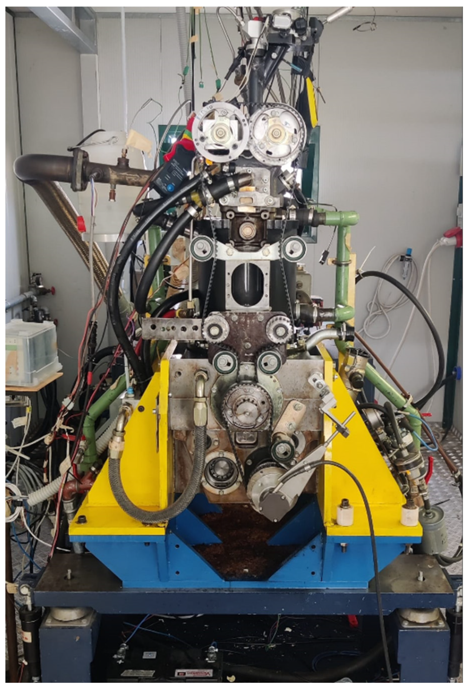
Figure 1. Test engine.
Energies 17 03932 g001
Figure 2. Experimental apparatus.
Energies 17 03932 g002
Figure 3. The trend in the oxygen concentration (O2%) at the exhaust pipe pertaining to an operational case taken as an example, consisting of 100 combustion cycles.
Energies 17 03932 g003
Figure 4. Values of λ for each operating point. The cases highlighted in green were used for training, those in red were used for validation, the cases for which the prediction was made are highlighted in blue.
Energies 17 03932 g004
Figure 5. (a) Overview of the entire dataset including the number of cases analyzed and variables, along with combustion cycles; (b) detailed listing of input and output parameters for each case based on initial sensitivity analysis; (c) division of the dataset into training, testing, and validation sets. Specifically, 80% of the data was allocated to training, 10% to validation, and the remaining 10% to testing for predicting the output variable O2% and deriving the λ value.
Energies 17 03932 g005
Figure 6. The Shapley analysis provides a thorough understanding of the importance of each input feature in predicting the global oxygen concentration. The red line delineates the threshold below which a parameter is deemed insignificant for the purposes of prediction.
Energies 17 03932 g006
Figure 7. (a) Overview of the final dataset including the number of cases analyzed and variables, along with combustion cycles; (b) detailed listing of input and output parameters for each case based on initial sensitivity analysis; (c) division of the dataset into training, testing, and validation sets. Specifically, 80% of the data was allocated to training, 10% to validation, and the remaining 10% to testing for predicting the output variable O2% and deriving the λ value.
Energies 17 03932 g007
Figure 8. (a) Predictive scheme and (b) the internal structure of the LSTM and its division into gates.
Energies 17 03932 g008
Figure 9. The pattern of loss values for the LSTM + 1DCNN architecture, which demonstrated the highest performance during the training session.
Energies 17 03932 g009
Figure 10. Predictions of λ for the three ‘testing cases’ selected by both neural structures: (a) prediction case n.13, (b) prediction case n.21 and (c) prediction case n.38 (refer to Figure 4). The black dotted lines represent the measurement accuracy range of the target, i.e., 0.5%.
Energies 17 03932 g010
Figure 11. Percentage error Err (see Equation (3)) for the three ‘testing cases’ selected and both the BP and LSTM + 1DCNN models, to underline the prediction quality, with the corresponding average percentage error Erravg in the legends. (a) prediction case n.13, (b) prediction case n.21 and (c) prediction case n.38 (refer to Figure 4).
Energies 17 03932 g011
Figure 12. (a) BP regression prediction chart; (b) LSTM + 1DCNN regression prediction chart.
Energies 17 03932 g012aEnergies 17 03932 g012b
Table 1. Engine data [43].
FeatureValueUnit
Displaced volume500cc
Stroke88mm
Bore85mm
Connecting rod length139mm
Compression ratio8.8:1-
Exhaust valve open−13CAD aBDC
Exhaust valve close25CAD aBDC
Intake valve open−20CAD aBDC
Intake valve close−24CAD aBDC
Table 2. Dataset general description and values.
Case
Number
(-)
Combustion
Cycle
(-)
IT
(CAD aTDC)
AI05
(CAD aTDC)
AI50
(CAD aTDC)
AI90
(CAD aTDC)
APmax
(CAD aTDC)
Pmax
(bar)
IMEP
(bar)
ton
(μs)
O2
(%)
11−102.858.7413.5514.0029.073.8519,163.25.892
2−104.6910.6615.2015.9028.073.8219,163.25.886
..........
..........
..........
100−101.166.3210.5211.2031.694.0519,163.25.671
21−101.617.2411.8712.5030.313.9019,163.26.99
2−103.268.4215.0014.0029.483.9719,163.27.02
..........
..........
..........
100−101.627.6012.8112.7029.463.8319,163.25.202
.
.
.
..........
..........
..........
421−19−4.945.9214.0812.402.9123.9614,873.615.130
2−19−5.413.8012.6910.602.7824.5014,873.615.020
..........
..........
..........
100−19−2.487.9016.8613.902.9923.1914,873.614.902
Disclaimer/Publisher’s Note: The statements, opinions and data contained in all publications are solely those of the individual author(s) and contributor(s) and not of MDPI and/or the editor(s). MDPI and/or the editor(s) disclaim responsibility for any injury to people or property resulting from any ideas, methods, instructions or products referred to in the content.