Article

A Bi-Level Reactive Power Optimization for Wind Clusters Integrating the Power Grid While Considering the Reactive Capability

Electric Power Research Institute, State Grid Gansu Electric Power Company, Lanzhou 730070, China
*
Author to whom correspondence should be addressed.
Energies 2024, 17(16), 3910; https://doi.org/10.3390/en17163910
Submission received: 10 July 2024 / Revised: 2 August 2024 / Accepted: 5 August 2024 / Published: 8 August 2024

Abstract

:
With the integration of large-scale wind power clusters into the power system, wind farms play a crucial role in grid reactive power regulation. However, the range of its reactive power remains uncertain, posing challenges in formulating a viable program for regulating reactive power to ensure the safe and cost-effective operation of the power system. Based on this, this paper develops a bi-level reactive power optimization for wind clusters integrating the power grid while considering the reactive capability. Firstly, this paper carries out a refined analysis of the wind power clusters, taking into account the characteristics of different areas to estimate the exact value of the reactive power capability in wind power clusters. Secondly, a bi-level reactive power optimization model is established. The upper-layer optimization aims to minimize active losses and voltage deviation in power system operation, while the lower-layer optimization focuses on maximizing reactive power margin utilization in wind farms. To solve this bi-level optimization model, an improved artificial fish swarm algorithm (AFSA) is employed, which decouples real variables and integer variables to enhance the optimization ability of the algorithm. Finally, the effectiveness of our proposed optimization strategy and algorithm is validated through the simulation results.

1. Introduction

Given the gradual escalation of the energy crisis and increasingly severe environmental problems, achieving sustainable development [1] has emerged as the primary objective for future power grid construction. The low-carbon transformation of energy represents an inevitable global trend in energy development [2], with new energy serving as a crucial prerequisite for driving green and low-carbon advancements and transformations within power systems [3]. However, the large-scale integration of renewable and distributed energy sources poses significant challenges to power grid operation and supervision due to their inherent volatility and unpredictability [4,5].
Reactive power optimization holds paramount importance in the planning, design, and operation of power systems. By effectively optimizing the allocation of reactive power, it enables the precise regulation of voltage levels within the system and mitigates transmission line and transformer losses, thereby enhancing overall system efficiency. Reference [6] proposes an optimization method for day-ahead reactive power planning in order to enhance the voltage safety of the transmission network. This method optimizes the set points for switching shunt, transformer taps, and voltage magnitudes at the regulated buses. The primary objective is to optimize the dynamic reactive power reserve of the system by minimizing the amount of reactive power supplied by synchronous generators. In reference [7], a multi-objective reactive power optimization model is proposed for new energy cluster access to a DC isolated grid, where the objective function includes the active network loss and reactive margin. To solve this multi-objective problem, a weighting method is employed to transform it into a single-objective problem. A novel multi-parameter programming-based distributed algorithm is proposed in reference [8] to solve the coordinated optimal power flow model, which can significantly accelerate the iterative speed between the master and sub-problems.
The existing literature evaluating the reactive power regulation capability of wind farms primarily focuses on the post-evaluation of wind farms’ reactive power regulation capability, as well as the evaluation of their performance under various control strategies. References [9,10] present a methodology for determining the reactive power limit of doubly fed induction generators. It defines the combined reactive power limit of the stator and grid-side converter as the overall reactive power limit of the wind turbine. Additionally, it provides an approach to analyze the reactive power limits of doubly fed wind farms. However, this methodology does not consider the compensating capability of other reactive equipment apart from wind turbines or account for changes in operating conditions within the wind farm. The reactive power regulation capability of wind farms is evaluated in reference [11] using the combination assignment method. This evaluation involves establishing a wind farm model and collecting indicators such as the grid-connected voltage at the field station, the capacity of the reactive power compensation device, and the reactive power margin of the wind turbine. Reference [12] proposes a variable droop control strategy that considers the impact of active wind turbine fluctuations on the reactive power limit of wind farms. This strategy ensures that the reactive power output of wind turbines aligns with the reactive power margin, allowing for an evaluation of both the reactive power regulation capability and voltage at the grid connection point under different control strategies.
To improve the accuracy of reactive power regulation in the actual power system, it is necessary to coordinate the power system and wind power clusters to achieve bi-level optimization. Reference [13] reviews and compares the performance of reactive power dispatch strategies for the loss minimization of doubly fed induction generator-based wind farms. Reference [14] achieves the coordinated control of reactive voltage at multiple time scales for distribution networks with a high proportion of renewable energy sources. Reference [15] proposed a voltage control strategy that coordinates the on-load voltage regulator transformer (OLTC) and reactive power compensation equipment to ensure compliance of the access point voltage with the safe operating range while simultaneously reducing the unit cost. Reference [16] presents a comprehensive approach to reactive power and voltage control, effectively minimizing the frequency of OLTC operations by taking into account the generation and load forecasting. Reference [17] proposes a distributed active and reactive power control strategy based on the multiplier alternating direction method for regional AC transmission systems with wind farms. This strategy aims to optimize power distribution among the wind farms, minimize power loss in the AC transmission system, reduce the deviation of bus voltage from the rated voltage in the wind farm, and minimize power loss in the wind farm collector system. References [18,19] proposed a variable droop control method to assign reactive commands according to the unit reactive margin to improve the utilization of the unit reactive support potential. Reference [20] proposed a multi-objective reactive power optimization control model aiming to enhance the voltage level of wind farms while simultaneously minimizing active losses in collector lines.
Although the aforementioned references have extensively explored the potential of wind power to provide reactive power support, they essentially represent a simple summation of the reactive power limits of each individual unit. The configuration of reactive power capacity in actual wind farms should adhere to the principles of hierarchical and zonal local balancing. However, in numerous engineering practices, more emphasis is placed on the overall configuration rather than consideration of the reactive power zoning within the field. As a result, there is often an occurrence of reactive power flow within the wind farm, leading to additional differential pressure and losses along the transmission lines. Based on this premise, this paper proposes a bi-level strategy for optimizing reactive power in wind power clusters when connecting to the grid while taking into account their inherent potential.
The major contributions of this paper are summarized as follows:
  • A bi-level model is proposed to optimize reactive power and address the integration of large-scale wind power clusters into the power system. To jointly solve the upper and lower layers, a cross-iteration method is employed.
  • The reactive power capacity of the wind power cluster is assessed through meticulous analysis, taking into full consideration the maximum reactive power margin of the wind farm in the optimization strategy to ensure the efficient operation of the power system.
  • An improved artificial fish swarm algorithm is proposed, which decouples real variables and integer variables, reduces the dimensions of variables, enhances the optimization ability of the algorithm, and solves the problem where the algorithm is susceptible to the influence of the local optimum.
The remaining sections of the paper are structured as follows: Section 2 presents a wind cluster topology model. Section 3 conducts a comprehensive analysis of the reactive power capacity within the wind cluster. Section 4 introduces a two-layer optimization model and proposes an enhanced artificial fish swarm algorithm to solve it. In order to evaluate the effectiveness of the proposed two-tier model, arithmetic examples are analyzed in Section 5. Finally, Section 6 provides a summary of this paper.

2. Wind Power Cluster Topology and Reactive Power Analysis

Each wind farm typically consists of multiple lines, with each line being connected to a number of wind turbines. The distance between these units can span hundreds of meters. To establish a representative topology within the wind cluster, as depicted in Figure 1, a total of m lines are interconnected to the low-voltage convergence bus of the wind farm. On each line, n wind turbines are installed and connected to the power system through step-up transformers and outgoing line connections.
During wind farm operation, the power generated by the wind turbines is transmitted through transmission lines and individual transformers. Therefore, it is essential to consider the reactive power losses associated with these transmission components when conducting a detailed analysis of the internal workings of the wind farm.
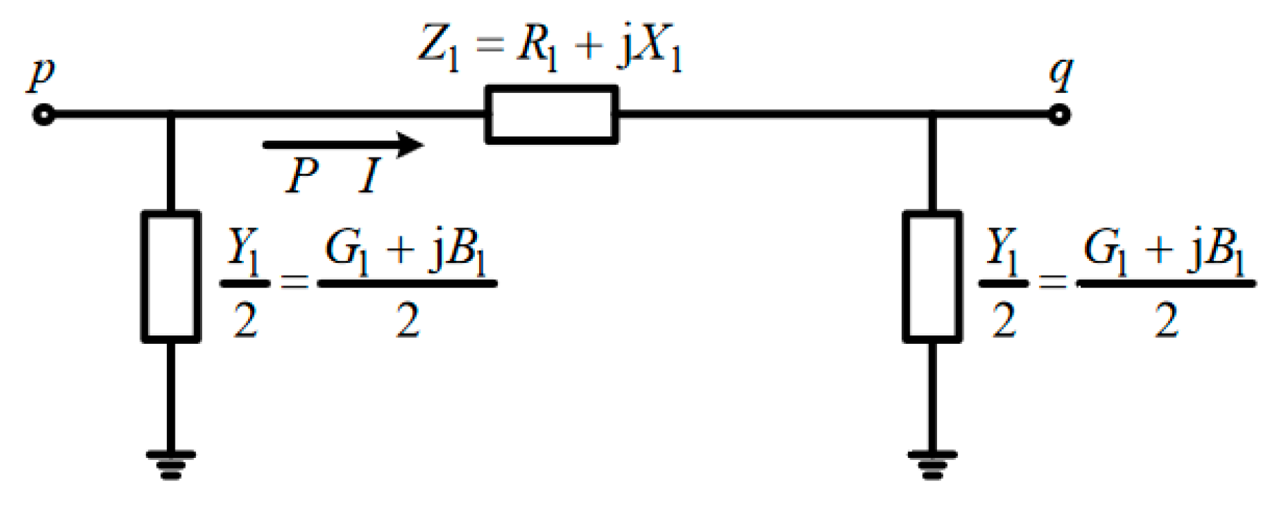
In this case, the π-equivalent circuit of the transmission line is shown in Figure 2.
In order to investigate the correlation between active power and reactive power losses, it is assumed that the system operates under normal conditions with voltage levels approximately being maintained around the per unit value of one. Additionally, it is also assumed that the power factor at the series branch ports is about one, and the mathematical relationship is obtained as follows:
Δ Q Z 1 = I 2 X 1 P = U p I cos φ
Δ Q Z 1 P 2 X 1
where X1 represents the reactance in the line, Y1 represents the admittance in the line, Δ Q Z 1 represents the reactive power consumed by the line impedance, P represents the active power in the line, Up represents the voltage at the beginning of the transmission line, and I represents the current flowing through the line.
The reactive power from the distributed capacitance in the transmission line is:
Q c = B 1 2 U p 2 + B 1 2 U q 2 B 1
Combining the above equations, the reactive power loss of the line can be obtained as:
Q 1 = Δ Q Z 1 Q c P 2 X 1 B 1
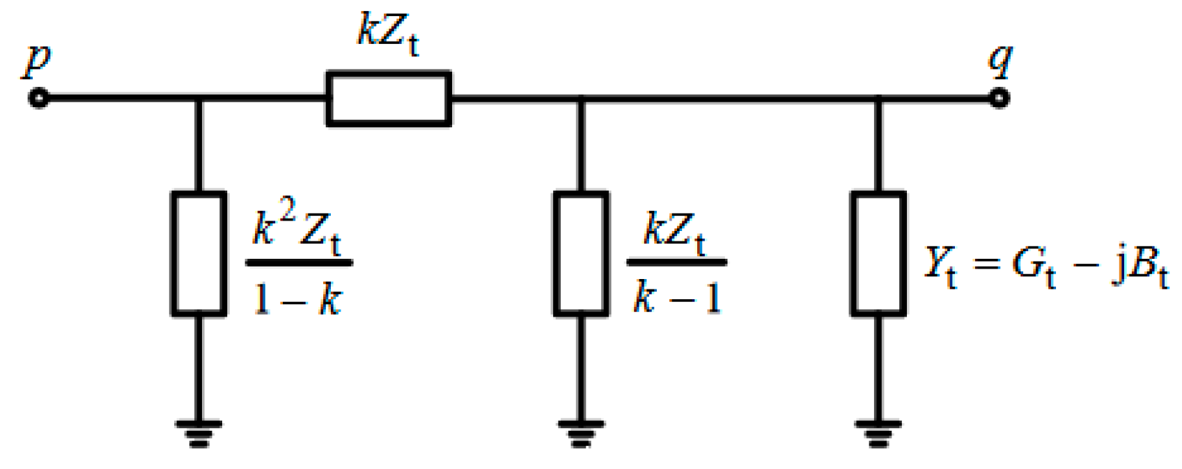
To analyze the transformer reactive power loss, the π-equivalent circuit of the transformer is used as shown in Figure 3:
Zt is the equivalent resistance and leakage reactance of the copper consumption in series with the ideal transformer, k is the non-standard ratio of the transformer using the per-unit value, and Yt is the excitation admittance of its ground branch.
The reactive power loss of the line impedance element in the figure is:
Δ Q Z t = I 2 ( k X t ) P 2 ( k X t )
The sum of the reactive power absorbed by the branch circuits to the ground is:
Q 1 k k 2 X t U p 2 + k 1 k X t U q 2 = 1 k k X t ( U p 2 k U q 2 ) ( 1 k ) 2 k 2 X t
The excitation admittance reactive power loss to the ground is:
Q Y t = B t U q 2 B t
The reactive power loss of the transformer is:
Q t P 2 k X t + ( 1 k ) 2 k 2 X t + B t
A mathematical model of reactive power losses in transmission lines and transformers is proposed based on the current characteristics of collector lines within wind farms to provide a theoretical basis for future research.

3. Wind Cluster Reactive Power Capacity Refinement Analysis

Clustered wind farms consist of interconnected wind turbines, which are linked by collector lines. The reactive power of the wind turbines is transmitted to the power system via long-distance transmission lines, as well as via wind turbine box-type transformers and outgoing channel transformers, resulting in reactive power losses. Simultaneously, the dispersed arrangement of wind turbines within the farm and the intricate voltage distribution internally impacts both operational safety and transmission capacity. Therefore, a refined analysis of reactive power in wind farms is needed.

3.1. Analysis of Wind Turbine Reactive Power Loss

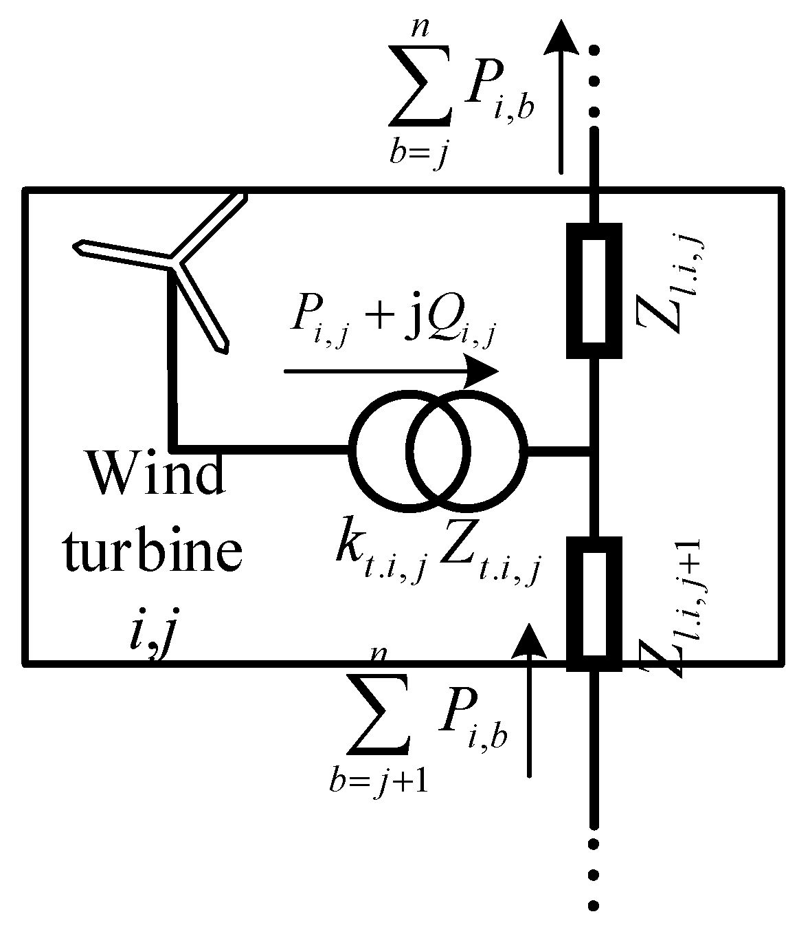
Define the line between turbine j and turbine j − 1 in line i of the wind cluster as ij. The reactive power partition ij centered on the turbine is shown in the Figure 4, which consists of turbine ij, the corresponding box transformer for that turbine, half of the length of transmission line ij, and ij − 1.
The reactive power loss in the upstream transmission line is:
Q l , i , j b = j n P i , b 2 X l . i , j B l . i , j
where Xl,i,j and Bl,i,j represent the reactance and susceptance in the upstream line i,j.
The reactive power loss in the downstream transmission line is:
Q l , i , j + 1 b = j + 1 n P i , b 2 X l . i , j + 1 B l . i , j + 1
where Xl,i,j and Bl,i,j represent the reactance and susceptance in the downstream line i,j + 1.
The reactive power loss of a box transformer connected to an individual wind turbine is:
Q t , i , j P i , j 2 k t . i , j X t . i , j + ( 1 k t . i , j ) 2 k t . i , j 2 X t . i , j + B t . i . j
where Xl,i,j and Bl,i,j represent the reactance and susceptance of the box transformer connected to wind turbine i,j; kt.i,j is the ratio of the box transformer.
The reactive power loss in each turbine region within the wind cluster is thus determined.
Q i , j = 1 2 ( Q l . i , j + Q l . i , j + 1 ) + Q t . i , j

3.2. Analysis of Reactive Power Losses on Converging Lines

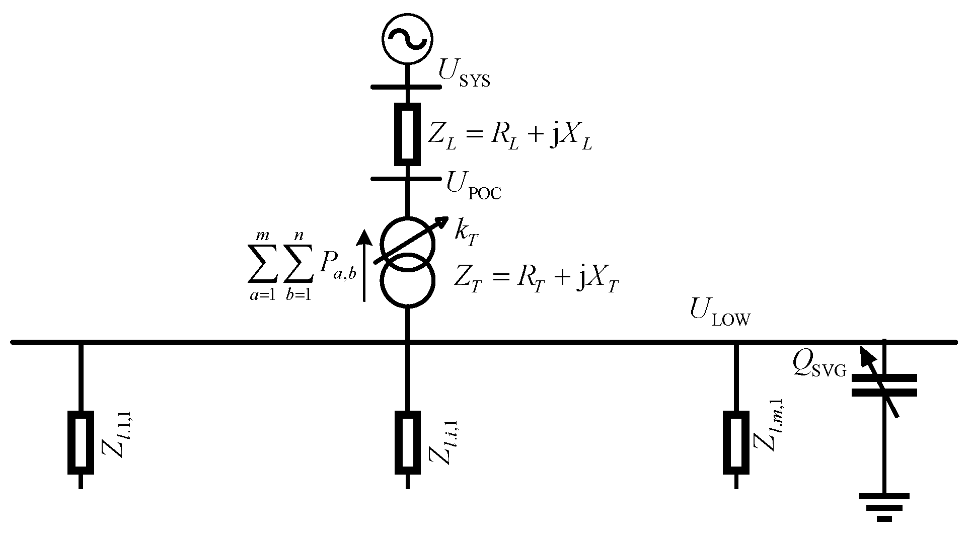
The wind cluster aggregation line topology is shown in the Figure 5, covering the total reactive power with the aggregation station step-up transformer, half of the length of the first section of each line, and the wind cluster aggregation feeder line.
The reactive power loss in the i,1 part of the line is:
Q l , i , 1 b = 1 n P i , b 2 X l . i , 1 B l . i , 1
where Xl,i,1 and Bl,i,1 represent the reactance and susceptance of the first section of the line.
The reactive power loss of the step-up transformer is:
Q T ( a m b n P a , b ) 2 k T X T + ( 1 k T ) 2 k T 2 X T + B T
where XT and BT represent the reactance and susceptance of the step-up transformer in the aggregation line and kT represents the ratio of the step-up transformer.
The reactive power loss on the aggregation line is:
Q L ( a m b n P a , b ) 2 X L B L
where XL and BL are the reactance and susceptance of the aggregation line.
The total reactive power loss of the aggregation line is:
Q S = 1 2 a = 1 m Q l . a , 1 + Q L + Q T

3.3. Total Reactive Power Capacity of Wind Farms

The total reactive power loss of the wind farm is calculated as the sum of the reactive power of each wind turbine corresponding to the region and reactive power of the converging line, and the specific equation is as follows:
Q WT = a = 1 m b = 1 n ( Q l . a , b + Q t . a , b ) + Q L + Q T
In the normal operation of the wind farm, the difference between the total reactive power output of the wind cluster and the total reactive power loss QWT in the wind farm, as calculated by the formula above, represents the effective reactive power capacity of the wind farm.
Q WF = a = 1 m b = 1 n Q wt . a , b Q WT

4. Bi-Level Reactive Power Optimization Model

4.1. Upper-Layer Optimization Model

An hourly optimal model is established in the upper layer, taking into account the impact of large-scale wind power cluster access on the grid’s network loss and voltage, with the objective function of minimizing the active network loss and voltage deviation of the system.
(1)
Objective function
min f 1 = Δ U = i = 1 N U i U i * Δ U i max Δ U i max = U i max U i min
min f 2 = P loss = i , j N c G i j U i 2 + U j 2 2 U i U j cos θ i j
where Ui represents the voltage value of node i in the system; N represents the set of nodes in the system; U i * represents the reference voltage value of node i, which is generally 1.0 p.u.; ΔUimax represents the maximum value of the voltage deviation when node i is safely operated; Ploss represents the total active loss; Ui and Uj represent the voltages of node i and node j, respectively; Gij represents the conductance between nodes i and j; and θij represents the phase difference of voltage between nodes i and j.
(2)
Constraints
Power equation constraints:
P G i P l i = U i j = 1 N U j G i j cos θ i j + B i j sin θ i j Q Gi + Q C i Q l i = U i j = 1 N U j G i j sin θ i j B i j cos θ i j
where PGi represents the active power of the power supply at node i; Pli represents the active power of the load at node i; QGi represents the reactive power of the power supply at node i; Qli represents the reactive power of the load at node i; and QCi represents the reactive output of the reactive compensation device at node i.
Power grid security operational constraints:
U g i min U g i U g i max i N g P g i , min P g i P g i , m ax i N g Q g i , min Q g i Q g i , m ax i N g Q c i , min Q c i Q c i , m ax i N c T k min T k T k max i N t
h m min G i j U i 2 U i U j ( G i j cos θ i j , t + B i j sin θ i j ) h m max
where Ugimax and Ugimin represent the maximum and minimum values of the generator terminal voltage; Pgimax and Pgimin represent the maximum and minimum values of the generator active output; Qgimax and Qgimin represent the maximum and minimum values of the wind turbine reactive output; Qcimax and Qcimin represent the maximum and minimum values of the reactive compensation device cutting capacity; Tkimax and Tkimin represent the maximum and minimum values of the regulator transformer ratios; Ng represents the number of generators; Nc represents the number of reactive power compensation devices; Nt represents the number of regulator transformers; and hm max and hm min represent the maximum and minimum values of branch m-trends.

4.2. Lower-Layer Optimization Model

The lower-layer optimization considers the reactive capability of the wind farm. If only the total reactive power command of the wind cluster is averaged out to each turbine, it is likely to result in the full load of the turbines with smaller reactive power capability and the underutilization of the turbines with larger reactive power capability. Therefore, a 15 min rolling optimization model of wind clusters is established with the objective function of the highest reactive margin utilization of wind clusters at the 15 min level. The active power output value of a cluster of wind turbines is recorded every 15 min, and the reactive power output Qset from the previous 24 intervals is utilized as the initial parameter for optimizing the lower layer. Simultaneously, the optimized wind power output value is employed to update Qgimax and Qgimin as boundaries for subsequent iterations in order to achieve cross-iterative optimization.
(1)
Objective function
The lower-layer optimization model establishes an objective function f3 to quantify the reactive power capacity of wind power. The smaller the value of function f3, the higher the utilization of the reactive power margin in the wind farm. Therefore, the objective function is formulated as follows:
min f 3 ( x ) = i = 1 n ( Q WF i Q WF Q i Q set )
(2)
Constraints
Q WT_min Q WT i Q WT_max P WT_min P WT i P WT_max U i _min U i U i _min
where PWTi and QWTi represent the active and reactive power output of the ith wind turbine, respectively; QWTi_max and QWTi_min represent the upper and lower limits of the wind turbine power output; PWTi_max and PWTi_min represent the upper and lower limits of the wind turbine active power output; and Ui_max and Ui_min represent the upper and lower limits of the voltage at the access point of the ith wind turbine.

4.3. Improved Artificial Fish Schooling Algorithm

The advancement of intelligent optimization algorithms has led to significant progress: multi-objective intelligent optimization methods have emerged, such as the multi-objective genetic algorithm [21,22], multi-objective evolutionary algorithm [23,24], multi-objective differential evolution [25], multi-objective particle swarm optimization (PSO) [26,27], and whale optimization algorithm (WOA) [28].
The PSO approach is an optimization technique proposed to simulate the foraging behavior of a flock of birds by iteratively optimizing the positions of poorly adapted particles. During the optimization process, every particle converges towards both the global optimum within the swarm and its own historical best solution, continuously approaching an improved problem solution. The WOA is an innovative heuristic global optimization algorithm inspired by the hunting behavior of humpback whales. This algorithm effectively explores optimal solutions by mimicking the three key processes employed by humpback whales during their search for prey, namely searching, encircling hunting, and attacking using spiral bubble nets.
However, it should be noted that while searching for the optimal solution, the PSO may encounter local optima resulting in a final outcome that is different from the global optimum. The WOA heavily relies on the quality of its initial solution; thus, if an inadequate initial solution is provided, there is a risk of falling into local optima. Additionally, when confronted with high-dimensional problems, a dimensional catastrophe problem may arise and subsequently hinder the efficiency of this algorithm. To address these drawbacks, this paper proposes an improved artificial fish swarm algorithm.
The AFSA method is a search and optimization technique that incorporates various behaviors observed in fish, such as foraging, aggregation, tailing, and stochastic behavior. It initiates from an individual and employs foraging, swarming, and tail chasing behaviors to explore the global optimum through local optimizations. This approach offers the advantage of rapid convergence compared with traditional algorithms. In most models for reactive power optimization, the number of variables is extensive and encompasses both integer and real variables. The utilization of AFSA for optimization is likely to result in local optimization, as the same number of iterations is applied to both types of variables, significantly prolonging the optimization time.
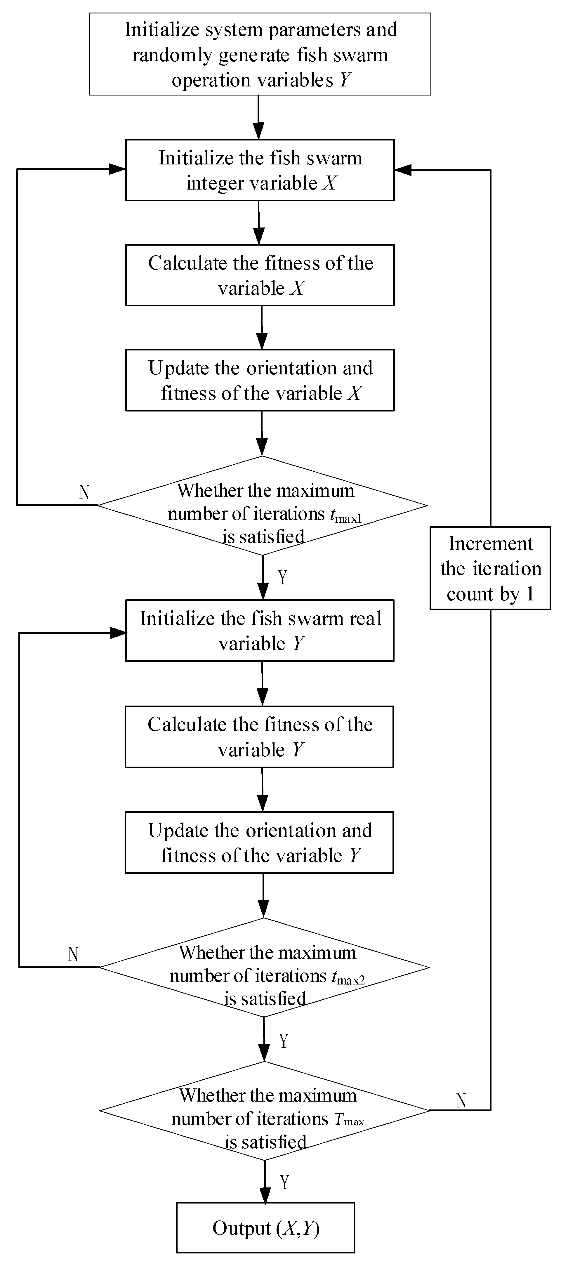
To address this issue, this paper segregates the integer variables X = (X1, X2, …, Xs) and the real variables Y = (Y1, Y2, …, Ys), where s represents the total number of variables. Initially, random generation is employed for obtaining the real variable Y while AFSA optimizes the integer variable X. Because there are fewer combinations involved with integer variables, a reduction in iterations can be appropriately implemented during X optimization. Once optimized quantitative information for X is obtained, it is fed back into variable Y, which undergoes further optimization. Considering that running variables are real and involve more complex combinations of values, an appropriate increase in iterations can be applied during Y optimization. Subsequently, the optimized real variable Y feeds back into integer variable X, which then undergoes its own round of optimization. This process continues iteratively using feedback from each party’s optimized information until reaching satisfaction with Tmax (the maximum number of iterations) within the outer loop. The flowchart of the algorithm is shown in Figure 6, and the specific flow is shown below.
Step 1: Initialization. Input the node and branch information as well as initial data for the power system, and specify parameters including population size (Ns), maximum number of outer loop iterations (Tmax), maximum number of inner loop iterations for the optimized location variable (tmax1), maximum number of inner loop iterations for optimized operation variable (tmax2), range of artificial fish sensing, iteration step, and congestion coefficient α for the improved AFSA.
Step 2: Optimize the individual integer variable X. The individual real variable Y is initialized. The values of each state function of the fish swarm are calculated, and the optimal individual and function values are retained. Subsequently, natural behaviors such as clustering and tail chasing are performed to determine the next swimming direction and update the position of individuals. After tmax1 iterations, the optimal individual position is output.
Step 3: Optimization of the real variable Y. The real variable Y is optimized through AFSA in a similar manner as in step 2, based on the determination of the integer variable X.
Step 4: The number of iterations is incremented by one. The fitness output from step 3 should be retained and compared with the optimal fitness output from the previous step 3. If it is better than the previous optimal fitness, the current state (X, Y) should be kept, and the optimal fitness of this iteration should be updated. When the maximum number of iterations Tmax is reached, proceed to step 5. Otherwise, substitute the output optimal running variable Y into step 2.
Step 5: Output the optimal solution and optimal position.

5. Case Study

5.1. Algorithm Parameter Settings

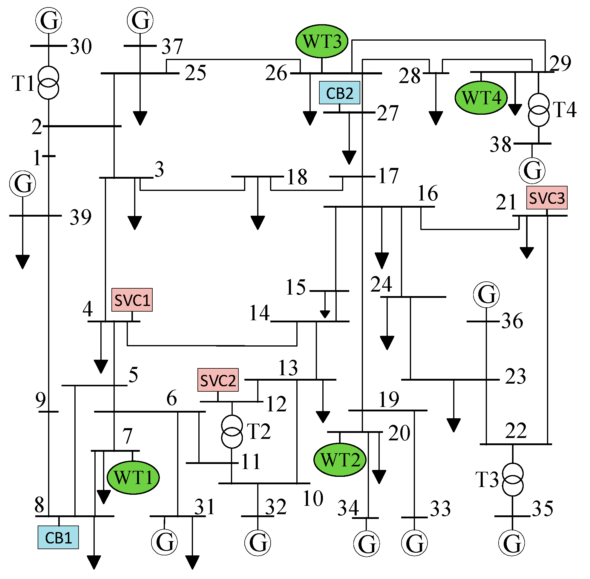
The upper-layer optimization utilizes the improved IEEE-39 node system, as depicted in Figure 7, with a base power of 100 MVA. Wind power clusters WT1, WT2, WT3, and WT4 are connected to nodes 7, 26, 20, and 29, respectively, with a capacity of 45 MW each. OLTCs are configured at lines 2–30, 11–12, 22–35, and 29–3. Capacitor banks (CBs) with a capacity of 20 Mvar are installed at nodes 8 and 27, respectively. Additionally, a static var compensator (SVC) with a capacity of 100 Mvar is connected to nodes 4, 12, and 21. The maximum and minimum values for each variable can be found in Table 1.
The topology of a single line in each wind cluster within the lower optimization model is illustrated in Figure 8. Each feeder comprises ten groups of wind turbines with a rated capacity of 1.875 MW, which are boosted and interconnected to the grid through a high-voltage transmission line.

5.2. Model Verification

To compare the convergence speeds of three different algorithms, Figure 9 illustrates the convergence process of solving a single-objective optimization model for the improved IEEE 39-node system optimal in terms of network loss only. The figure demonstrates that the particle swarm optimization algorithm converges to 106.8 MW after 80 iterations, while the whale optimization algorithm achieves convergence to 110.3 MW after 90 iterations. Moreover, the proposed improved artificial fish swarm optimization algorithm in this study also reaches convergence at 104.2 MW after a mere 60 iterations, showcasing a remarkable enhancement in both convergence speed and optimization capability compared with the other two algorithms.
The figure shows the relationship between the number of solving iterations and active network loss. Compared with using elementary particle swarm and whale algorithms independently, our proposed improved artificial fish swarm optimization algorithm significantly enhances both optimization ability and convergence speed.
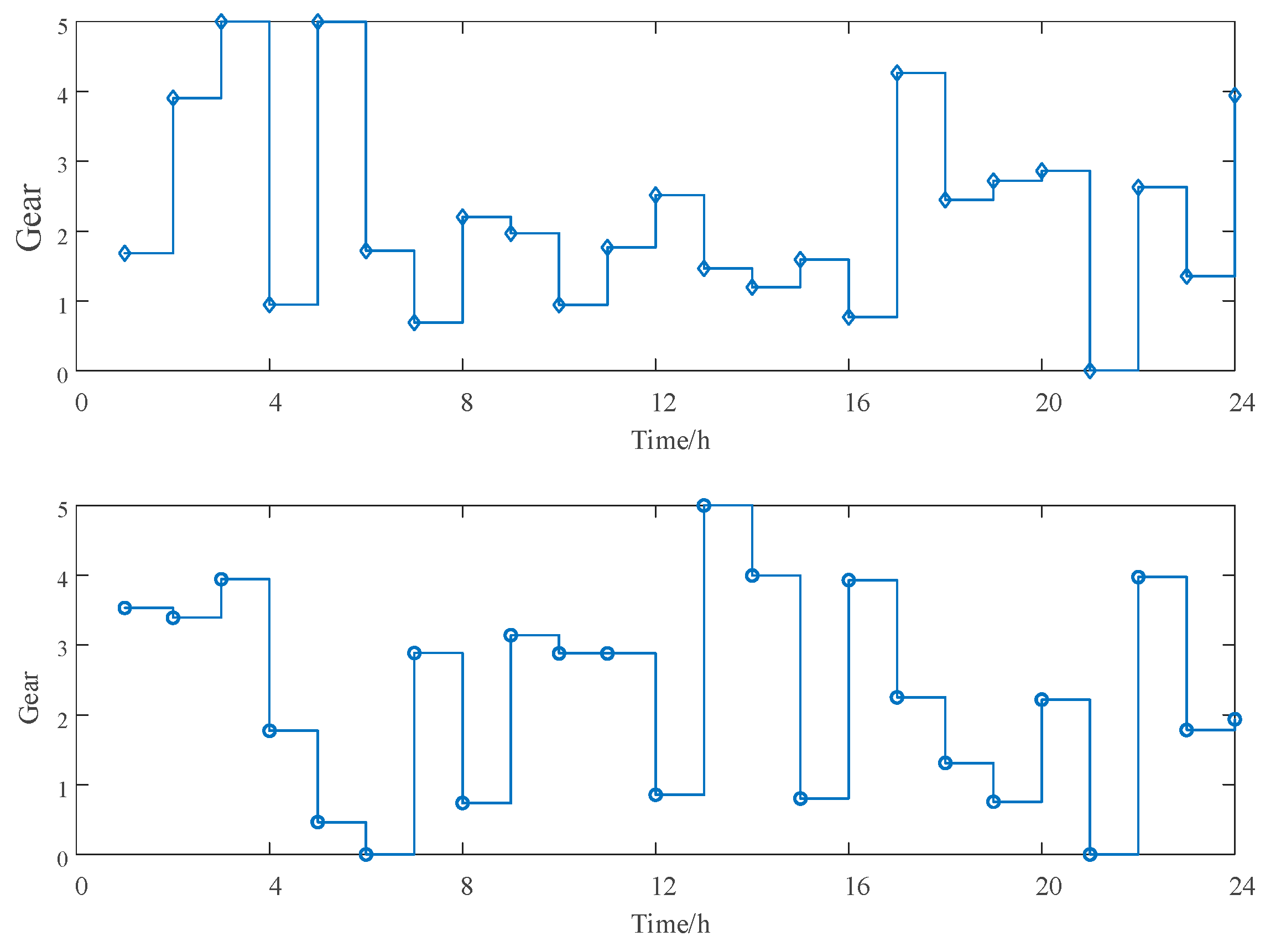
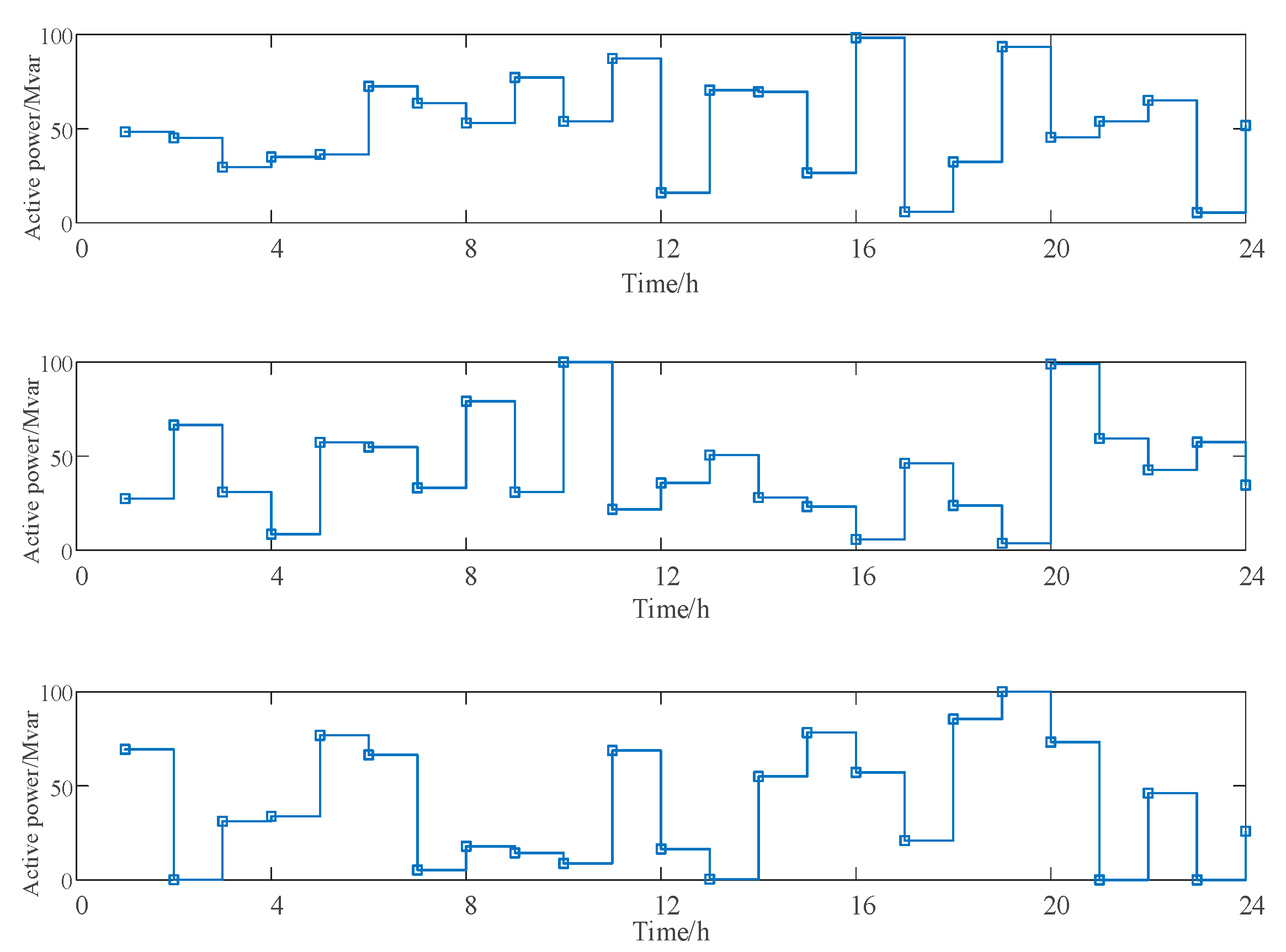
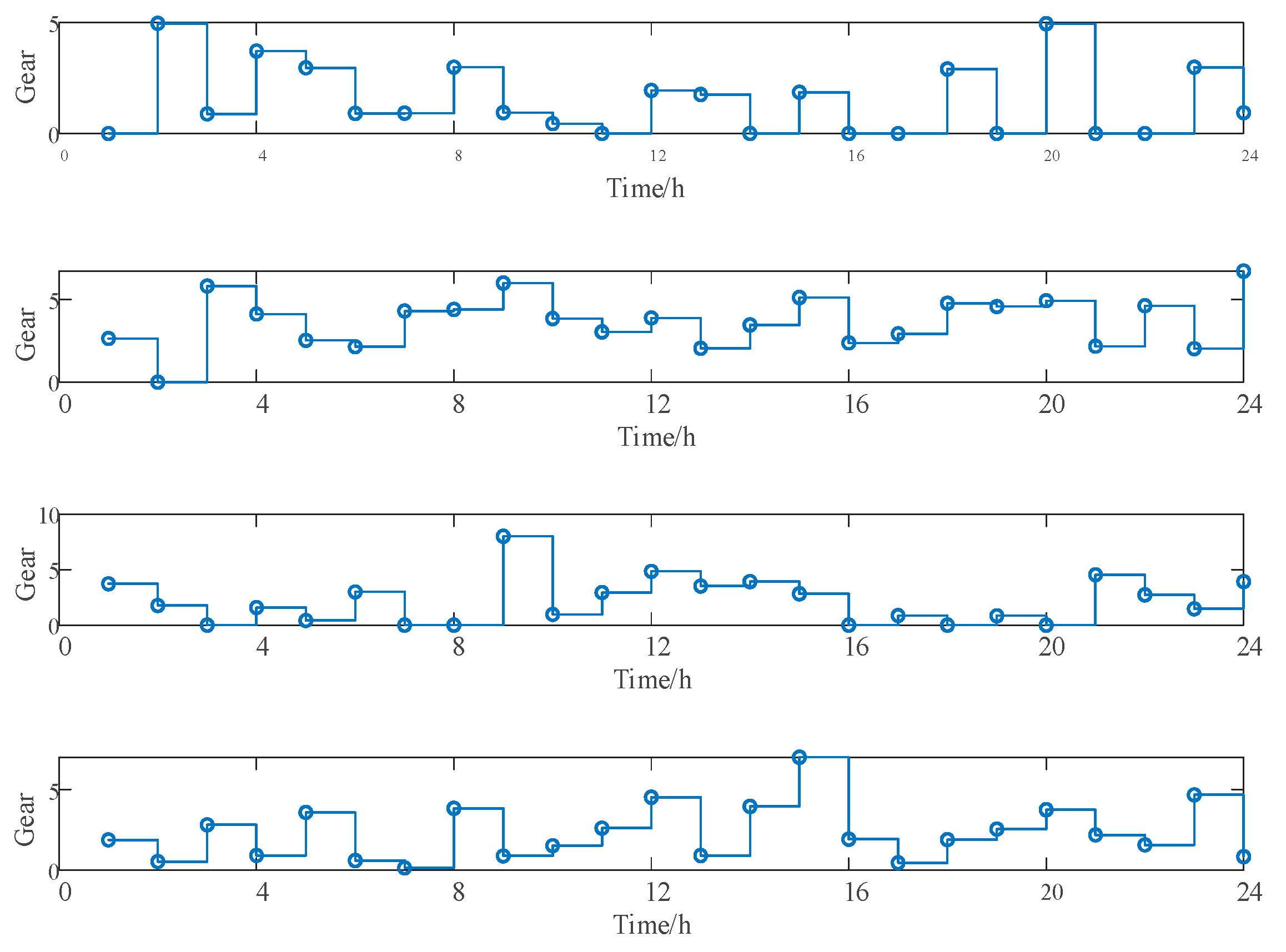
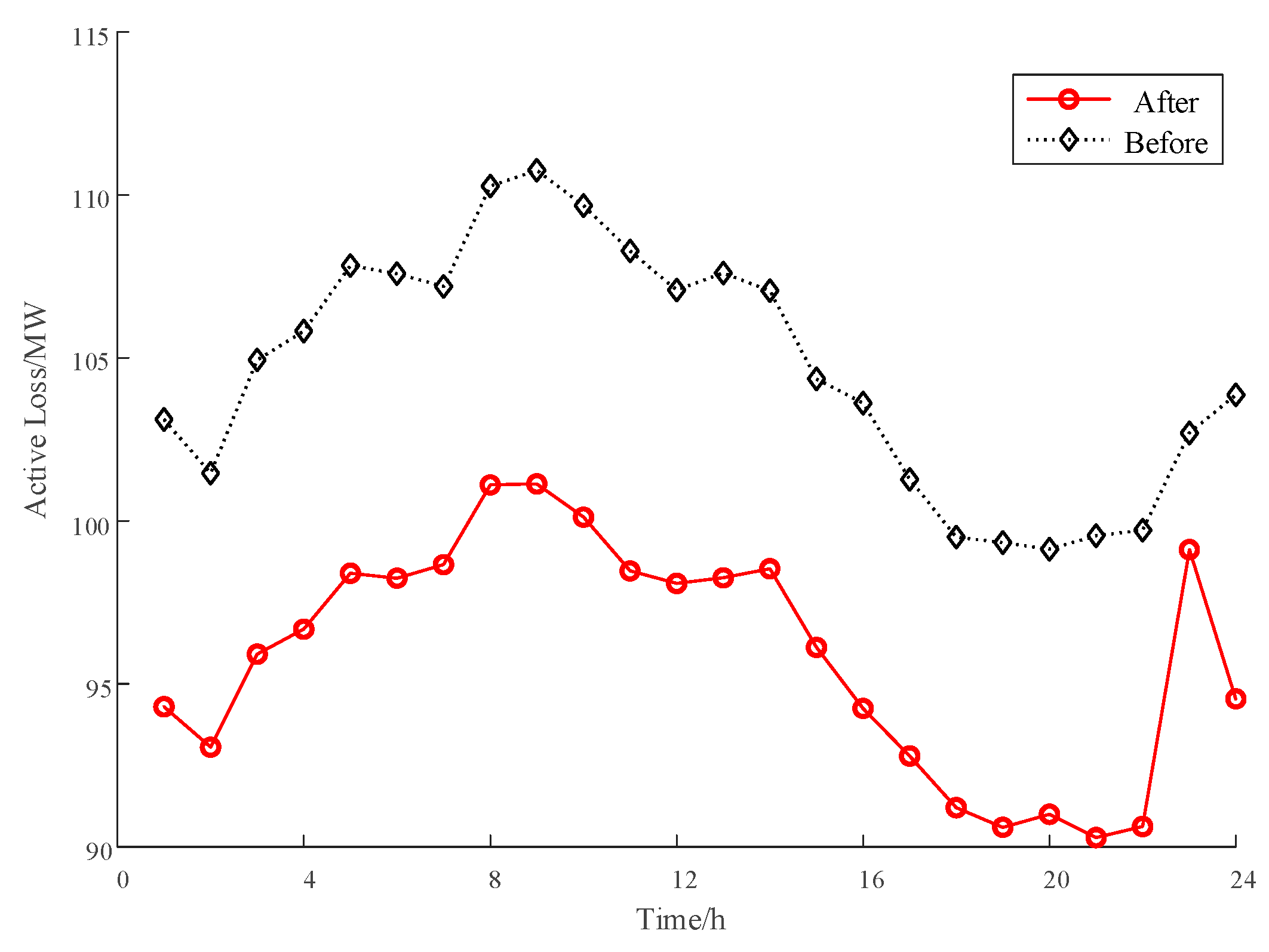
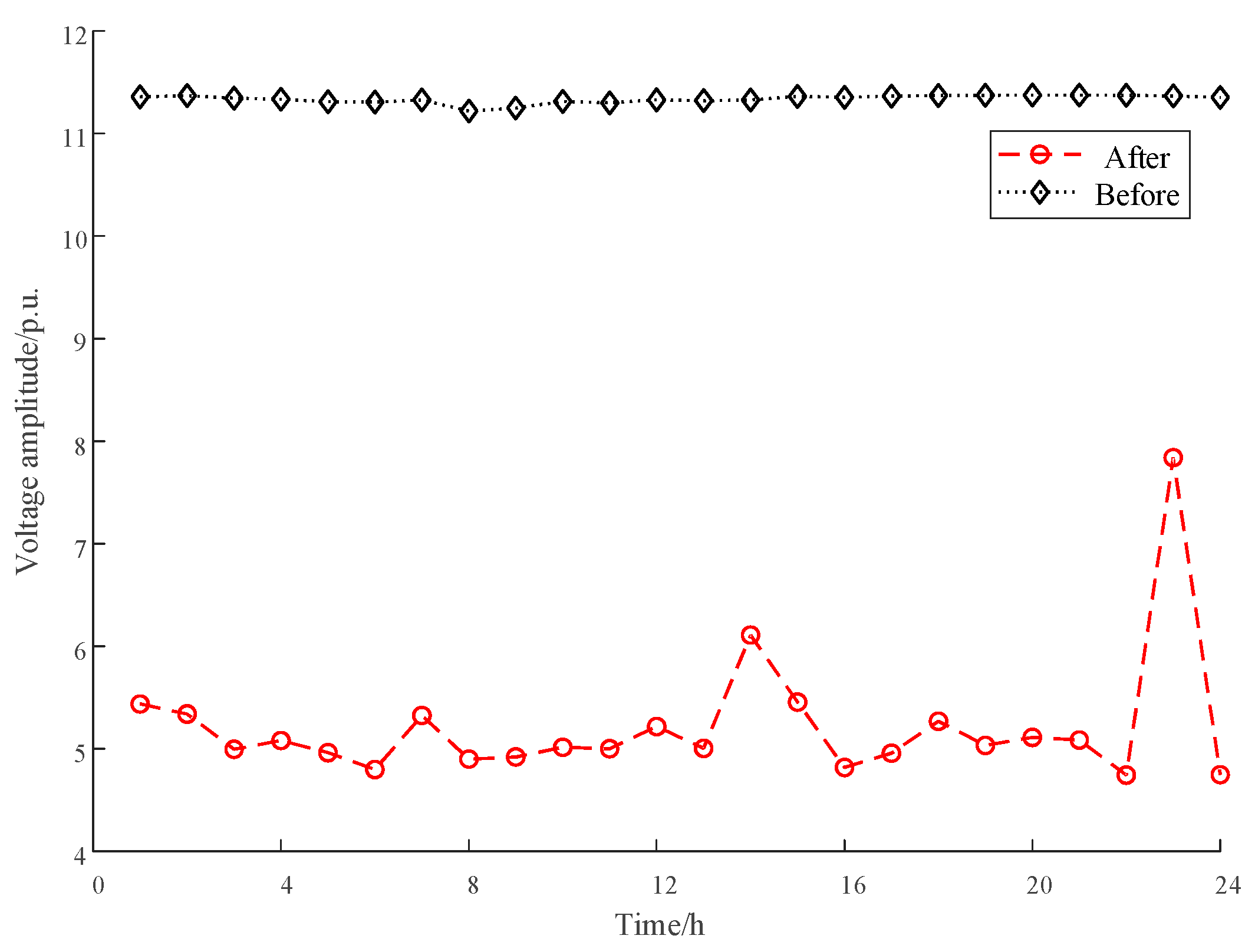
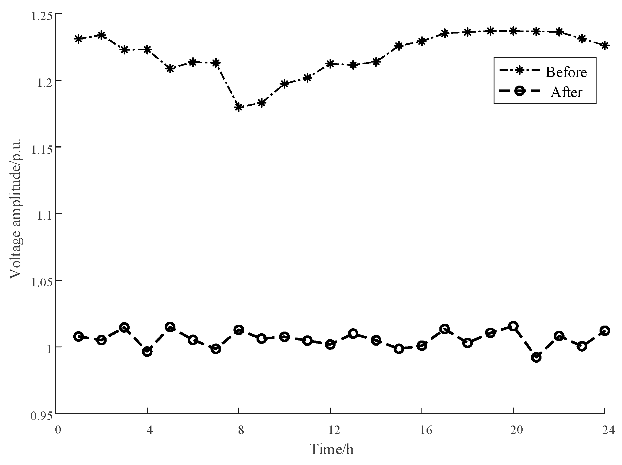
The optimized solution demonstrates the action results of the adjustable reactive devices after undergoing a bi-level optimization, as depicted in Figure 10, Figure 11 and Figure 12. The analysis reveals that the operation of reactive power sources such as CB and SVC complies with the imposed constraints, while the operations of OLTC is also within acceptable adjustable margins. Figure 13, Figure 14 and Figure 15 present a comparison between system network losses, voltage deviation, and voltage amplitude at each node before and after optimization.
In Figure 13, it can be seen that compared with the pre-optimization period, the active losses of the system for 24 moments after using the two-layer reactive power optimization strategy that takes into account the reactive power capability of the wind farm are significantly improved. The average network loss of the grid for 24 h before optimization is 104.6538 MW, and the average voltage deviation is 11.31 p.u. The average network power loss of the system through reactive power optimization is 95.8948 MW, and the average voltage deviation is 5.49 p.u., which is a reduction of loss rate of 8.37%.
The optimization strategy proposed in this paper coordinates the operation of each reactive device in the system while also taking into account the reactive capability of wind power clusters to modify the distribution of reactive current and enhance voltage levels. From Figure 15, it is evident that prior to optimization, there exists a significant voltage amplitude at the wind power access point, which may jeopardize the safe and stable functioning of the system. Through comparative analysis, it can be observed that after optimization, the overall voltage amplitude decreases and stabilizes within an acceptable range throughout all time periods, thereby improving voltage levels.

5.3. Comparative Analysis of Scenarios

The advantages and effectiveness of the bi-level reactive power optimization strategy for wind power cluster access to the grid, considering the reactive power capability of wind farms, are demonstrated through the establishment of three different optimization scenarios and a comparison of the results.
Scenario 1: A single reactive power optimization model, which only considers the impact of reactive power compensation and the regulation of transformer ratios on the system. The impact of the internal structure of the wind cluster and the reactive power capability of the wind farm on the active losses are not considered.
Scenario 2: A single reactive power optimization model, which only considers the influence of the internal structure of the wind cluster and the reactive power capability of the wind farm on active losses. The impact of reactive power compensation and transformer ratio regulation on the system is neglected.
Scenario 3: A bi-level model for reactive power optimization, which examines the impact of reactive power compensation, transformer ratio regulation, the internal structure of wind turbine, and the reactive power capacity of wind farm on active power loss, should be taken into consideration.
The results of the average active power loss for 24 h after an optimization cycle for the three schemes are presented in Table 2. The bi-level optimization strategy is adopted in Scenario 3 to effectively coordinate and optimize the reactive power output of each reactive power source in the power system and each wind turbine in the wind power cluster, resulting in a reduction of network loss value when compared with Scenario 1 and Scenario 2. This comparison demonstrates that our proposed two-layer reactive power optimization approach for wind cluster grid access, which considers the reactive capability of wind farms, yields superior effectiveness in reducing losses.
The active losses of the system after optimization of the three scenarios are compared in Figure 16, revealing that Scenario 1 exhibits the least effective reduction in losses. This can be attributed to its limited regulation capability when integrating large-scale wind power clusters, resulting in difficulties in consuming excess power locally and necessitating the long-distance transmission of surplus active power. Consequently, this leads to in-creased active losses in the transmission lines and a higher value for overall network loss within the system. Scenario 2 solely focuses on optimizing strategies at the wind power cluster level, which only allows for the regulation of active losses through coordination of the reactive power output from wind turbine units without considering reactive power compensation devices at the power system level. As a result, this scenario fails to fully utilize voltage control capability and reactive power regulation capacity. In contrast to these two scenarios, Scenario 3 adopts a bi-level optimization method that coordinates multiple adjustable resources’ support roles regarding reactive power within the power system. By improving both reactive power flow distribution and grid voltage levels while considering the reactive capability of wind clusters, it optimizes their reactive power output and achieves better results in terms of loss reduction compared with other optimization scenarios.

6. Conclusions

In order to address the issue of large-scale wind power cluster connections in power grids, a bi-level reactive power optimization model taking into account the reactive power capability of wind farms is proposed. Initially, a reactive power loss calculation model is established based on the refined analysis of the internal topology of wind power clusters, which are divided into areas centered on wind turbines and areas centered on converging lines. The model takes into account the characteristics of different areas to estimate the exact value of the reactive power capability in wind power clusters. Furthermore, a bi-level reactive power optimization strategy for large-scale wind power clusters accessing the grid is formulated using this method. The upper-layer optimization aims to minimize active losses and voltage deviation in power system operation, while the lower-layer optimization focuses on maximizing reactive power margin utilization in wind farms. Through iterative cross-optimization between these layers, optimal reactive power outputs for each wind turbine unit and each reactive device in the system are determined. Additionally, to solve this bi-level optimization model, an improved AFSA is employed, which decouples real variables and integer variables to enhance the optimization ability of the algorithm.
From the perspective of power grid operation safety and economy, this paper conducts an analysis on the relationship between the active network loss and voltage deviation and the reactive capability of each reactive device and wind power cluster. It establishes a bi-level reactive power optimization model and coordinates both upper layer and lower layer to enhance system stability. This coordination effectively reduces system network losses and voltage deviations, enabling a safe and energy-saving operation of the power grid.

Author Contributions

Conceptualization, X.M.; Methodology, X.M.; Software, W.Z.; Validation, X.M.; Formal analysis, Y.L.; Investigation, R.X.; Resources, X.D.; Data curation, W.Z.; Writing—original draft, W.Z.; Writing—review & editing, Y.L.; Visualization, R.X.; Supervision, X.D. All authors have read and agreed to the published version of the manuscript.

Funding

This research was funded by National Natural Science Foundation of China (NO. 62063015).

Data Availability Statement

The original contributions presented in the study are included in the article, further inquiries can be directed to the corresponding author.

Conflicts of Interest

All authors were employed by the State Grid Gansu Electric Power Company.

References

  1. Zhuo, Z.; Zhang, N.; Hou, Q.; Du, E.; Kang, C. Backcasting Technical and Policy Targets for Constructing Low-Carbon Power Systems. IEEE Trans. Power Syst. 2022, 37, 4896–4911. [Google Scholar] [CrossRef]
  2. Jin, H.; Guo, J.; Tang, L.; Du, P. Long-Term Electricity Demand Forecasting under Low-Carbon Energy Transition: Based on the Bidirectional Feedback between Power Demand and Generation Mix. Energy 2024, 286, 129435. [Google Scholar] [CrossRef]
  3. Guţu-Chetruşca, C.; Braga, D. Energy Crises—Energy Transition Driving Force. In Proceedings of the 2023 International Conference on Electromechanical and Energy Systems (SIELMEN), Craiova, Romania, 11–13 October 2023; pp. 1–6. [Google Scholar]
  4. Ouyang, J.; Li, M.; Diao, Y.; Tang, T.; Xie, Q. Active Control Method of Large-Scale Wind Integrated Power System with Enhanced Reactive Power Support for Wind Speed Fluctuation. IET Gener. Transm. Distrib. 2018, 12, 5664–5671. [Google Scholar] [CrossRef]
  5. Zeng, L.; Chiang, H.-D. Online and Look-Ahead Determination of the Renewable Admissible Region for Managing the Uncertainty of Renewables: Theory and Some Applications. IEEE Trans. Power Syst. 2024, 39, 5609–5619. [Google Scholar] [CrossRef]
  6. Ibrahim, T.; Rubira, T.T.D.; Rosso, A.D.; Patel, M.; Guggilam, S.; Mohamed, A.A. Alternating Optimization Approach for Voltage-Secure Multi-Period Optimal Reactive Power Dispatch. IEEE Trans. Power Syst. 2022, 37, 3805–3816. [Google Scholar] [CrossRef]
  7. Yin, S.; Wu, L.; Song, W.; Wang, X. Multi-Objective Reactive Power Optimisation Approach for the Isolated Grid of New Energy Clusters Connected to VSC-HVDC. In Proceedings of the 6th International Conference on Renewable Power Generation, Wuhan, China, 19–20 October 2017; Institution of Engineering and Technology: Beijing, China, 2017; Volume 2017, pp. 1024–1028. [Google Scholar]
  8. Yang, M.; Liu, Y.; Guo, L.; Wang, Z.; Zhu, J.; Zhang, Y.; Cheng, B.; Wang, C. Hierarchical Distributed Chance-Constrained Voltage Control for HV and MV DNs Based on Nonlinearity-Adaptive Data-Driven Method. IEEE Trans. Power Syst. 2024, 1–14. [Google Scholar] [CrossRef]
  9. Lopez, J.; Gubia, E.; Olea, E.; Ruiz, J.; Marroyo, L. Ride Through of Wind Turbines With Doubly Fed Induction Generator Under Symmetrical Voltage Dips. IEEE Trans. Ind. Electron. 2009, 56, 4246–4254. [Google Scholar] [CrossRef]
  10. Zou, X.; Zhu, D.; Hu, J.; Zhou, S.; Kang, Y. Mechanism Analysis of the Required Rotor Current and Voltage for DFIG-Based WTs to Ride-Through Severe Symmetrical Grid Faults. IEEE Trans. Power Electron. 2018, 33, 7300–7304. [Google Scholar] [CrossRef]
  11. Shen, Y.; Zu, W.; Liang, L.; Zhang, B.; Li, Y.; Peng, Y. Comprehensive Evaluation of the Reactive Power and Voltage Control Capability of a Wind Farm Based on a Combined Weighting Method. Dianli Xitong Baohu Yu Kongzhi/Power Syst. Prot. Control 2020, 48, 18–24. [Google Scholar] [CrossRef]
  12. Li, Y.; Xu, Z.; Zhang, J.; Meng, K. Variable Droop Voltage Control For Wind FarmVariable Droop Voltage Control For Wind Farm. IEEE Trans. Sustain. Energy 2018, 9, 491–493. [Google Scholar] [CrossRef]
  13. Zhang, B.; Hu, W.; Hou, P.; Tan, J.; Soltani, M.; Chen, Z. Review of Reactive Power Dispatch Strategies for Loss Minimization in a DFIG-Based Wind Farm. Energies 2017, 10, 856. [Google Scholar] [CrossRef]
  14. Xu, Y.; Dong, Z.Y.; Zhang, R.; Hill, D.J. Multi-Timescale Coordinated Voltage/Var Control of High Renewable-Penetrated Distribution Systems. IEEE Trans. Power Syst. 2017, 32, 4398–4408. [Google Scholar] [CrossRef]
  15. von Appen, J.; Stetz, T.; Braun, M.; Schmiegel, A. Local Voltage Control Strategies for PV Storage Systems in Distribution Grids. IEEE Trans. Smart Grid 2014, 5, 1002–1009. [Google Scholar] [CrossRef]
  16. Agalgaonkar, Y.P.; Pal, B.C.; Jabr, R.A. Distribution Voltage Control Considering the Impact of PV Generation on Tap Changers and Autonomous Regulators. IEEE Trans. Power Syst. 2014, 29, 182–192. [Google Scholar] [CrossRef]
  17. Wang, P.; Wu, Q.; Huang, S.; Li, C.; Zhou, B. ADMM-Based Distributed Active and Reactive Power Control for Regional AC Power Grid with Wind Farms. J. Mod. Power Syst. Clean Energy 2022, 10, 588–596. [Google Scholar] [CrossRef]
  18. Kim, J.; Seok, J.-K.; Muljadi, E.; Kang, Y.C. Adaptive Q–V Scheme for the Voltage Control of a DFIG-Based Wind Power Plant. IEEE Trans. Power Electron. 2016, 31, 3586–3599. [Google Scholar] [CrossRef]
  19. Kim, J.; Muljadi, E.; Park, J.-W.; Kang, Y.C. Flexible IQ–V Scheme of a DFIG for Rapid Voltage Regulation of a Wind Power Plant. IEEE Trans. Ind. Electron. 2017, 64, 8832–8842. [Google Scholar] [CrossRef]
  20. Ren, X.; Wang, H.; Wang, Z.; Wang, Q.; Li, B.; Wu, H.; Yang, J.; Wang, W. Reactive Voltage Control of Wind Farm Based on Tabu Algorithm. Front. Energy Res. 2022, 10, 902623. [Google Scholar] [CrossRef]
  21. Deb, K.; Pratap, A.; Agarwal, S.; Meyarivan, T. A Fast and Elitist Multiobjective Genetic Algorithm: NSGA-II. IEEE Trans. Evol. Comput. 2002, 6, 182–197. [Google Scholar] [CrossRef]
  22. Yan, W.; Liu, F.; Chung, C.Y.; Wong, K.P. A Hybrid Genetic Algorithm–Interior Point Method for Optimal Reactive Power Flow. IEEE Trans. Power Syst. 2006, 21, 1163–1169. [Google Scholar] [CrossRef]
  23. Jayabarathi, T.; Jayaprakash, K.; Jeyakumar, D.N.; Raghunathan, T. Evolutionary Programming Techniques for Different Kinds of Economic Dispatch Problems. Electr. Power Syst. Res. 2005, 73, 169–176. [Google Scholar] [CrossRef]
  24. Ghasemi, M.; Aghaei, J.; Akbari, E.; Ghavidel, S.; Li, L. A Differential Evolution Particle Swarm Optimizer for Various Types of Multi-Area Economic Dispatch Problems. Energy 2016, 107, 182–195. [Google Scholar] [CrossRef]
  25. Li, R.; Yang, Y. Multi-Objective Capacity Optimization of a Hybrid Energy System in Two-Stage Stochastic Programming Framework. Energy Rep. 2021, 7, 1837–1846. [Google Scholar] [CrossRef]
  26. Koad, R.B.A.; Zobaa, A.F.; El-Shahat, A. A Novel MPPT Algorithm Based on Particle Swarm Optimization for Photovoltaic Systems. IEEE Trans. Sustain. Energy 2017, 8, 468–476. [Google Scholar] [CrossRef]
  27. Hou, P.; Chen, Z. Optimized Placement of Wind Turbines in Large-Scale Offshore Wind Farm Using Particle Swarm Optimization Algorithm. IEEE Trans. Sustain. Energy 2015, 6, 1272–1282. [Google Scholar] [CrossRef]
  28. Ahmed, I.; Alvi, U.-E.-H.; Basit, A.; Rehan, M.; Hong, K.-S. Multi-Objective Whale Optimization Approach for Cost and Emissions Scheduling of Thermal Plants in Energy Hubs. Energy Rep. 2022, 8, 9158–9174. [Google Scholar] [CrossRef]
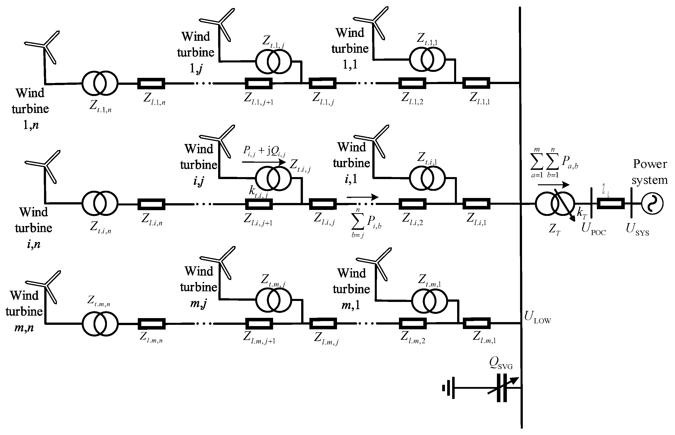
Figure 1. The topological diagram of the wind power cluster.
Energies 17 03910 g001
Figure 2. Transmission line structure diagram.
Energies 17 03910 g002
Figure 3. Transformer equivalent structure diagram.
Energies 17 03910 g003
Figure 4. Reactive power partition diagram centered on the wind turbine.
Energies 17 03910 g004
Figure 5. Reactive power partition diagram centered on the convergence line.
Energies 17 03910 g005
Figure 6. Specific process of the improved artificial fish swarm algorithm.
Energies 17 03910 g006
Figure 7. Improved IEEE-39 node system architecture.
Energies 17 03910 g007
Figure 8. Simplified topology diagram of the lower layer.
Energies 17 03910 g008
Figure 9. Convergence curves for different algorithms.
Energies 17 03910 g009
Figure 10. CB operation logic.
Energies 17 03910 g010
Figure 11. SVC operation logic.
Energies 17 03910 g011
Figure 12. OLTC operation logic.
Energies 17 03910 g012
Figure 13. Active loss comparison diagram.
Energies 17 03910 g013
Figure 14. Voltage deviation comparison diagram.
Energies 17 03910 g014
Figure 15. Voltage comparison diagram of the access point in the wind power cluster.
Energies 17 03910 g015
Figure 16. Comparison diagram of the active power loss after the optimization of each scenario.
Energies 17 03910 g016
Table 1. Maximum and minimum values of each variable.
Controllable VariableMaximum ValuesMinimum Value
Tk/p.u.1.10.9
QCB/group50
QSVC/Mvar1000
α188
γ2515
Table 2. Optimization results of each scenario.
ScenarioActive Power Loss/MW
Scenario 1107.4
Scenario 2104.9
Scenario 395.4
Disclaimer/Publisher’s Note: The statements, opinions and data contained in all publications are solely those of the individual author(s) and contributor(s) and not of MDPI and/or the editor(s). MDPI and/or the editor(s) disclaim responsibility for any injury to people or property resulting from any ideas, methods, instructions or products referred to in the content.