1. Introduction
Power generation and distribution have undergone significant development over the past decade [
1]. Faced with the depletion of fossil energy around the world and the urgent need for global net zero CO
2 emissions, the large-scale development of green renewable energy has become an important way to improve the energy structure and achieve sustainable economic and social development. On the one hand, the increasing popularity of renewable energy can allow an entire power system to run at low cost while generating low pollution. On the other hand, the variable nature of renewable energy, the prediction error of power generation and the significant uncertainty of the load demands limit the applications of renewable energy and present important challenges to the reliability of the system. Therefore, considering the relevant uncertainty in power system scheduling is an important measure to ensure the safety and stability of a power system.
Wind power is the fastest-growing renewable energy source in the world [
2]. However, wind power exhibits great randomness and fluctuations, so the uncertain scheduling of power systems that include wind power is an important research direction.
Depending on how the uncertain factors are modelled, methods of uncertain scheduling involving wind power can be divided into stochastic programming (SP) methods [
3,
4] and robust optimization (RO) methods [
5,
6]. In practical applications, both methods have certain disadvantages. Scenario-based SP has poor out-of-sample performance unless the number of scenarios is very large, which in turn increases the computational burden [
7]. RO provides a conservative solution for a given set of uncertainties, but it is challenging to describe all potential distributions with a single set of uncertainties [
8].
Delage et al. [
9] proposed a model for describing uncertainties in distributional and instantaneous information called distributionally robust optimization (DRO). It is able to incorporate an entire family of potential uncertainty distributions into a problem and solve it in a computationally tractable manner, with both randomness and robustness in the constraints. The establishment of fuzzy sets is an important step in DRO.
Chen et al. [
10] proposed a distance-based distributed robust unit combination model. The fuzzy sets in this model are formed on the basis of the Kullback–Leibler (KL) divergence. In [
11], a distributed robust approximation framework based on the Wasserstein metric was applied to unit allocation problems to manage the risk of uncertain wind power generation prediction errors. The proposed framework minimizes the generating cost, start-up cost, shut-down cost, reserve cost, and the expected thermal generation adjusting cost under the worst-case distribution in the ambiguity set. In addition, some researchers have constructed fuzzy sets from the first or second moments of uncertain variables [
12,
13].
Solving a DRO problem requires a mathematical transformation of the original problem [
14]. In fact, several mathematical optimization methods have been applied to implement the economic scheduling of power systems successfully, including the Newton method, the generalized gradient descent method, the simplex method, the Lagrangian Relaxation method and the interior point method [
15,
16,
17]. However, the optimization performance of the mathematical solution is poor for non-convex problems, and these methods are not suitable for multi-objective problems.
In recent years, with the development of intelligent solution technology, metaheuristic algorithms have been applied for the uncertain scheduling of power systems [
18]. In [
19], the variable characteristics of wind speed and power demand were considered simultaneously, fuzzy logic and dynamic cost coefficients were introduced into the objective function, and a Genetic Algorithm (GA) was used to solve the proposed economic scheduling model to obtain the optimal power generation cost. In [
20], an optimal scheduling model considering the uncertainty of wind power prediction was constructed based on a comprehensive formula for different operation constraints, and a two-step method combining an improved Bat Algorithm (BA) and fuzzy set theory was adopted to solve the multi-objective optimal scheduling problem. Zhang et al. [
21] proposed an improved Differential Evolution (DE) algorithm to solve the optimal scheduling problem in terms of economic emissions, taking into account the non-convex, stochastic and complex-coupled constrained characteristics of hybrid energy systems including wind power and photovoltaic power generation. In [
22], considering the influence of uncertain factors such as renewable energy fluctuations, load fluctuation errors and unit failure and shutdown, an improved Particle Swarm Optimization (PSO) algorithm combined with Monte Carlo simulation was adopted to solve the objective function. In addition, other meta-heuristic methods used for uncertain power system scheduling include: the Cuckoo Search (CS) algorithm [
23], Firefly Algorithm (FA) [
24], and Ant Colony Optimization (ACO) algorithm [
25]. Nevertheless, although the above algorithms can be used to realize uncertain economic scheduling, there is little research on the use of metaheuristic algorithms to solve distributed robust scheduling problems.
Most optimal scheduling methods with wind power uncertainty only consider the uncertainty of wind power output when modelling, and there is a lack of joint modelling research on power load demand and wind power output uncertainty. In addition, the construction and optimization of uncertain sets also need further improvement.
At present, the optimal scheduling model established by the distributionally Robust Optimization method is basically solved by mathematical methods after transformation due to the nature of fuzzy sets. However, due to the limitations of mathematical methods, the results of scheduling problems considering uncertainty are affected to some extent. When the meta-heuristic method is used to solve the optimal scheduling model, there is a lack of research on the adjustment optimization of the relevant uncertainty set, the transformation of the objective function and constraint conditions, and the meta-heuristic solution methods.
Aiming at the construction of uncertain sets, the establishment of a DRO scheduling model, and the problems encountered in model transformation and solving, this paper proposes an uncertain power system scheduling model based on an improved DE algorithm. The main contributions of this paper are as follows:
By analysing the differences in load prediction errors and wind power prediction errors, different types of fuzzy sets are established accordingly.
Based on the DRO algorithm, an uncertain scheduling model is established for a hybrid power system, including thermal power and wind power.
The scheduling model is transformed into a solvable linear programming problem by using a data-driven method and Conditional Value at Risk (CVaR) approximation.
A hybrid solution method based on the simplex method and an improved DE algorithm is proposed. The feasibility of this method is proven based on the IEEE 6-Bus system.
The rest of this paper is organized as follows: In
Section 2, the Wasserstein metric is briefly introduced, and the fuzzy sets of load demand and wind power generation error are constructed. In
Section 3, a distributed robust chance-constrained scheduling model including thermal power generation and wind power generation is established, and the problem is transformed into a solvable linear programming problem. In
Section 4, the hybrid scheduling model based on the simplex method and an improved DE algorithm is described in detail.
Section 5 presents some experimental studies and a discussion of their results. In
Section 6, the conclusions of this study are given, and future research plans are discussed.
2. Fuzzy Sets of Power Load and Wind Power Based on the Wasserstein Distance
2.1. Wasserstein Distance
A probability distance metric can be obtained based on the concept of a probability measure. For a given probability space (Ω,
F,
), Ω represents the sample space, and
F is the
σ-algebra in Ω that defines the measurable set. Suppose that different random events constitute n event subsets
Ei (
i = 1, 2 …
n); then,
F can also be regarded as a set of event subsets
Ei in Ω.
represents the probability distribution, which is used to describe the probability rule for an event occurring in a random experiment. The probability distribution measure satisfies the following conditions:
Therefore, every probability space has a measure that takes a value of 1 for the whole space, and the probability measures of all subsets fall into the unit interval [0,1].
Let two random variables
ξ1 and
ξ2 be defined, which induce two probability distributions
and
, respectively. The probability distance defines the distance between these two probability distribution measures [
26]. To evaluate the distance between the two distributions
and
, the Wasserstein distance
dw is expressed as:
where Ξ
2 represents the supporting spaces of the random variables, Π represents the joint probability distribution of the random variables
ξ1 and
ξ2 in terms of any norm, and
and
are the marginal distributions of the two random variables. Moreover, inf represents the greatest lower bound; that is, the lower bound that can be obtained based on the integral value for all possible joint probability density distributions is the Wasserstein distance.
The fuzzy set formed based on the Wasserstein distance can be expressed as:
where
represents the empirical distribution and
wd is a non-negative parameter that limits the distance between a distribution in the fuzzy set and the empirical distribution.
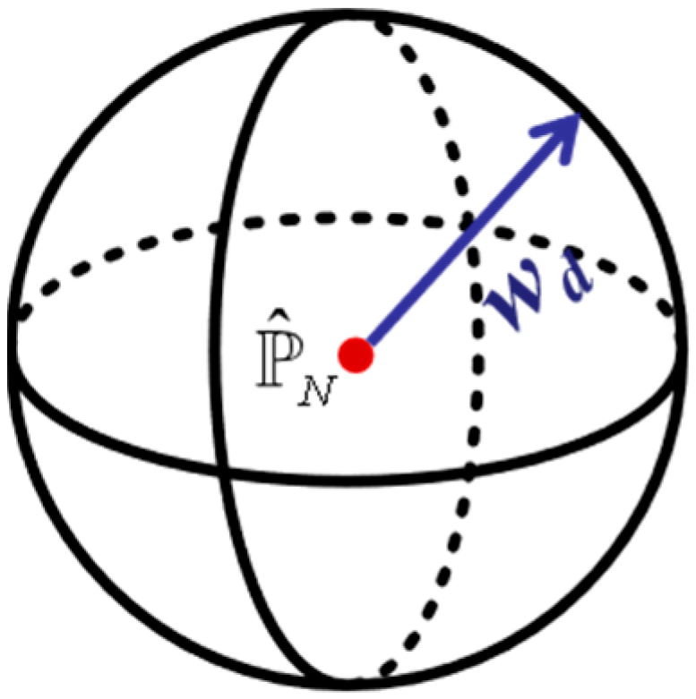
As shown in
Figure 1, the fuzzy set based on the Wasserstein distance is equivalent to the Wasserstein ball with the empirical distribution at the centre and a radius of
wd.
The distributions within the Wasserstein fuzzy set can be viewed as those that pass the multivariate goodness-of-fit test according to the available training samples. This is equivalent to interpreting the Wasserstein distance between the empirical distribution and a given hypothesis distribution as a test statistic and the radius of the Wasserstein fuzzy set as a threshold to be selected based on the level of significance required for the test.
2.2. Uncertainty of Power Load Demand
The uncertainty of the power load demand is mainly reflected in the randomness of the prediction errors obtained by different models. Although the power loads in different seasons and months exhibit certain differences in value, the variation trends of the daily load curves show high similarity. Therefore, for the same model, the load prediction error in a specific period will be similar. Since the prediction error has all of the attributes of a one-dimensional random variable, it can be represented by a probability distribution representing the variation in value of a random variable. According to statistical principles, the probability distribution function of a random variable can be fitted based on the mean value, standard deviation, kurtosis and skewness of the distribution.
In order to achieve the expressibility of random error variables, a special probability distribution can be used for simplification and approximation [
27]. The standard deviation of the normal distribution is 1, the skewness is 0, and the kurtosis is 3, so the basic statistics of the load prediction error are close to the normal distribution numerically. In this paper, a normal distribution test was established to determine whether the distribution of the random variable follows the normal distribution. Under the premise that the number of samples is greater than 30, whether the Jarque–Bera statistic obeys the chi-square distribution with 2 degrees of freedom determines whether the probability distribution of this random variable is normal, which is specifically expressed as:
where
N is the sample size and
c and
α are the skewness and kurtosis of the random variables, respectively.
For the data set adopted in this paper, load prediction was carried out first, and various statistical values of random variables of load prediction error were calculated, as shown in
Table 1.
By calculating the Jarque–Bera statistics and hypothesis testing results, it is proven that the probability distribution of the load prediction error follows a normal distribution, and it can be expressed as:
The load power error value Δ
PL associated with the probability of load power fluctuation is obtained by means of the inverse of the cumulative distribution function:
For a normal distribution, the probability range can be expressed in the form of a confidence interval. Thus, the fuzzy set of the power load demand can be expressed in interval form as follows:
where
PL,t represents the load power of the uncertain factor at time
t;
αt represents the significance level of the normal distribution; and
and
represent the upper and lower limits, respectively, on the load fluctuation at a certain time.
2.3. Uncertainty of Wind Power Output
The uncertainty of wind power output is more difficult to describe than the uncertainty of load prediction. The output power of a wind turbine has a complex physical relationship with the wind speed, temperature and wind direction. Using the method of fitting the probability density function, a series of distribution functions can be obtained from the errors of the predicted wind power values, but the real distribution cannot be obtained.
When the real distribution is unknown and the probability distribution cannot be deduced by statistical methods, a common approach is to think about the uncertainty from the perspective of the empirical distribution. The actual probability distribution is usually approximated by an empirical distribution of historical data.
To measure the uncertainty of wind power, it is necessary to consider its inherent uncertainty. In classical probability theory, two probability measures are considered equivalent if they have the same empty set or the same set of measures of 1. Therefore, the empirical distribution of the wind power prediction error can be constructed based on a probability distribution measure.
The Dirac function is a general function whose meaning depends on the variable [
28]. It is defined as:
when the Dirac distribution function is integrated, its value over the whole sample space is 1:
It can be seen that the Dirac distribution is actually a probability measure corresponding to the support set {0}.
Therefore, the Dirac distribution can be used to construct an expression for the empirical distribution of the wind power output prediction error as follows:
where
N represents the sample size and
represents the random variable corresponding to the wind power prediction error. When
, the value of
is 1; otherwise, it is 0. It can be understood that the empirical distribution is a cumulative distribution function obtained by assigning a probability mass 1/
N to
N uncertain wind power prediction errors. Each error data point is a support point of the random variable. Therefore, the empirical distribution is a discrete uniform distribution based on
N independent and equally distributed historical data points.
Based on the Wasserstein metric, the fuzzy set of wind power output is expressed as:
All distributions whose distance is less than wd are considered members of the set.
4. Scheduling Model Solution Method Based on the Simplex Method and an Improved Differential Evolution Algorithm
To solve the above linear programming problem, this paper adopts a mathematical solution method combined with a metaheuristic optimization algorithm. The simplex method is one of the most commonly used and effective algorithms for solving linear programming problems. It has good computational complexity and a good local search ability. The DE algorithm can dynamically track the current search status and adjust the search strategy in a timely manner through real number coding, difference-based variation, and its unique memory ability; thus, it has a strong global search ability. Therefore, the organic combination of the two can enhance the overall search ability of the resulting hybrid algorithm and obtain better search results while simultaneously reducing the calculation time.
First of all, the optimization objective of the model proposed in this paper is expressed as (36):
where
x is the decision variable of the first stage, include
,
and
. Other variables have the same meaning as in Formula (29), where
s is the decision variable after the second stage of approximate transformation. The constraint conditions are Formulas (16) to (18), Formulas (22) to (24), and Formulas (34) and (35).
Second, the wind power and load data are divided into two parts: one is used for modelling uncertainty factors, and the other is used as a test sample. In the interval of (0,1), several values are taken as candidate values for the Wasserstein distance wd, and the optimization problem of Formula (36) is solved to obtain the scheduling scheme of the first stage and the scheduling cost of the first stage, including the generation cost of conventional units and the standby cost.
Finally, the scheduling scheme of the first stage is substituted into the test sample, and the scheduling cost of the second stage is obtained. The total operating cost of the system is obtained by adding the operating cost of the two stages together.
4.1. Nelder–Mead Simplex Method
The Nelder–Mead simplex algorithm is a direct search algorithm that compares the function values at each vertex of a simplex [
33]. Initially based on the normal simplex, it extends the normal simplex to any simplex through the addition of expansion and compression steps, which accelerates the convergence rate and reduces the number of iterations.
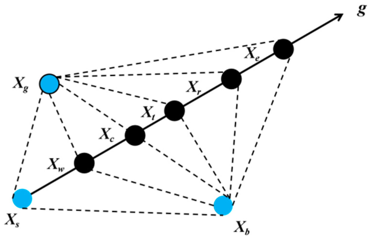
The core idea of the simplex method consists of two stages, and the specific optimization process is shown in
Figure 2. First, randomly generate
N + 1 points to construct a simplex, where
N is the dimension of the desired extreme value. Then, order the function values of these points from smallest to largest, and find the centre of gravity
Xc of the optimal
N points:
The algorithm considers the starting vertex Xs as the worst vertex. The first stage is gradient estimation, in which the direction vectors g from the simplex’s centre to all vertices except Xs are estimated. In the second stage, the worst vertex is iteratively replaced with a new, better vertex. Each vertex corresponds to a solution to the problem. The new vertices are generated through one of four operations: reflection, expansion, outward contraction, and inward contraction.
where
Xr is the reflection point and
α is the reflection coefficient.
where
Xe is the expansion point and
γ is the expansion coefficient.
where
Xt is the external contraction point and
β (
β > 0) is the external contraction coefficient.
where
Xw is the internal shrinkage point and
β (
β < 0) is the internal shrinkage coefficient.
4.2. Differential Evolution Algorithm
The DE algorithm is a kind of metaheuristic evolutionary algorithm. The DE algorithm shows good performance on constrained optimization problems. Therefore, it is often used to solve power system optimization problems [
34].
The DE algorithm first randomly generates N individuals in the search space of the objective function to form the initial population P = {x1, x2, …, xN}. Each individual is a multidimensional decision vector, which can be expressed as xi = (xi1, xi2, …, xiM), where M is the number of decision variables. The DE algorithm realizes population evolution through the following three steps:
The DE algorithm realizes mutation operation through a differential strategy, which is an important symbol different from the genetic algorithm [
35]. For the target vector, that is, each individual
xi = (
xi1,
xi2, …,
xiM) in the population, the difference between any two individuals is added to another individual to produce the mutated offspring
vi:
where
xr1,G,
xr2,G, and
xr3,G are three randomly selected individuals from the G-generation population;
G + 1 in
vi,G+1 represents the
G + 1 generation population; and
i ≠
r1 ≠
r2 ≠
r3.
F is a scale control factor used to determine the size of the difference vector (
xr2,G −
xr3,G).
F is a real number and
F ∈ [0,2].
First, the crossover operator randomly generates a dimensional identification to ensure that at least one dimension of the final test individual is from the mutant individual, so as to avoid the same as the current individual and ensure the diversity of the population. Then, a real number between 0 and 1 is randomly generated for each dimension of the current individual. If the random real number is less than the crossover rate, the dimension of the test individual comes from the variant individual. Otherwise, the dimension of the test individual comes from the current individual.
The mutated offspring
vi and the target vector
xi are crossed over as follows to generate the crossover offspring
ui:
where
randj is a random number with a uniform distribution in [0,1] and
jrand is the dimensional identification, a random integer in [1,
M].
Cr is the crossover probability, which has a value between 0 and 1. In the crossover operation,
j =
jrand guarantees that
ui differs from the target vector
xi in at least one component, thus maintaining the diversity of the population.
The DE algorithm adopts a greedy criterion for selection. It compares the fitness values of
ui and
xi and selects individuals with better fitness as the population for the next generation, which can be expressed as:
where
f denotes the fitness function.
4.3. Improved Hybrid Algorithm
The basic DE algorithm considers only the differential learning between different individuals in the mutation stage, without considering inheritance from and continuous learning of the best-known individual.
Therefore, we propose an adaptive mutation strategy that considers the learning of the best-known individual.
4.3.1. Reconstructing the Uncertain Parts of the Constraints
In practical applications, if
F is set to a constant value that is too large, the convergence rate of the algorithm and the accuracy of the global optimal solution obtained will be reduced. If
F is too small, the diversity of the population will be reduced and premature convergence will occur. To avoid these situations, the value of the parameter
F can be varied with the number of iterations. Specifically, with an increasing number of iterations,
F decreases, thereby preserving excellent population information while avoiding destruction of the optimal solution [
36].
In addition, to increase the inheritance from the best-known individual in the improved method, the mutation operation is expressed as:
where
xbest is the best-known individual, expressed as
xbest = (
xi1best,
xi2best, …,
xiMbest).
F1 represents the differential learning parameter between the current individual and the best individual from the last iteration, which is set to a constant value, usually
F1 ∈ [0,1].
F2 represents the differential learning parameter between the current individual and other individuals in the population, and the value of
F2 is:
where
t is the number of the current iteration and
tmax is the maximum number of iterations. As the number of iterations increases, the search space for the optimal solution gradually increases.
4.3.2. Population Optimization Method
In the hybrid algorithm, the DE algorithm is first used for global optimization and the obtained solutions are sorted in accordance with their performance. Among the first Q individuals, the simplex method is then applied for local optimization. Based on a local learning algorithm and a reverse learning method, a new population of the same size as the remaining number of individuals is generated.
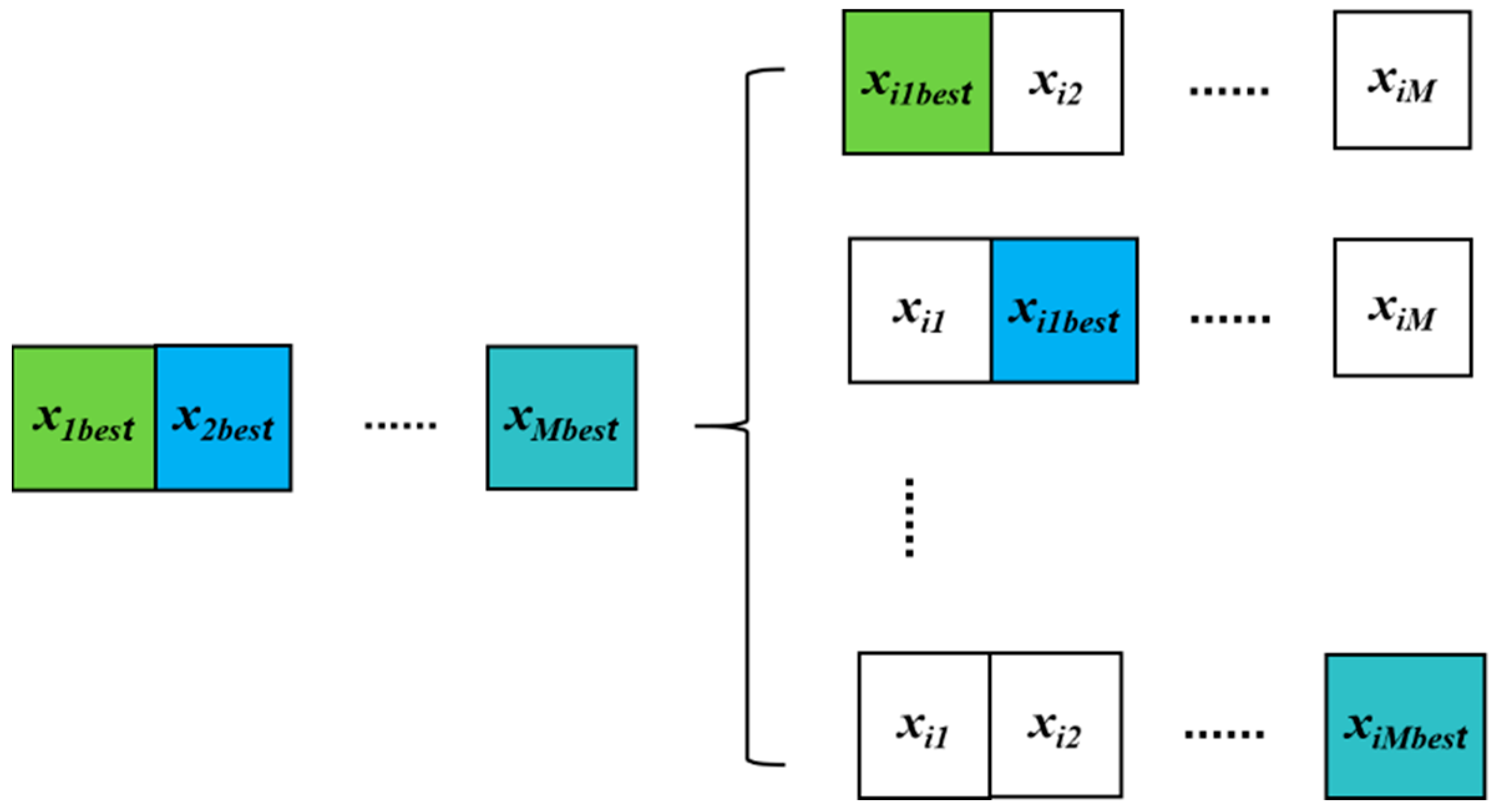
First, a local learning algorithm is used to obtain a new individual based on the value in each dimension of the best-known solution. As shown in
Figure 3, each new individual has the best-known value of one decision variable, and the remaining values are randomly generated, centred on the best-known solution. Thus, we obtain
M new individuals.
Second, the remaining N-Q-M individuals are generated through reverse learning. Reverse learning is designed to improve the learning rate in evolutionary algorithms. Because evolution is a slow process and revolution is a fast process, simulating revolution in evolutionary algorithms may speed up the convergence of the algorithms.
Figure 4 shows the upper and lower limits on
xij and the reverse point
:
For the remaining individuals in the population, the reverse point of each solution is found, and the objective function values of the current solution and the reverse point are compared. If the reverse point has a better target value, then the current solution is replaced with the reverse point; otherwise, the current solution remains the same.
The application of the reverse learning mechanism can make the range of the population search more extensive, and the use of the reverse learning mechanism during population initialization will make the initial population distribution more reasonable.
Evolution is a slow process in a meta-heuristic optimization algorithm. For example, the genetic changes usually take time, but some types of change are very fast. Variation is a rapid change that almost all evolutionary algorithms employ. Reverse learning is designed to improve the learning rate of evolutionary algorithms. Because evolution is a slow process and revolution is a fast process, simulating revolution in evolutionary algorithms may speed up the convergence of the algorithms.
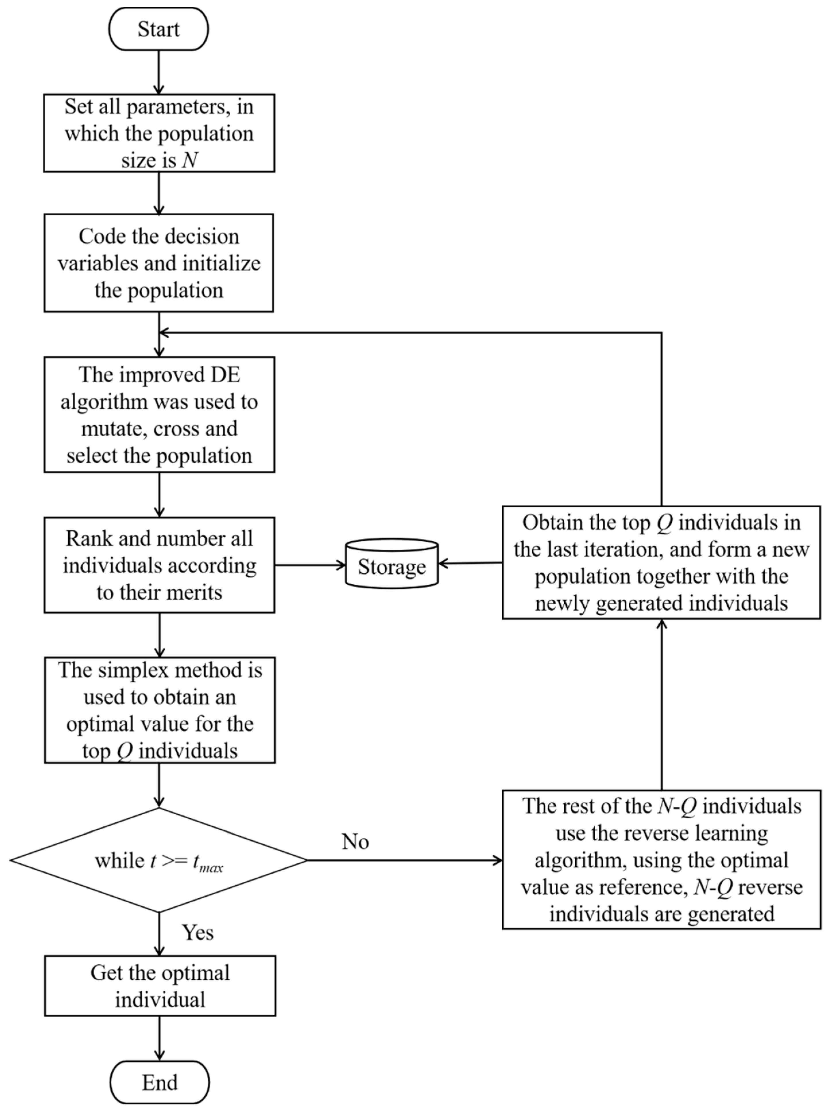
A flow chart of the hybrid algorithm combining the simplex algorithm, the improved DE algorithm, and population optimization is shown in
Figure 5.
As shown in
Figure 5, the initial optimization results are obtained for the target variables after the mutation, crossover and selection operations of the DE algorithm, and then the simplex method is applied to a subset of the targets with good performance to achieve secondary optimization. Thus, on the basis of the DE algorithm, the hybrid algorithm proposed in this paper first performs global optimization for a randomly generated population of the objective function in the feasible domain and then performs local optimization via the simplex method to obtain the optimal solution to the problem.
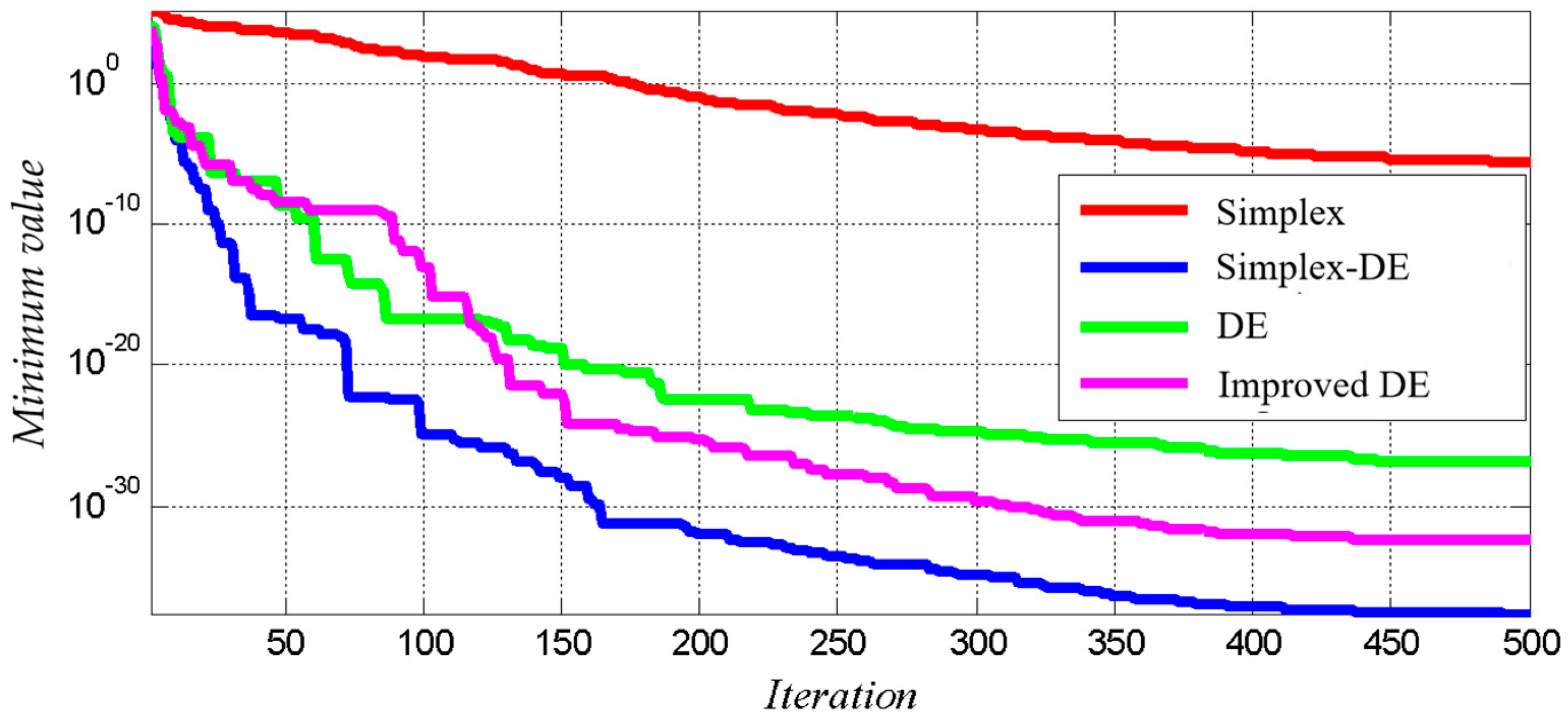
In order to prove the feasibility of the improved algorithm, the test function in Formula (48) was used to test the simplex method, improved differential evolution algorithm, and the hybrid algorithm proposed in this paper. The optimization results are shown in
Figure 6.
where the range of
x is between −100 and 100.
It can be seen from
Figure 6 that the improved hybrid algorithm has better optimization ability for the single objective function.
5. Experimental Analysis
The IEEE 6-Bus system, shown in
Figure 7, was used to verify the performance of the proposed scheduling model and solution algorithm.
The wind farm is set at node 3. Three conventional units G1, G2 and G3 are connected to nodes 1, 2 and 6. L1, L2 and L3 indicate the load. The parameters of the thermal power units are shown in
Table 2.
ai,
bi and
ci are the constant term coefficient, primary term coefficient and secondary term coefficient of unit cost, respectively. The upward and downward reserve cost factors of each conventional unit are set to 10% of its generation cost factor
bi. The power cost factors are adjusted up and down to set the unit production cost under the maximum load state. It is assumed that the climbing capacity of each unit is 40% of its maximum output.
The load demand predictions for nodes 3, 4 and 5 are 100 MW, 150 MW and 150 MW, respectively. Wind farm W is connected to node 3, and the predicted output is 100 MW. The wind curtailment rate limit ηw and the curtailment cost coefficient cw are 0.5 and 100 $/MW, respectively.
First, the number of error samples is taken to be 500 to verify the system scheduling results obtained using the simplex method and the method proposed in this paper under different values of the Wasserstein metric wd. Considering the different units of the input variables in the objective function and constraints, it is necessary to use feature scaling to normalize the objective function and constraints to values between 0 and 1. The violation probability is set to 0.03, the initial scheduling time is set to the next 24 h, and the adjusted scheduling time is set to one hour in advance.
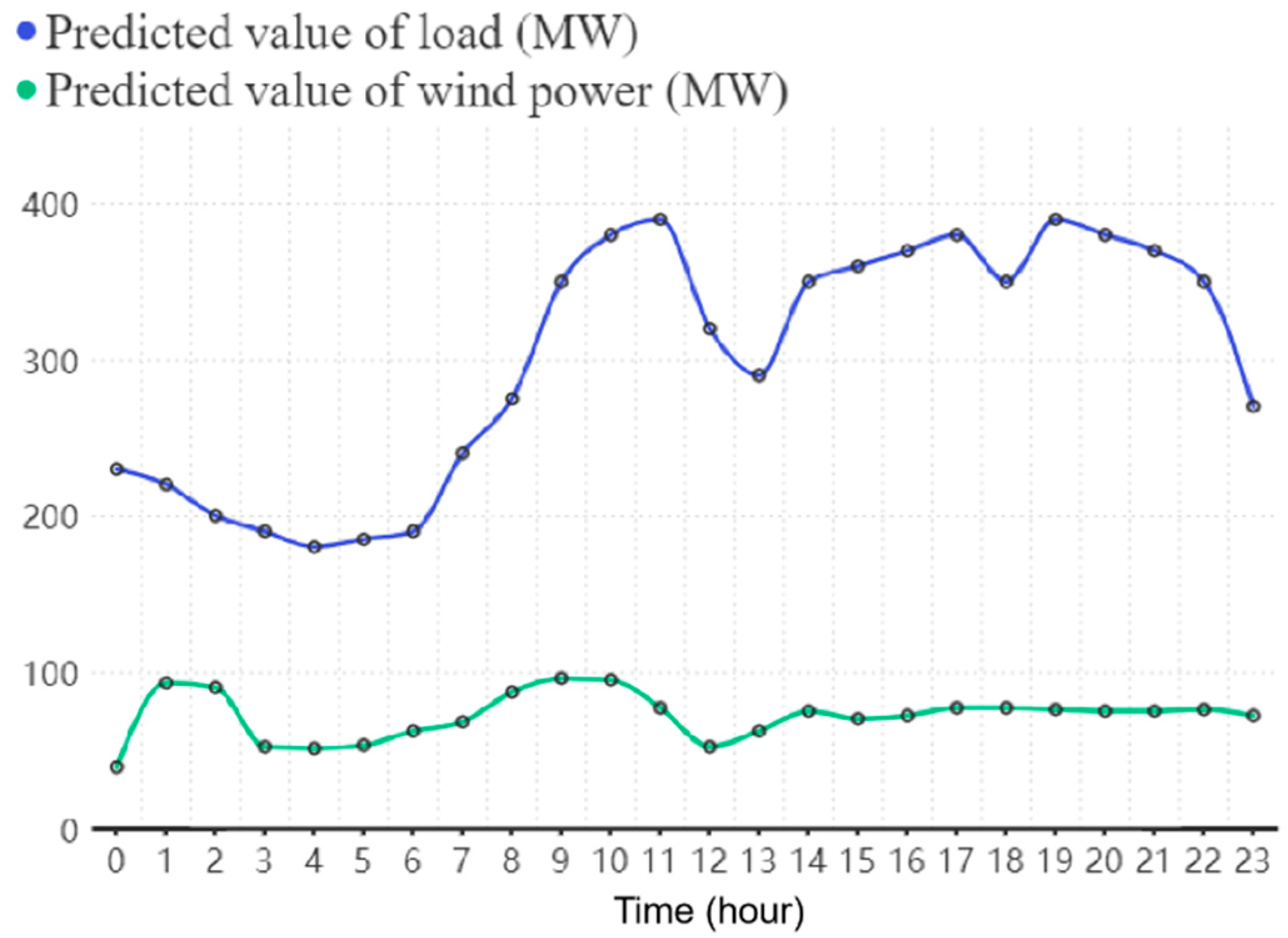
The load data set in this paper comes from a city in northwest China, and the wind power data set comes from a wind farm SCADA in northwest China. For day-ahead scheduling, the load power and wind power in the next 24 h are predicted. The prediction methods are as follows [
37,
38]. The load prediction results and wind power prediction results of the dispatching day are shown in
Figure 8, where the wind power is the predicted result at an interval of 10 min, and hourly wind power output is obtained by calculating the average.
The parameters of the hybrid algorithm include the reflection coefficient,
α = 1; the expansion coefficient,
γ = 2; the internal and external contraction coefficients, both
β = 2; the crossover probability
Cr = 0.1; the number of iterations is 100; and the population size is 500. Meanwhile, as a contrastive experiment, the simplex method is also used to optimize the target directly, with parameter settings consistent with those of the hybrid algorithm.
Table 3 shows the scheduling results when
wd is 0.01.
It can be seen from
Table 3 that when the minimum total objective value of the two-stage scheduling method is taken as the evaluation index, the cost of the proposed optimization algorithm based on the simplex method and the improved DE method is reduced by 456.1 (
$) compared with that of the general mathematical solution method. Thus, it is proven that the proposed method has a better optimization ability.
When the value of the Wasserstein metric
wd is reduced by factors of 100 and 1000 to 0.001 and 0.0001, respectively, the corresponding results of executing the scheduling algorithms are as shown in
Table 4 and
Table 5.
It can be seen from a comparison of
Table 3,
Table 4 and
Table 5 that when Wasserstein metric
wd has a value of 0.001, the total dispatch cost is minimal and the method is optimal. Thus, for the same sample size, a smaller fuzzy set is not better. The smaller the fuzzy set is, the fewer uncertain factors it contains, so the output plan of the thermal power units should be improved from the perspective of power system scheduling. Although the wind abandonment volume is reduced, the total cost is markedly increased. However, it should be noted that if the
wd selection is too large, the problem may become unsolvable.
In addition to the Wasserstein radius metric, the number of random variable samples also affects the results of the algorithm. Accordingly, the results obtained with
wd set to 0.001 and sample sizes
N varying from 10 to 3000 are shown in
Table 6.
As shown in
Table 6, the optimization results vary greatly with the number of samples. As the number of samples increases, the total cost decreases for both methods. Specifically, when the sample size is increased from 10 to 100, the target costs of the simplex method and hybrid algorithm are reduced by 879.8 and 839.3, respectively. This is because an increase in the number of samples reduces the allowable deviation limit of the probability distribution in the fuzzy set, thus reducing the degree of conservatism in solving the problem. Therefore, for the same value of the Wasserstein metric, the optimization results are affected by the number of samples.
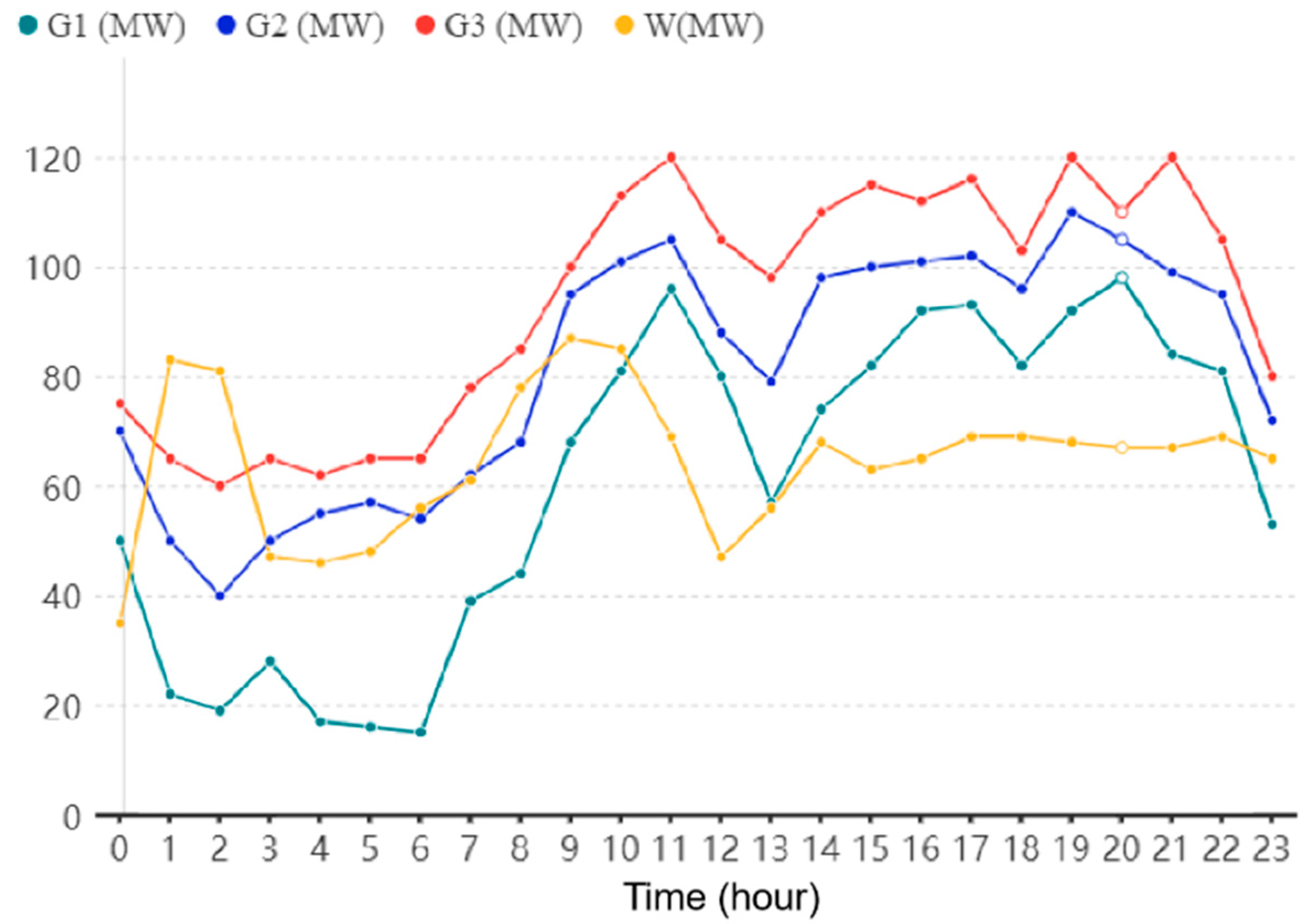
Under the optimal scheduling, output curves of each thermal power unit and wind power farm are shown in
Figure 9. Compared with the G1 thermal power unit, G2 and G3 have lower dispatching costs so they have a larger dispatching output. The wind farm output on this dispatching day is relatively stable.
