Article

Joint Modeling of Wind Speed and Power via a Nonparametric Approach

by
Saulo Custodio de Aquino Ferreira
,
Paula Medina Maçaira
and
Fernando Luiz Cyrino Oliveira
*
Industrial Engineering Department, Pontifical Catholic University of Rio de Janeiro (PUC-Rio), Rio de Janeiro 22451-040, Brazil
*
Author to whom correspondence should be addressed.
Energies 2024, 17(14), 3573; https://doi.org/10.3390/en17143573
Submission received: 19 June 2024 / Revised: 11 July 2024 / Accepted: 16 July 2024 / Published: 20 July 2024
(This article belongs to the Special Issue Recent Development and Future Perspective of Wind Power Generation)

Abstract

:
Power output from wind turbines is influenced by wind speed, but the traditional theoretical power curve approach introduces uncertainty into wind energy forecasting models. This is because it assumes a consistent power output for a given wind speed. To address this issue, a new nonparametric method has been proposed. It uses K-means clustering to estimate wind speed intervals, applies kernel density estimation (KDE) to establish the probability density function (PDF) for each interval and employs Monte Carlo simulation to predict power output based on the PDF. The method was tested using data from the MERRA-2 database, covering five wind farms in Brazil. The results showed that the new method outperformed the conventional estimation technique, improving estimates by an average of 47 to 49%. This study contributes by (i) proposing a new nonparametric method for modeling the relationship between wind speed and power; (ii) emphasizing the superiority of probabilistic modeling in capturing the natural variability in wind generation; (iii) demonstrating the benefits of temporally segregating data; (iv) highlighting how different wind farms within the same region can have distinct generation profiles due to environmental and technical factors; and (v) underscoring the significance and reliability of the data provided by the MERRA-2 database.

1. Introduction

The growing demand for energy from renewable sources has led to the construction of many wind farms in Brazil and other countries. However, two main factors can hamper the development of the wind power industry: the probabilistic nature of wind speed and the uncertainty involving its production [1,2]. These factors require more robust and reliable models that better replicate the behavior of local wind generation to support the planning, monitoring and operational management of the power grid and increase the reliability of the electrical network [3,4,5,6].
For the correct dimensioning of power generation, it is necessary to understand the functioning of wind turbine generators [1]. It is well established that the power from a wind turbine varies in function with the wind speed, air density and turbine blade parameters (size, design, tip speed and pitch angle ratio) [7]. The manufacturers usually supply a power curve for their models, which is typically generic and related only to the wind speed for the power generated [8]. Nevertheless, this information serves as a parameter for initial monitoring of the performance of a wind farm’s turbines [9].
For managers of wind farms and power systems, it is not advisable to apply the manufacturer’s power curve directly since the real working conditions of a turbine can be very different. The power curve made available by the manufacturer is projected for the functioning of a single wind turbine operating under ideal conditions. It does not consider the various types of interference they generate with each other within a wind farm. Hence, a need exists to develop models to estimate wind power in specific generation locations [9].
Researchers have described various deterministic or probabilistic strategies to create reliable estimation models. These power curve models are also subdivided into parametric and nonparametric techniques [7,10,11]. The parametric methods are based on mathematical formulations, such as the linearized segmented model; polynomial power curves [12,13]; exponential [14], cubic [7] and maximum principle methods; the least squares method [10]; cubic spline interpolation; dynamic power curves; and models based on probabilistic distributions [6,10,15], among others. In general, they are methods that are easy to apply and calculate the parameters, need little historical data, and have precise adjustments. Their drawbacks are poor accuracy, the need for comprehensive data from the manufacturer and the local conditions, and failure to consider the variability of these data [11].
The nonparametric models include copulas [16,17], kernel density estimation, artificial neural networks [18], fuzzy logic systems, support vector machines, response surface methodology and data mining algorithms (such as random forest and clustering) [18], among many others [9,19,20,21,22]. These do not impose any model specified in advance, are more precise, contemplate the variance of the data and estimate the power curve as closely as possible with the available data subject to smoothing of the fit. However, these methods require long historical data series and are complex to implement [11,23].
In [18], the authors used machine learning, artificial neural networks (ANNs), decision trees (DTs) and random forests (RFs) to infer the best alternative to represent the outputs of a wind turbine. The same evaluation is described in [23] via three dynamic Bayesian models considering wind speed and power. In turn, refs. [16,17] propose the use of copula functions to model this relationship through the measured data, while [16] also uses a probabilistic method to exclude outliers. The article by [24] evaluates the performance of multivariate models based on the Gaussian mixture copula model (GMCM), artificial neural networks and Bayesian artificial neural networks (BANNs) to characterize the power curve and estimated power.
Many other studies have also used wind speed distribution as a basis to model the relationship between wind speed and power output. Most of these have recommended using a two-parameter Weibull distribution [25]. More recent studies have suggested modifications of the Weibull distribution [26] and the use of a four-parameter Kappa probability distribution or five-parameter Wakeby probability distribution to obtain better results [27].
In [7], the authors describe the fitting of polynomial, exponential and cubic equations to represent the power curves of turbines. The authors found the polynomial and cubic approaches to be most precise. Still, the polynomial approach required complex equations, making it hard to find a general expression, leading to the recommendation of the cubic, which only depends on the parameters provided by the manufacturer. Ref. [11] warns that these mathematical models should only be used for initial evaluation of the power output, because they do not precisely consider the inflection point of the power curve and can result in large forecasting errors. They serve to evaluate new undertakings, dimensioning and the optimization of costs. Ref. [28] suggests using sigmoid, logistic and Hill functions, while [10] proposes the spline regression method to obtain better performance and overcome the problems of determining the curve’s inflection point. However, although these mathematical expressions are widely used, there is little evidence that these curves fit the data pertaining to real wind power turbines [12,13,14].
For this reason, this study aims to describe a model that more accurately represents this relationship between wind speed and power, requiring only historical data for both variables. Although the method uses only these two data points, it can indirectly incorporate the complexity inherent in the variability of the different sources of meteorological data and those specific to the turbine designer, which can also influence the prospection of the resulting wind energy.
In this context, a method is presented to segment the wind speed ranges through clustering data by K-means, mapping possible wind power outputs associated with each range and constructing the probability density function of the power data using the kernel density estimation method. Finally, the Monte Carlo simulation is applied to make the model flexible regarding wind power generation.
To improve the modeling of the relationship between wind speed and wind energy generation, this paper combines these methods to create a more reliable and effective methodology. This will help us make more accurate projections that align with real-life conditions in wind turbines. Once implemented, this model will enable us to use wind speed projections to estimate wind power effectively.
This article is divided into five sections, including this introduction. The second section presents the method used to model the relationship between wind speed and power; the third section presents the data used in the tests; the fourth section describes and discusses the results; and the fifth section presents the conclusions and some recommendations for future research.

2. Proposed Methods

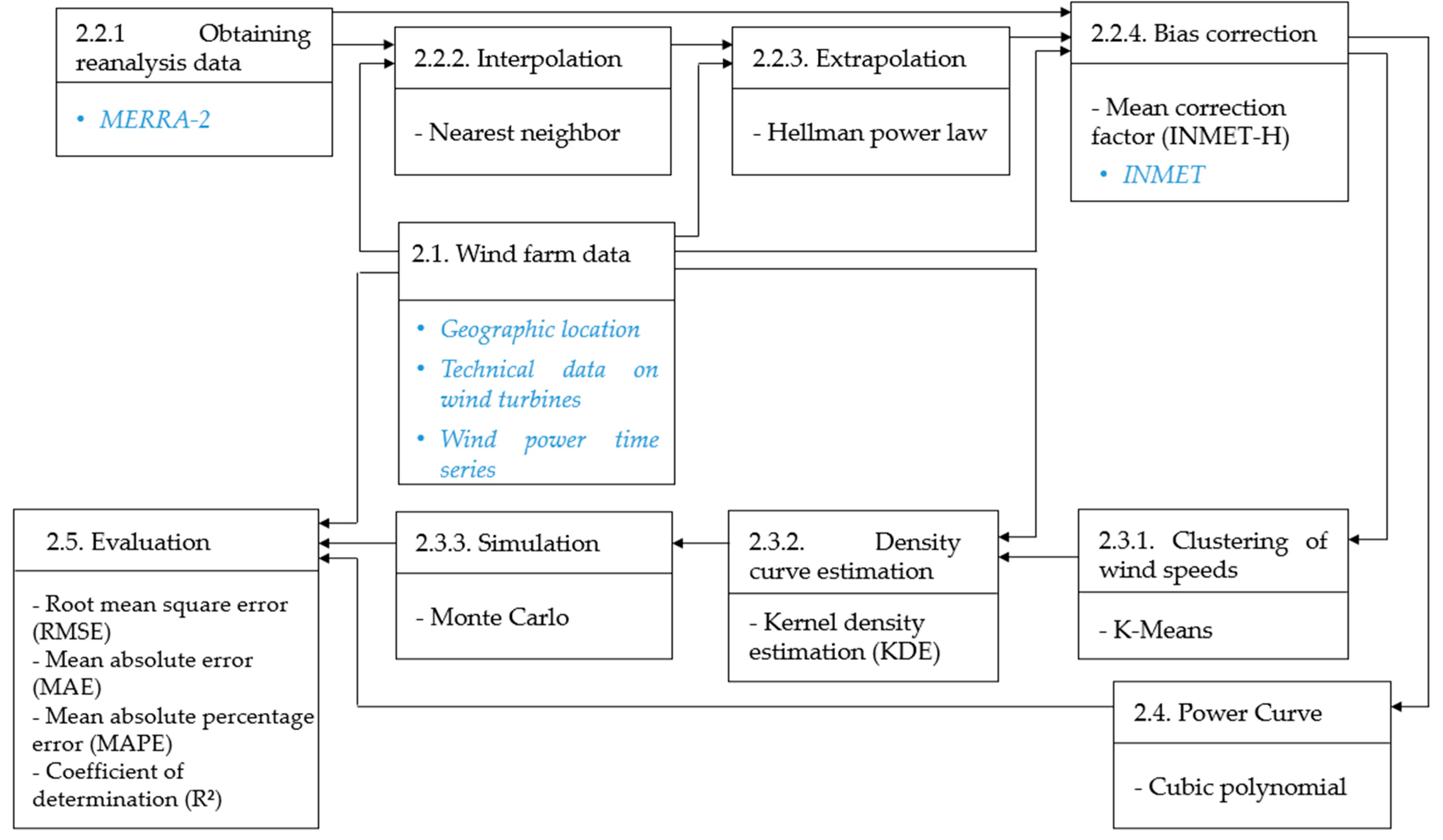
The purpose of this article is to describe a method that can model the nonlinear relationship between the speed of the wind that passes through wind turbines and the power generated by them, thus enabling the exploration of the peculiarities of the source and place and the depiction of the probability distribution of generation for a given wind speed value. The steps used in this study to attain this goal are presented in Figure 1.
Section 2.1 presents the locations used to test the proposed method. Section 2.2 summarizes the steps employed in the predecessor contribution [29], which details steps 2.2.1 to 2.2.4. It discusses how to obtain and treat the wind speed reanalysis data from MERRA-2 for points in Brazilian territory to have data representing local reality and overcome the shortage of measured data points. We describe the main contributions of this article in Section 2.3.1, Section 2.3.2 and Section 2.3.3 regarding the wind power modeling and forecasting method. Section 2.4 presents a simple and widely adopted method to compare our proposal here against other methods used to relate wind speed and wind power generation. Finally, Section 2.5 offers the metrics adopted to evaluate the method.

2.1. Wind Farm Data

To test the method presented in this article, information from five wind farms located in the same state in Brazil’s Northeast Region is used; three farms are along the coast and the other two are in the interior of the state. The information the wind farm managers provided included the geographic locations, installed capacities and generation time series, which cannot be disclosed due to a secrecy agreement.
The other information necessary to apply the method, such as the technical characteristics of the turbines used by the wind farms, was obtained from the Electric Sector Georeferenced Information System of Brazil’s National Electric Energy Agency (SIGEL/ANEEL) [30] and The Wind Power database [31].
These wind farms were chosen due to the convenience of measuring data availability and their location in the Northeast Region, where there is significant wind potential, the number of wind plants has grown and methodologies are needed to help their work [23,29,32,33].

2.2. Wind Speed Data

The wind farms chosen for testing do not have any wind speed history, only historical generation data. However, the power generated by these turbines is directly related to the wind speed at the height of the corresponding rotor, and modeling this relationship is the purpose of this article.
To overcome this limitation, MERRA-2 reanalysis data were used [34]. They provide a free historical series on climate variables and atmospheric data since 1980, available at grid points covering the Earth’s entire land surface. The MERRA-2 databases used most often are “MERRA-2 tavg1_2d_slv_Nx” and “MERRA-2 inst1_2d_asm_Nx” to obtain historical wind speed data. The main difference is that the wind speed data are hourly averages in the former, and in the latter, the data are collected instantaneously. The first database was adopted for this study because it presented the best results in preliminary tests and the wind power data were also hourly averages [34].
Interpolation, extrapolation and bias correction were used to adjust the wind speed time series of MERRA-2 to the natural conditions of the turbines in question [29]. The interpolation adopted was based on the nearest neighbor technique, which consists of obtaining the data from the point on the MERRA-2 grid closest to the geographic location of the wind farm to represent the speeds that occurred at that point. In turn, the power law is used as the extrapolation technique to adjust the historical wind speed data of MERRA-2 to the values that occurred at the hub height [32]. Finally, bias correction involves applying an average hourly correction factor using data from the nearest National Meteorology Institute (INMET) station. This technique consists of calculating the hourly wind speed averages of the MERRA-2 and INMET datasets at the same height (in this case, 10 m) and calculating the ratio between them each hour to generate an hourly correction factor to be applied to the extrapolated wind speed time series to adjust it to the real winds measured in Brazilian territory and contemplate the local particularities [13,20]. This method is suggested by [29] to obtain data from MERRA-2 for Brazil.

2.3. Modeling the Speed Versus Power Relationship

A particular wind speed value can generate different power values from the same turbine at distinct moments. A combination of factors, such as variations in wind direction, relative air humidity, atmospheric pressure and other climatic and atmospheric variables, can explain this. However, mapping all these wind generation variations in the function of such variables would make the model highly complex and still would not assure the identification of all the factors that can impact the generation [7].
Thus, this proposed methodology seeks to simplify the modeling of wind generation to enable its projection using a single variable, the wind speed, striving to create a model that explains all the randomness arising from the various data sources solely according to wind speed. To materialize the idea, the wind speeds that can occur in a wind farm are segmented, and each range’s generation possibilities are dimensioned based on the speeds that are believed to occur. The techniques used to materialize this method are presented in Section 2.3.1 Section 2.3.2 and Section 2.3.3.

2.3.1. Clustering of Wind Speeds

The K-means algorithm assigns each input data point to a group, also known as a cluster, and seeks to minimize the sum of squares within each group [21,35]. This article uses this technique to identify the wind speed ranges. It groups the wind speed data into k clusters (speed range groups), where each data point is assigned to a cluster with more similar data. This approach is an alternative to using multivariate probability density functions and reducing the problem’s dimensionality using coupling speeds that can be considered similar behavior.
The technique’s algorithm starts by randomly defining k centroids (centers of clusters). Then, the distance is calculated between each data point and the initial k centroids, and the value is attributed to the nearest cluster. Next, new centroids are defined, each being the average of all the data composing the respective cluster. This process is repeated until the centroids remain fixed after multiple iterations [22].
The K-means method has a premise consisting of the number of clusters, k , to be adopted. Hence, to find the most suitable number of clusters, the elbow method is used, which is applied by gradually increasing the number of clusters, and with each addition verifying whether, on average, the standard deviation of the clusters is reduced, such that the accuracy of the centroid reflecting the historic data is increased. Thus, the number of clusters is defined when the variations of the standard deviation become negligible when including another cluster [36].

2.3.2. Density Curve Estimation

Since power generation is a continuous variable, and it was desired that the frequency of its values for each cluster of velocities was understood, the probability density function (PDF) was estimated for the generation of each cluster. This association is possible because each wind speed value is associated in time with a historic occurrence of wind farm generation.
The technique used to estimate the probability density functions is kernel density estimation (KDE), a nonparametric estimation approach. Its main advantage is that it is not necessary to assume the distribution of the sample data in advance, thus avoiding the introduction of subjective previous information. This allows for a generalization of the proposal independent of the data used [37,38].
Since the KDE involves fitting the density function concerning the data, this process is more precise and robust compared to parametric approaches [37]. If x denotes the sample dataset, f x can be expressed as in Equation (1):
f x = F x = F x + h F x h 2 h ,
where h is a non-negative constant, called the bandwidth, and F x represents the empirical distribution of the power data that compose the sample.
To assure a better fit of the probability distribution, the sample size is allowed to tend to infinity ( n ) and the bandwidth to zero ( h 0 ) [37,38]. Hence, the expression for the estimator of f x can be defined as in Equation (2):
f ^ x = 1 n h i = 1 n K x x i h ,
where K ( . ) is the kernel function. Based on Equation (2), note that the determination of the estimates, f ^ ( x ) , mainly depends on h and K ( . ) [35].

2.3.3. Simulation

Monte Carlo simulation is a statistical method that uses a large number of random samples to obtain numerical results that would previously be deterministic [39]. It was used to guarantee the variability in wind energy generation as a function of wind speed.
According to the previous steps, each speed range from a cluster has an associated probability density function, for which the cumulative density function is calculated. This randomly generates a value from a uniform [0, 1] distribution, which is used in the cumulative function to find the power value that produces the corresponding cumulative probability [6,10,39,40].
In order to calculate the power values, one needs to determine which cluster the next wind speed value belongs to and find the corresponding cumulative function. Then, a new random probability value is generated for the cumulative function. This process is repeated until the sequence of wind power generation estimates is completed [38].

2.4. Power Curve

The conventional deterministic approach to obtain the available power of the wind passing through the rotor-swept area is expressed in Equation (3) [7,41]:
P t v = 1 2 A ρ v 3
where P t v is the theoretical power generated in watts when the wind speed v , in m/s, passes through a turbine with rotor area A , in m2, and ρ is the air density.
However, the real power generated, P r v , is lower than P t v due to mechanical and electrical losses and the aerodynamic factors of the blades. The ratio between the powers generates the power coefficient, C p , which is typically available from the turbine manufacturer. The theoretical maximum value of the power coefficient is 0.593, the Betz limit, but in practice this value is not attained in the turbines, with the maximum value being 0.5 [6,7].
Equation (4) represents this mathematically:
P v = 0 , v < V C i P * ( v ) , V C i v < V r P r , V r v V c o 0 , v > V c o
where P v is the electric power generated, V C i is the initial cutoff wind speed, V r is the nominal wind speed, V c o is the final cutoff wind speed, P r is the nominal power and P * ( v ) is the power related nonlinearly to wind speed.
The format of the nonlinear part of Equation (4) is related to the strategy of controlling the maximum power extraction from the wind, which is normally moderated by a cubic power curve, as expressed in Equation (5):
P * v = 1 2 π   r 2 C p   ρ v 3
where r is the rotor radius [7].
The regions identified in Equation (4) are not clearly demarcated in the operation of the wind turbines. The corresponding wind speeds that delimit the regions are found from averages of repeated measurements. This is another limitation of this approach [7,23].

2.5. Evaluation

The evaluation metrics adopted in this study were root mean square error (RMSE), mean absolute error (MAE), mean absolute percentage error (MAPE) and coefficient of determination (R2). These are the most commonly used and recommended in the literature [3,7,18,27,36,37,39,42,43,44]. They measure to what extent the real (observed) power values differ from those predicted by the techniques used, reproducing the degree of dispersion between the two metrics. The RMSE and MAE are expressed per unit (p.u.), while the MAPE and R2 are expressed in percentages.
In the first three metrics, lower values are associated with better performance, while for R2, higher values mean a better result.

3. Data

This section presents the data used in this study and their descriptive analyses.

3.1. Wind Power Data

The historical time series from the wind farms are the hours of active power and did not need treatment. There were no missing data, power levels higher than installed capacity, or negative power values. There were differences in the historical dimensions of the wind farms due to their different startup dates. The farms located along the coast are the oldest and have been in operation for 9 years and 2 months (1 January 2013 to 28 February 2022), while those located inland have only been operating for 4 years and 4 months (1 November 2017 to 28 December 2022). The other data necessary to apply the method, such as the technical characteristics of the turbines, were obtained from the SIGEL/ANEEL platform [30] and are presented in Table 1.
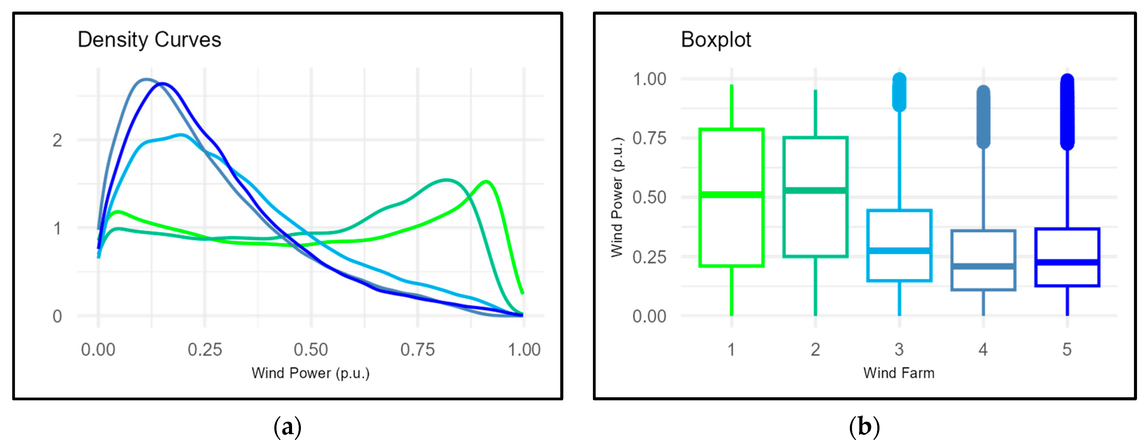
Figure 2 and Figure 3 depict the characteristics of the historical data on the active power of the wind farms. Power data are used p.u. (per unit), which consists of dividing the registered powers by the maximum power. This is carried out to make a fairer comparison between wind farms and the generation of different orders of magnitude. From Figure 2a, it can be noted that the probability density functions of each region are similar. The density curves of the wind farms on the coast are unimodal, with a top value near 10% of the installed capacity. In contrast, the density curves of the interior wind farms are bimodal, with peaks at the extremes. The power data from interior wind farms are more variable than those on the coast, and higher power values are also rarer due to the presence of outliers in their boxplots, as illustrated in Figure 2b.
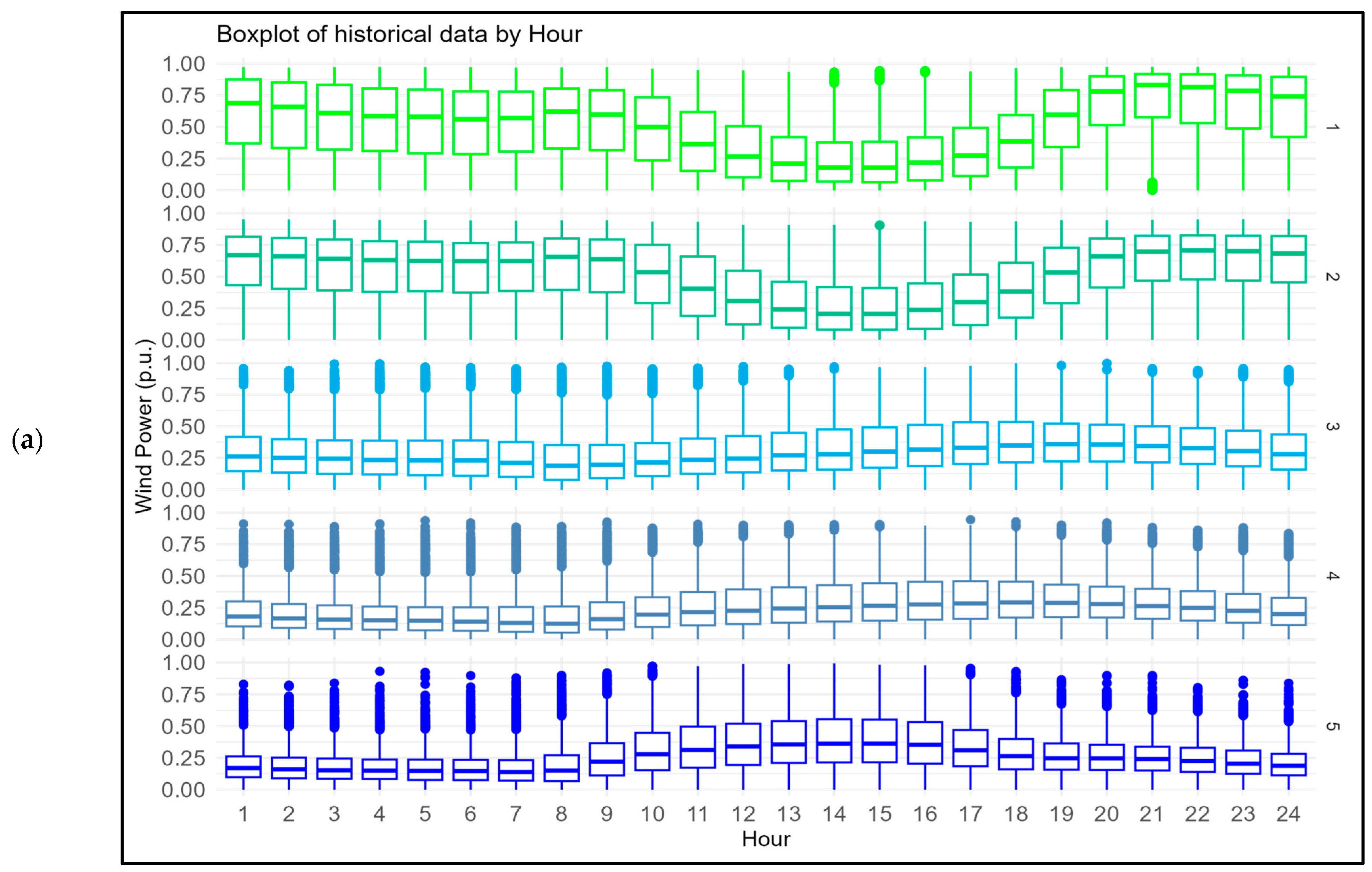
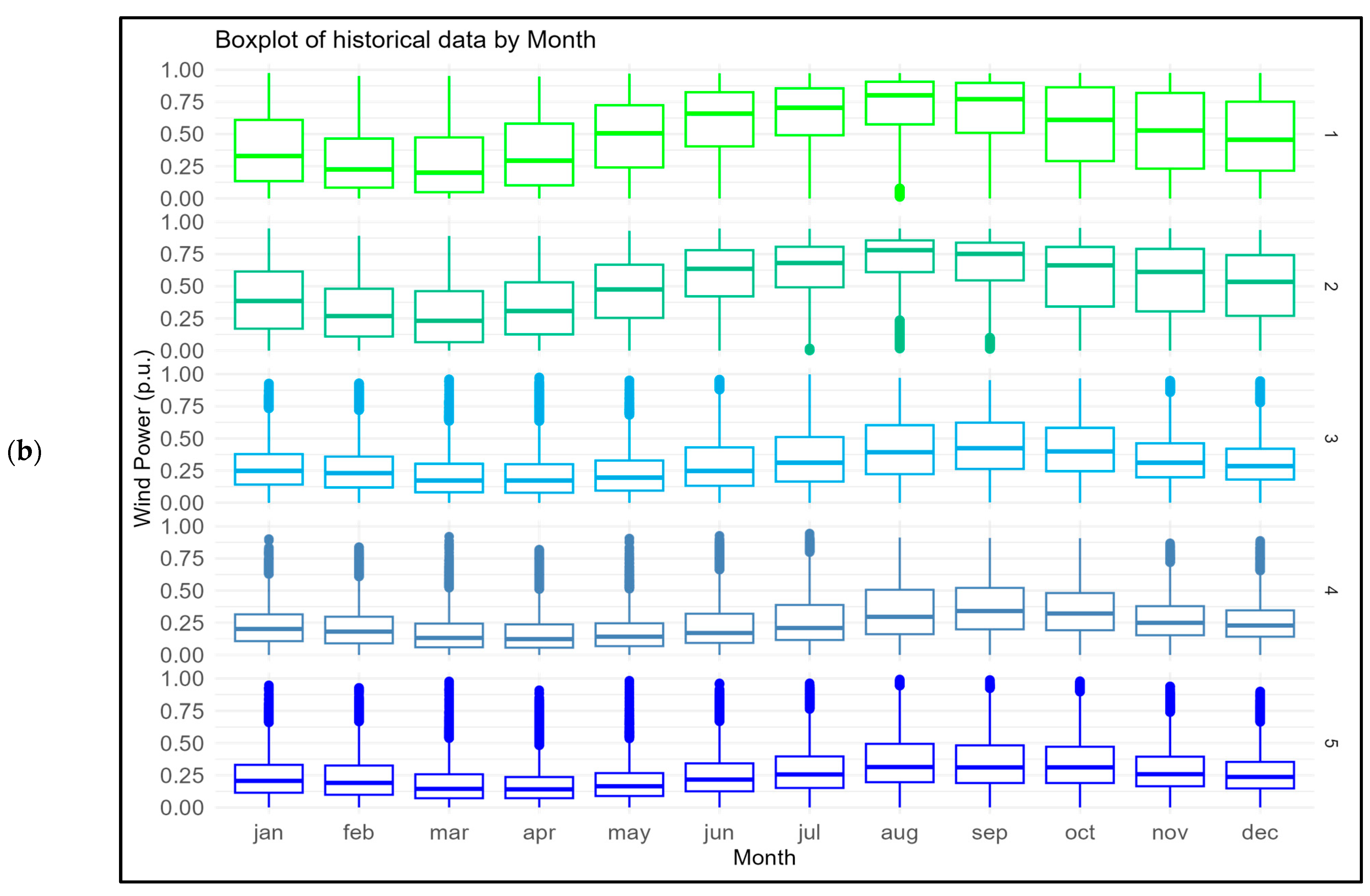
Figure 3 presents boxplots that indicate the generation variability during the different hours and months of operation. The wind farms in the interior have the lowest generation during the afternoon, while those located along the coast have highest generation during that period. Nevertheless, from a monthly standpoint, all the wind farms had higher generation during the year’s second half, with peaks in August and September.

3.2. Wind Turbines

Although the theoretical power curve has apparently well-defined regions, the limiting speeds of those regions vary compared with the manufacturer’s specifications. The turbine models used by the wind farms examined in this study are identified in Table 2. This information was obtained from a previous study [7] and The Wind Power database [31].

4. Results and Discussion

This section will present the results of the wind power estimates achieved by the traditional approach and the different application strategies of the proposed method. The work presented here was developed using R software, version 4.3.0 [45].
Table 3 presents some of the data used and calculated in adjusting the wind speed time series from MERRA-2 to each wind farm’s conditions. Gruber et al. [32] recommend applying the bias correction step to MERRA-2 data only when the INMET station is 40 km from the wind farm. Otherwise, bias correction is not advisable due to the considerable distance between the station and wind farm, such that the INMET data may not adequately represent the real local conditions of the wind farm.
In this study, certain wind farms were situated over 40 km away from an INMET station. To assess the influence of utilizing these data in bias correction, tests were conducted on the wind speed time series both with and without bias correction.
Other information used to generate the results of this work, such as the geographic coordinates of the points on the MERRA-2 network closest to the wind farms and INMET stations, is not shown here due to the confidentiality agreement signed with the wind farm operators.
With the wind speed data, the wind power estimations were made using different techniques and approaches. The theoretical power curve method used the information from the manufacturer presented in Table 2 to delineate the regions of zero, constant and variable generation in terms of the wind speed, as depicted in Equation (4).
The modeling of the nonlinear region was performed with the cubic power curve presented in Equation (5), with the parameter ρ set to 1.16 kg/m3, as recommended by [46]. The C p values were adjusted empirically to enable the maximum power to be found at the nominal wind speed; the other parameters of the curve were assumed to be known and accurate to adjust [46]. Comparing the power outputs generated by the curves based on the wind speed time series with the historical power time series through the evaluation metrics, the results will be listed.
The results achieved with the traditional cubic power curve approach were used to develop the steps of the proposed method, which was tested in four approaches: single-period, monthly, hourly, and monthly–hourly.
In the first step of the proposed method, K-means clustering was performed only once with all data in the single-period approach. In the monthly approach, the clustering was carried out 12 times, each with the wind speed data for the respective month, while this was 24 times in the hourly approach and 288 times in the monthly–hourly case. In all cases, defining the number of clusters with the elbow method was first necessary. In the single-period approach, the number of clusters varied from 20 to 22, in the monthly case it ranged from 17 to 22, in the hourly case it ranged from 12 to 20, and in the monthly–hourly case it ranged from 3 to 14. Table 4 details the number of clusters used in each test. Irrespective of the wind farm and the steps adopted to construct the wind speed time series, the number of clusters defined with the elbow method for applying clustering was practically the same, only diminishing when the data segregation was increased to apply the new proposed method.
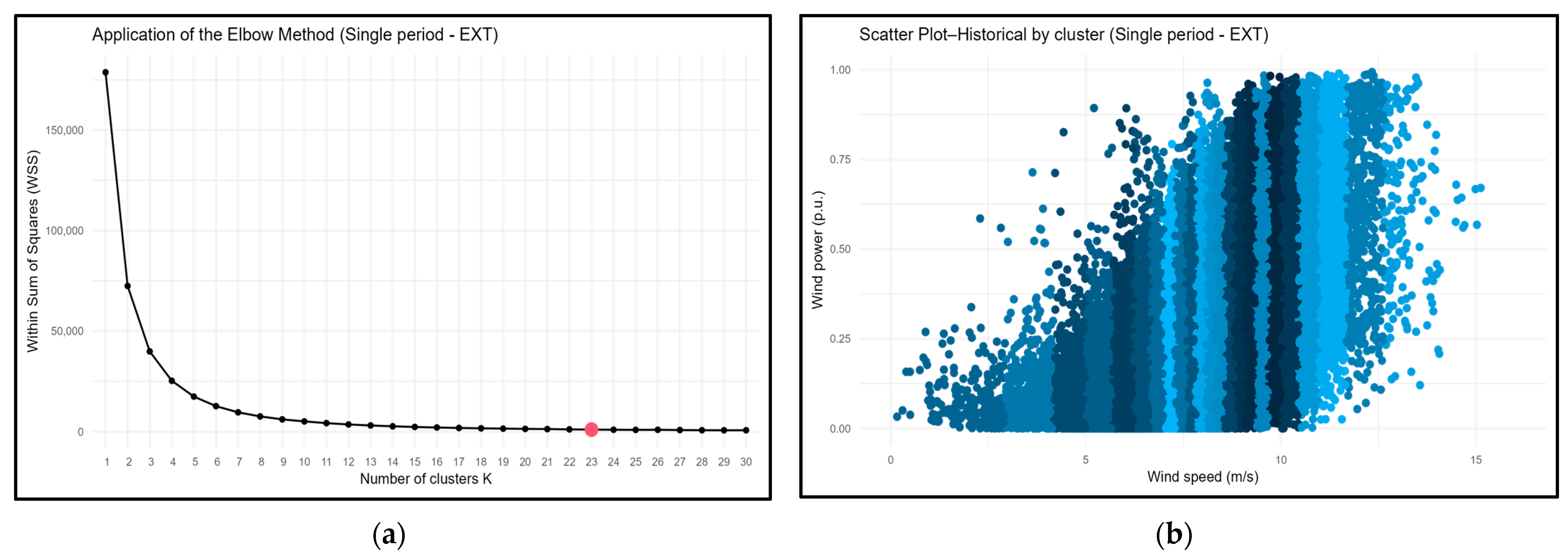
Figure 4 presents the result of applying the elbow method to Wind Farm 5 using a single period with extrapolated speed data (single-EXT) and a dispersion graph of the speed and power data. In the second graph, the different blue shades indicate the different wind speed clusters, permitting visualization of the variability in the power levels generated in each speed range. Corresponding graphs for the other farms and approaches are contained in the Supplementary Materials.
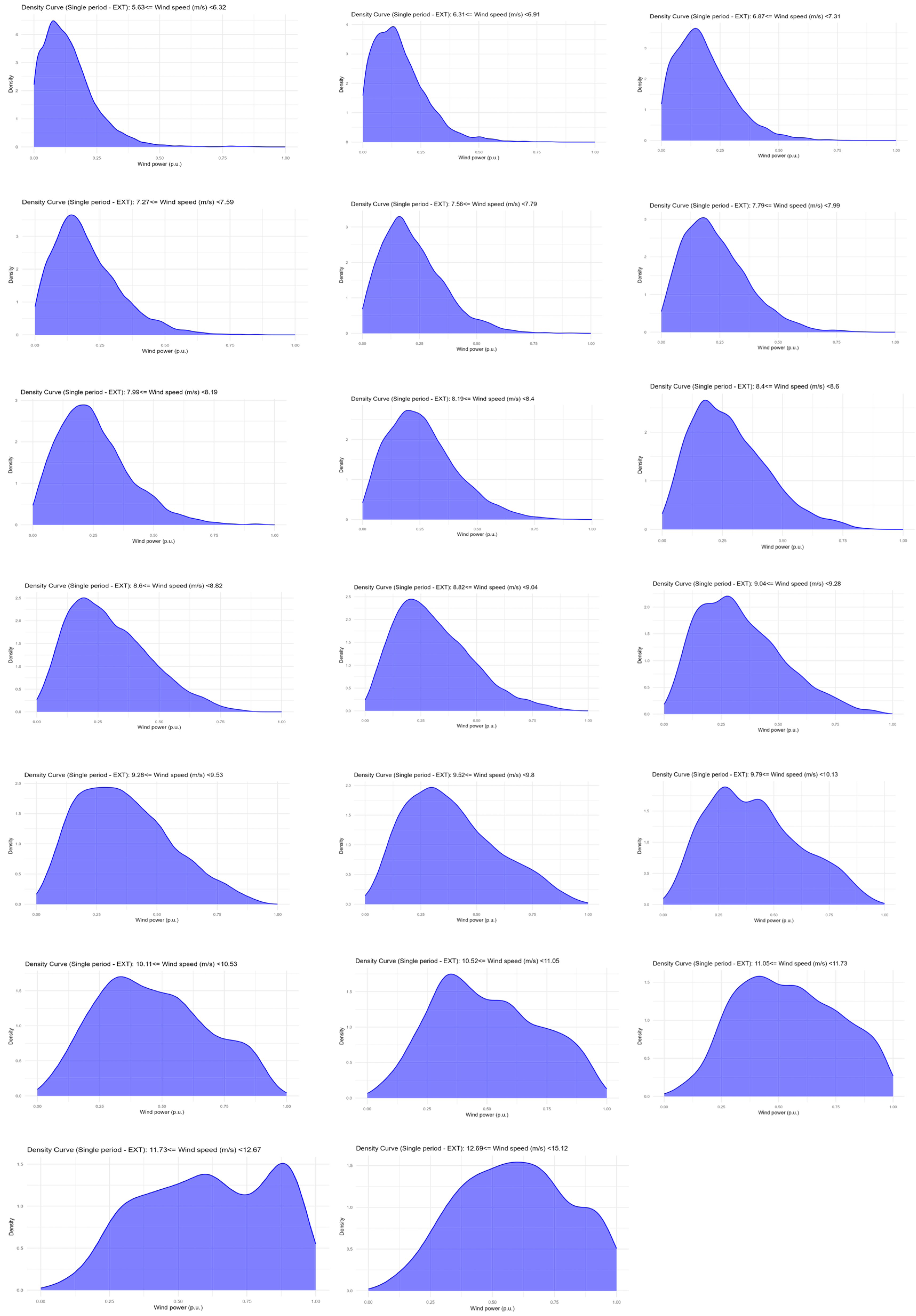
Then, KDE was applied to estimate the probability density function of the power values for each cluster resulting from the previous step. Figure 5 contains the PDF resulting from this step for each wind speed interval on Wind Farm 5 by the single-EXT approach. Note that as the wind speed values of the intervals increase, the peak of the density curve shifts toward the end of the interval. This behavior was seen for all the wind farms and approaches and was expected since faster wind speeds tend to generate more energy. Figures with the probability distributions of all the speed ranges for all the wind farms and approaches are shown in the Supplementary Materials.
It is important to mention that the KDE technique adopted in this work, based on [37,38], generates probability distributions that can infer negative power values. Other methods were tested, such as KDE Beta, but the results were worse, as observed by visualizing the graphs and the evaluation metrics. This highlights the great advantage of kernel density estimation, which adjusts according to the data and allows the proposal to be generalized regardless of the data used.
To emulate the variability in the behavior of a turbine in operation, Monte Carlo simulation was performed, which requires the wind speed time series and the density functions of the clusters. In applying the simulation for a single period, only the PDF utilized varied based on the generating wind speed cluster. At the same time, in the approaches with temporal segmentation, the choice of the PDF changed due to the wind speed and instant of time for estimating the wind power.
To measure the quality of the results, the metrics RMSE, MAE, MAPE and R2 were used, compared to the active, historical and estimated power time series. To construct the estimates using the method proposed here, 100 power time series simulations were generated, and each time point’s average power was calculated. The number of scenarios adopted was found experimentally by ceasing to increase the number of scenarios when no further gains were obtained based on the evaluation metrics (only increases in computational cost). Table 5 depicts the results obtained by the different estimation strategies, with the best result of each test highlighted in boldface. Note that irrespective of the evaluation metric, wind farm analysis or steps adopted to construct the wind speed time series employed in the test, the new proposed method always performed better than the cubic power curve, and the monthly–hourly strategy was the best in all cases.
Regarding the new proposed method, as the segmentation of the data for applying the three techniques increased, the simulations based on the metrics indicated in Table 5 improved, with only one exception. In the test of Wind Farm 3 using speed EXT data, the monthly approach performed better than the hourly approach, as identified by the four evaluation metrics.
Table 6 and Table 7 detail the results of Table 5, where it is possible to see the behavior of the RMSE metric by month and hour in each test, respectively, and verify whether a trend exists other than that observed in Table 5. Again, the best performance was achieved by the monthly–hourly approach in all the wind farms in all months and hours. Nevertheless, in a few isolated months and hours, the theoretical power curve method performed better than the proposed technique, with the single-period and monthly approaches being better than the hourly approach. All these analyses were carried out using the metrics MAE, MAPE and R2; the respective tables are in the Supplementary Materials. The conclusions were the same as those with the RMSE.
The type of treatment applied to wind speed did not influence the performance of the modeling strategies presented here for the evaluation metrics. Mainly, it did not impair the identification of the best approach to estimate the wind power. Thus, as pointed out in a previous study [29], the wind speed time series data that only underwent interpolation and extrapolation (EXT) also achieved a good representation of the series measured on the farms; in some cases, this was better than the series that underwent the third step, bias correction (INMET-H). This might have happened because the quality of the correction is directly related to the quality and quantity of measurements supplied by the INMET station and its distance from the wind farm. It is not always possible to satisfy these factors. For example, the EXT series produced better performance at Wind Farms 1 and 2, where the maximum distance requirement between the farm and INMET station was not satisfied. At the other wind farms, the best performance between the two treatment options in the monthly case was alternated.
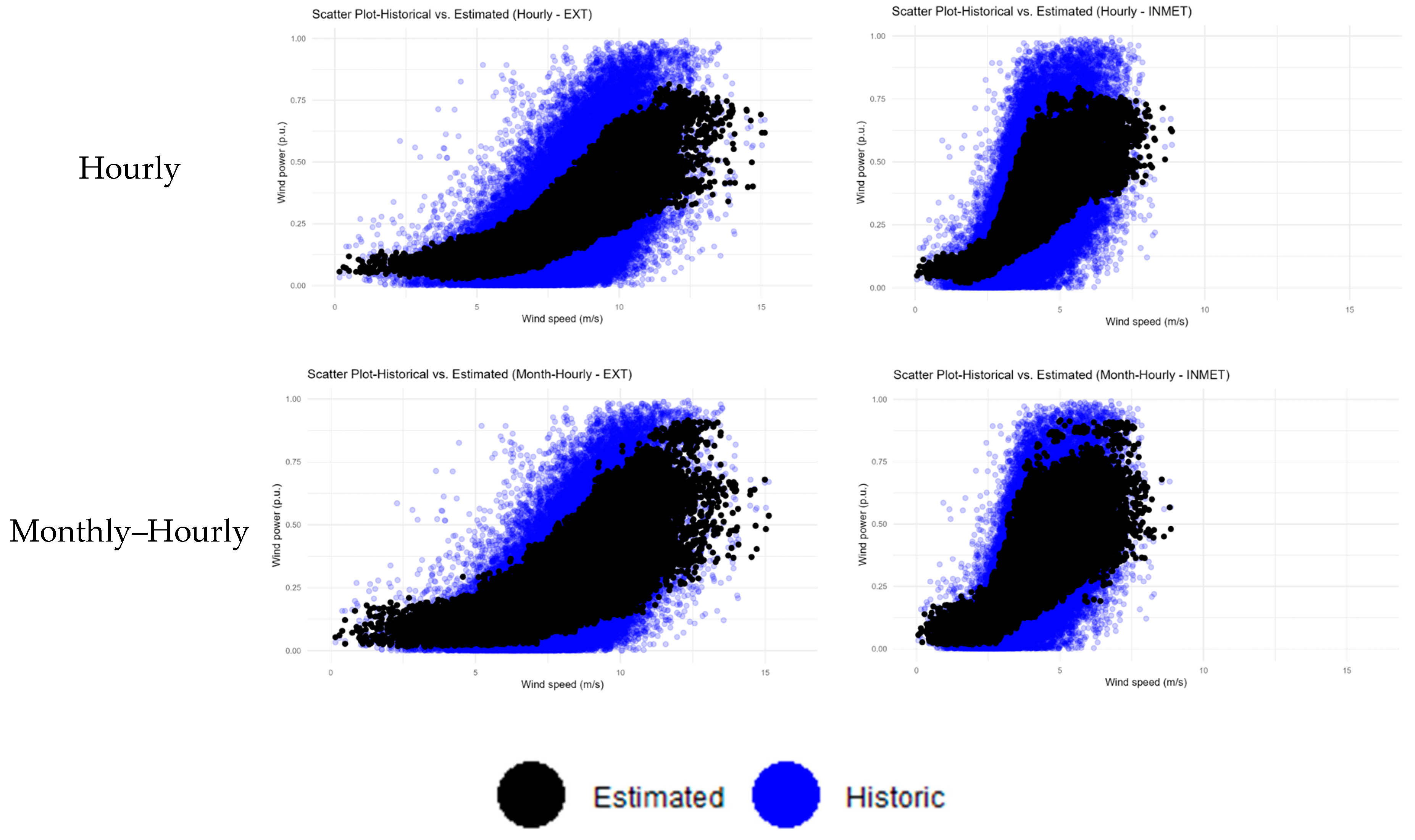
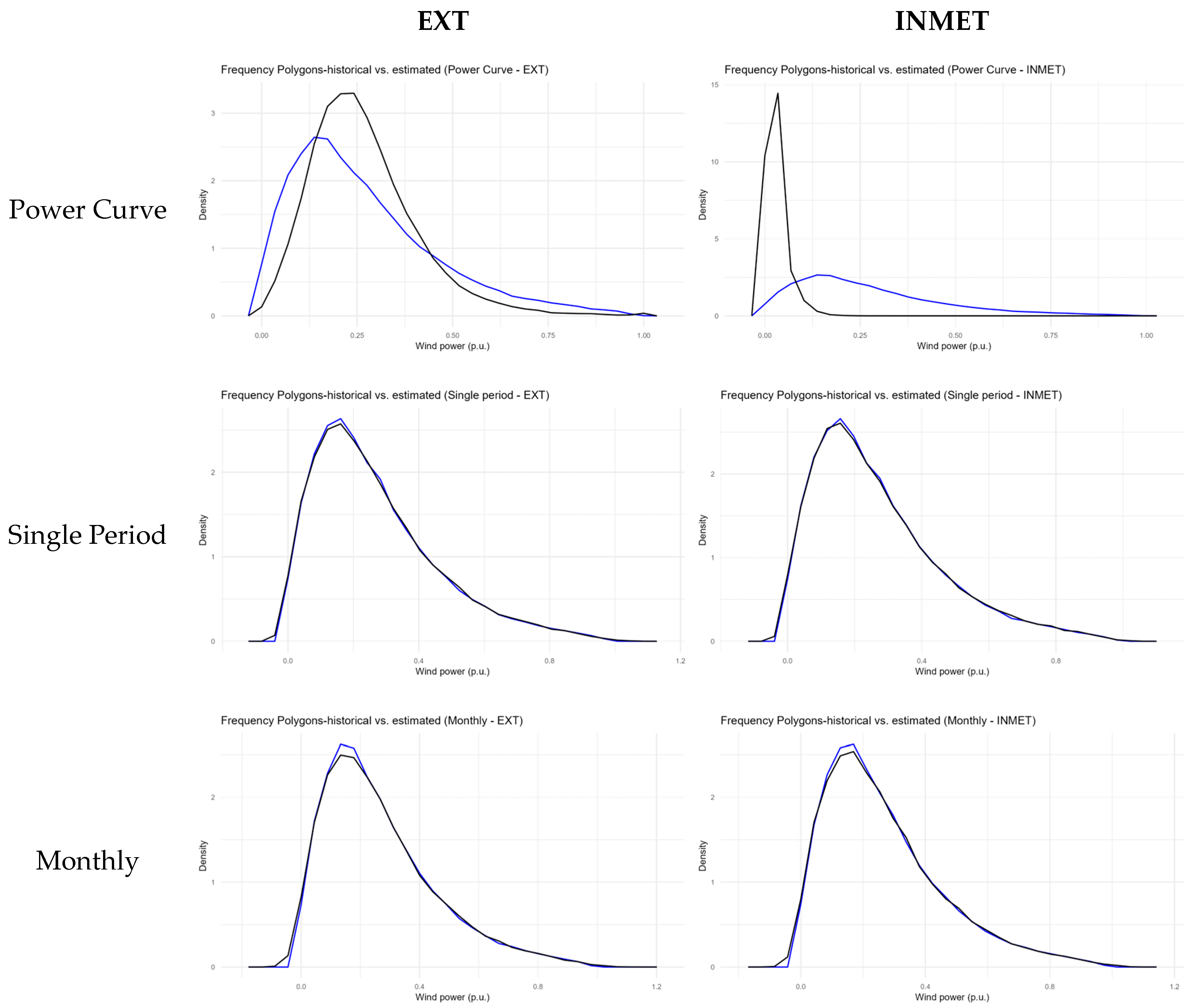
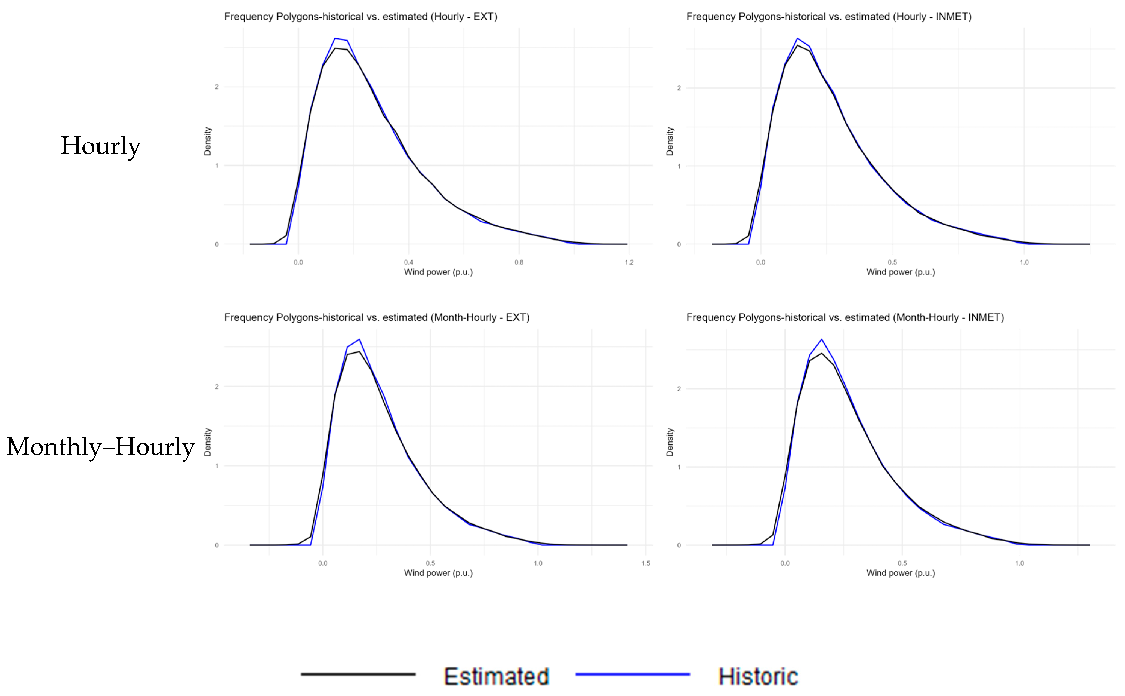
Figure 6 and Figure 7 compare the behavior of the wind farms’ historical data with the estimates resulting from each approach of the proposed method. The blue dots and lines in the graphs refer to historical data, while the black ones denote the estimated values. Figure 6 presents the dispersion graphs, evidencing the behavior of the power variable using the wind speed variable. From these graphs, it is possible to infer that the strategies described in this study managed to better replicate the inherent generation variability for the same speed values, with a highlight on the monthly–hourly proposal, which best captured the existing stochasticity. Figure 7 contains the frequency polygon graphs that estimate the density curve based on the frequencies of the power value intervals. Once again, it can be noted that the suggested strategies (single-period, monthly, hourly and monthly–hourly) replicate the power frequencies obtained from the historical data better than the cubic power curve.

5. Conclusions

Wind speed significantly influences wind power generation, although it is not the sole determining factor. The power curve traditionally represents the relationship between wind speed and power output, often employing the cubic approach. However, this method fails to fully capture the variability in this relationship and necessitates data, such as the air density, turbine height and efficiency factor, which may not always be readily available. Moreover, the theoretical power curve does not entirely reflect the dynamic regions of wind power generation.
To address this limitation, this paper developed a method that replicates wind generation variability based solely on wind speed, without the need for additional data. The approach leverages clustering, probability density function estimation and simulation, making it a probabilistic and nonparametric technique. A key advantage of this proposal is its reliance solely on historical wind power and speed data; however, one downside is its requirement for measured wind generation data, which may be unavailable or limited for new or recently completed wind farms.
This paper utilized historical active wind power data and MERRA-2 reanalysis wind speed data in a study involving five wind farms in Northeast Brazil. The monthly–hourly strategy outperformed the traditional cubic power curve approach.
This new power estimation technique accurately represents power generation variability concerning wind speed, facilitating enhanced project planning and understanding of wind power utilization. It improves data segregation and performance across evaluation criteria by effectively reflecting the probability distribution of historical power production and capturing wind power data characteristics and stochastic behavior.
When accurate wind speed data were challenging to acquire, the proposal turned to the MERRA-2 dataset as a dependable alternative. Two types of wind speed series from MERRA-2 were employed: one with interpolation and extrapolation (EXT) and the other with these steps and bias correction (INMET). Both types yielded favorable results in the four approaches considered. When the performances were compared, they alternated in producing the best results and sometimes even yielded the same results for each evaluation metric. This pattern persisted across all tests, irrespective of the evaluation metric, wind farms and analysis details.
Notably, wind speed data from the INMET station consistently indicated low values, potentially resulting in underestimation after the bias correction step. This impact was observed across all wind farms, including the recommended bias correction sites (Farms 3, 4, and 5). Conversely, the power curve method did not consistently demonstrate complete formation, often leaving the maximum turbine generation unspecified. However, the new method proposed in this article remains unaffected, as all power possibilities derive from occurring wind speeds, effectively addressing the underestimation.
Future endeavors include evaluating this method with other renewable energy sources to ascertain its efficacy, exploring additional clustering and PDF estimation approaches, and considering improved methods for segmenting the data to apply the new method. Furthermore, leveraging a multivariate modeling approach for evaluating other variables from MERRA-2 and wind speed to estimate wind generation warrants consideration.
Supplementary Materials

The supporting information can be downloaded at https://github.com/saulocustodio/Custodio_Cyrino_Macaira_Energies_2024_NewMethod_WindSpeed_Vs_WindPower.git (accessed on 19 May 2024).

Author Contributions

Conceptualization, S.C.d.A.F., P.M.M. and F.L.C.O.; methodology, S.C.d.A.F., P.M.M. and F.L.C.O.; software, S.C.d.A.F. and P.M.M.; validation, S.C.d.A.F., P.M.M. and F.L.C.O.; formal analysis, S.C.d.A.F., P.M.M. and F.L.C.O.; investigation, S.C.d.A.F.; resources, P.M.M. and F.L.C.O.; data curation, S.C.d.A.F.; writing—original draft preparation, S.C.d.A.F.; writing—review and editing, P.M.M. and F.L.C.O.; visualization, S.C.d.A.F.; P.M.M. and F.L.C.O.; funding acquisition, P.M.M. and F.L.C.O. All authors have read and agreed to the published version of the manuscript.

Funding

This work was funded by the Brazilian Coordination for the Improvement of Higher Level Personnel (CAPES) under Grant [number 001]; the Brazilian National Council for Scientific and Technological Development (CNPq-309064/2021-0, 422470/2021-0, 307084/2022-1, 311519/2022-9, 402971/2023-0); and the Carlos Chagas Filho Research Support Foundation of the State of Rio de Janeiro (FAPERJ-202.825/2019, 210.618/2019, 211.086/2019, 211.645/2021, 201.231/2022, 201.243/2022, 201.348/2022, 210.041/2023, 210.015/2024).

Data Availability Statement

The database is available in the Supplementary Material.

Conflicts of Interest

The authors declare no conflicts of interest.

References

  1. Ayodele, T.R.; Ogunjuyigbe, A.S.O. Wind energy resource, wind energy conversion system modelling and integration: A survey. Int. J. Sustain. Energy 2015, 34, 657–671. [Google Scholar] [CrossRef]
  2. Ipakchi, A.; Albuyeh, F. Grid of the future. IEEE Power Energy Mag. 2009, 7, 52–62. [Google Scholar] [CrossRef]
  3. Han, S.; Yang, S.; Liu, Y. The Comparison of BP Network and RBF Network in Wind Power Prediction Application. In Proceedings of the Second International Conference on Bio-Inspired Computing: Theories and Applications, Zhengzhou, China, 14–17 September 2007; pp. 173–176. [Google Scholar] [CrossRef]
  4. Rezvani, A.; Esmaeily, A.; Etaati, H.; Mohammadinodoushan, M. Intelligent hybrid power generation system using new hybrid fuzzy-neural for photovoltaic system and RBFNSM for wind turbine in the grid connected mode. Front. Energy 2019, 13, 131–148. [Google Scholar] [CrossRef]
  5. Fang, D.; Wang, J. A novel application of artificial neural network for wind speed estimation. Int. J. Sustain. Energy 2017, 36, 415–429. [Google Scholar] [CrossRef]
  6. Thapar, V.; Agnihotri, G.; Sethi, V.K. Critical analysis of methods for mathematical modelling of wind turbines. Renew. Energy 2011, 36, 3166–3177. [Google Scholar] [CrossRef]
  7. Carrillo, C.; Obando Montaño, A.F.; Cidrás, J.; Díaz-Dorado, E. Review of power curve modelling for wind turbines. Renew. Sustain. Energy Rev. 2013, 21, 572–581. [Google Scholar] [CrossRef]
  8. Al-Quraan, A.; Al-Masri, H.; Al-Mahmodi, M.; Radaideh, A. Power curve modelling of wind turbines—A comparison study. IET Renew. Power Gener. 2022, 16, 362–374. [Google Scholar] [CrossRef]
  9. Shetty, R.P.; Sathyabhama, A.; Pai, P.S. Comparison of modeling methods for wind power prediction: A critical study. Front. Energy 2020, 14, 347–358. [Google Scholar] [CrossRef]
  10. Shokrzadeh, S.; Jafari Jozani, M.; Bibeau, E. Wind Turbine Power Curve Modeling Using Advanced Parametric and Nonparametric Methods. IEEE Trans. Sustain. Energy 2014, 5, 1262–1269. [Google Scholar] [CrossRef]
  11. Sohoni, V.; Gupta, S.C.; Nema, R.K. A Critical Review on Wind Turbine Power Curve Modelling Techniques and Their Applications in Wind Based Energy Systems. J. Energy 2016, 2016, 8519785. [Google Scholar] [CrossRef]
  12. Wen, J.; Zheng, Y.; Donghan, F. A review on reliability assessment for wind power. Renew. Sustain. Energy Rev. 2009, 13, 2485–2494. [Google Scholar] [CrossRef]
  13. Giorsetto, P.; Utsurogi, K. Development of a New Procedure for Reliability Modeling of Wind Turbine Generators. IEEE Trans. Power Appar. Syst. 1983, PAS-102, 134–143. [Google Scholar] [CrossRef]
  14. Mathew, S. Wind Energy: Fundamentals, Resource Analysis and Economics; Springer: Berlin/Heidelberg, Germany, 2006. [Google Scholar] [CrossRef]
  15. Carta, J.A.; Ramírez, P.; Velázquez, S. A review of wind speed probability distributions used in wind energy analysis. Renew. Sustain. Energy Rev. 2009, 13, 933–955. [Google Scholar] [CrossRef]
  16. Gill, S.; Stephen, B.; Galloway, S. Wind Turbine Condition Assessment Through Power Curve Copula Modeling. IEEE Trans. Sustain. Energy 2012, 3, 94–101. [Google Scholar] [CrossRef]
  17. Wang, Y.; Infield, D.G.; Stephen, B.; Galloway, S.J. Copula-based model for wind turbine power curve outlier rejection. Wind Energy 2014, 17, 1677–1688. [Google Scholar] [CrossRef]
  18. Muralidharan, S.; Parthasarathy, S.; Deepa, A.; Jersha, J. A Comparative Study of Machine Learning Techniques for Wind Turbine Performance Prediction. E3S Web Conf. 2023, 387, 04011. [Google Scholar] [CrossRef]
  19. Kusiak, A.; Zheng, H.; Song, Z. Models for monitoring wind farm power. Renew. Energy 2009, 34, 583–590. [Google Scholar] [CrossRef]
  20. Üstüntaş, T.; Şahin, A.D. Wind turbine power curve estimation based on cluster center fuzzy logic modeling. J. Wind. Eng. Ind. Aerodyn. 2008, 96, 611–620. [Google Scholar] [CrossRef]
  21. Marvuglia, A.; Messineo, A. Monitoring of wind farms’ power curves using machine learning techniques. Appl. Energy 2012, 98, 574–583. [Google Scholar] [CrossRef]
  22. Lydia, M.; Kumar, S.S.; Selvakumar, A.I.; Prem Kumar, G.E. A comprehensive review on wind turbine power curve modeling techniques. Renew. Sustain. Energy Rev. 2014, 30, 452–460. [Google Scholar] [CrossRef]
  23. Duca, V.E.L.A.; Fonseca, T.C.O.; Cyrino Oliveira, F.L. Joint modelling wind speed and power via Bayesian Dynamical models. Energy 2022, 247, 123431. [Google Scholar] [CrossRef]
  24. Lázaro, R.; Yürüşen, N.Y.; Melero, J.J. Wind Turbine Power Curve Modelling using Gaussian Mixture Copula, ANN Regressive and BANN. J. Phys. Conf. Ser. 2022, 2265, 032083. [Google Scholar] [CrossRef]
  25. Wacker, B.; Seebaß, J.V.; Schlüter, J.C. A modular framework for estimating annual averaged power output generation of wind turbines. Energy Convers. Manag. 2020, 221, 113149. [Google Scholar] [CrossRef]
  26. Milad, S.; Milićević, S.; Katić, V.A.; Stanisavljević, A.M. Wind Turbine Modeling Using Wind Speed Measurement Data. In Proceedings of the 22nd International Symposium on Power Electronics (Ee), Novi Sad, Serbia, 25–28 October 2023; pp. 1–5. [Google Scholar] [CrossRef]
  27. Jung, C.; Schindler, D. Wind speed distribution selection—A review of recent development and progress. Renew. Sustain. Energy Rev. 2019, 114, 109290. [Google Scholar] [CrossRef]
  28. Khodabux, K.; Bhujun, B.S.; Naidu, R.C.; Busawon, K. Mathematical approach to modelling sigmoidal power curves for Wind Energy Conversion Systems. In Proceedings of the 7th International Conference on Environment Friendly Energies and Applications (EFEA), Bagatelle Moka MU, Mauritius, 14–16 December 2022; pp. 1–6. [Google Scholar] [CrossRef]
  29. De Aquino Ferreira, S.C.; Cyrino Oliveira, F.L.; Maçaira, P.M. Validation of the representativeness of wind speed time series obtained from reanalysis data for Brazilian territory. Energy 2022, 258, 124746. [Google Scholar] [CrossRef]
  30. SIGEL ANEEL—Sistema de Informações Georreferenciadas do Setor Elétrico da Agência Nacional de Energia Elétrica. Available online: https://sigel.aneel.gov.br/portal/home/ (accessed on 9 April 2023).
  31. The Wind Power. Available online: https://www.thewindpower.net/(accessed on 10 January 2024).
  32. Gruber, K.; Klöckl, C.; Regner, P.; Baumgartner, J.; Schmidt, J. Assessing the Global Wind Atlas and local measurements for bias correction of wind power generation simulated from MERRA-2 in Brazil. Energy 2019, 189, 116212. [Google Scholar] [CrossRef]
  33. Dos Santos, F.S.; Do Nascimento, K.K.F.; Da Silva Jale, J.; Xavier, S.F.A.; Ferreira, T.A.E. Brazilian wind energy generation potential using mixtures of Weibull distributions. Renew. Sustain. Energy Rev. 2024, 189, 113990. [Google Scholar] [CrossRef]
  34. Global Modeling and Assimilation Office (GMAO): Modern-Era Retrospective Analysis for Research and Applications. National Aeronatuics and Space Administration. Available online: https://gmao.gsfc.nasa.gov/reanalysis/MERRA-2/ (accessed on 21 May 2021).
  35. Celebi, M.E.; Kingravi, H.A.; Vela, P.A. A comparative study of efficient initialization methods for the k-means clustering algorithm. Expert Syst. Appl. 2013, 40, 200–210. [Google Scholar] [CrossRef]
  36. Esteves, G.; Maçaira, P.; Oliveira, F.; Amador, G.; Souza, R. Improvements in the Current Brazil’s Energy Dispatch Optimization: Load Forecast and Wind Power. In Proceedings of the 8th International Conference on Operations Research and Enterprise Systems, Prague, Czech Republic, 19–21 February 2019; pp. 398–405. [Google Scholar] [CrossRef]
  37. Li, H.; Yu, Y.; Huang, Z.; Sun, S.; Jia, X. A multi-step ahead point-interval forecasting system for hourly PM2.5 concentrations based on multivariate decomposition and kernel density estimation. Expert Syst. Appl. 2023, 226, 120140. [Google Scholar] [CrossRef]
  38. Wahbah, M.; Feng, S.F.; EL-Fouly, T.H.M.; Zahawi, B. Wind speed probability density estimation using root-transformed local linear regression. Energy Convers. Manag. 2019, 199, 111889. [Google Scholar] [CrossRef]
  39. Worton, B.J. Using Monte Carlo Simulation to Evaluate Kernel-Based Home Range Estimators. J. Wildl. Manag. 1995, 59, 794. [Google Scholar] [CrossRef]
  40. Van Ravenzwaaij, D.; Cassey, P.; Brown, S.D. A simple introduction to Markov Chain Monte–Carlo sampling. Psychon. Bull. Rev. 2018, 25, 143–154. [Google Scholar] [CrossRef] [PubMed]
  41. MacQueen, J. Some methods for classification and analysis of multivariate observations. In Proceedings of the Fifth Berkeley Symposium on Mathematical Statistics and Probability; University of California Press: Berkeley, CA, USA, 1967; pp. 281–297. [Google Scholar]
  42. Duca, V.E.L.A.; Fonseca, T.C.O.; Cyrino Oliveira, F.L. An overview of non-Gaussian state-space models for wind speed data. Energy 2023, 266, 126436. [Google Scholar] [CrossRef]
  43. Al-Duais, F.S.; Al-Sharpi, R.S. A unique Markov chain Monte Carlo method for forecasting wind power utilizing time series model. Alex. Eng. J. 2023, 74, 51–63. [Google Scholar] [CrossRef]
  44. Wang, Y.; Hu, Q.; Li, L.; Foley, A.M.; Srinivasan, D. Approaches to wind power curve modeling: A review and discussion. Renew. Sustain. Energy Rev. 2019, 116, 109422. [Google Scholar] [CrossRef]
  45. R Core Team—A Language and Environment for Statistical Computing. Available online: https://www.r-project.org/ (accessed on 21 December 2023).
  46. Silva, G.R. Características de Vento da Região Nordeste—Análise, Modelagem e Aplicações para Projetos de Centrais Eólicas. Master’s Thesis, Universidade Federal de Pernambuco, Recife, Brazil, 2003. [Google Scholar]
Figure 1. Steps of the method.
Energies 17 03573 g001
Figure 2. Comparison of wind power behavior between wind farms. (a) Wind farm probability density functions. (b) Variability of wind power provided by wind farms.
Energies 17 03573 g002
Figure 3. Boxplot of the wind power data per (a) hour and (b) month.
Energies 17 03573 g003aEnergies 17 03573 g003b
Figure 4. Results of clustering (Wind Farm 5). (a) Result of applying the elbow method; (b) scatterplot of wind speed and power identified by cluster.
Energies 17 03573 g004
Figure 5. Evolution of the shape of the power probability density curve based on increasing wind speed values (Wind Farm 5).
Energies 17 03573 g005aEnergies 17 03573 g005b
Figure 6. Dispersion graphs that compare how much the estimated data replicate the historical data by treatment (Wind Farm 5).
Energies 17 03573 g006aEnergies 17 03573 g006b
Figure 7. Polygon graphs of the estimated and historic frequency data (Wind Farm 5).
Energies 17 03573 g007aEnergies 17 03573 g007b
Table 1. Information about the wind farms.
Wind FarmLocation in the StateInstalled Capacity (KW)Number of TurbinesTotal Wind Turbine Height (m)Rotor Diameter (m)Operating Period
1Interior31,50015194.00114.001 November 2017 to 28 February 2022
2Interior63,00030194.00114.00
3Coast10,2001398.8548.001 January 2013 to 28 February 2022
4Coast48,0006099.6048.00
5Coast45003123.5077.00
Table 2. Turbine models on the wind farms.
Wind FarmManufacturerModelRotor Diameter (m) v c i (m/s) v r (m/s) v c o (m/s) C p , m a x
1Gamesa (Spain)G114/21001143.510250.45
2Gamesa (Spain)G114/21001143.510250.45
3Enercon (Brazil)E48/80048314250.50
4Enercon (Brazil)E48/80048314250.50
5IMPSAr (Argentina)IV-77-150077313220.42
Table 3. Data from adjusting the wind speed data from MERRA-2.
Wind FarmHub Height (m)Distance
MERRA-2—Wind Farm (km)INMET—Wind Farm (km)
1137.0018.6452.97
2137.0014.9554.65
374.853.4119.86
475.609.0117.92
585.007.6113.49
Table 4. Number of clusters obtained using each approach.
Wind FarmSpeed TreatmentApproaches of the Proposed Method
SingularMonthlyHourlyMonthly–Hourly
1EXT2318–2212–203–12
INMET2017–2217–203–11
2EXT2017–2115–205–12
INMET2018–2216–205–12
3EXT2118–2214–206–12
INMET2218–2115–205–10
4EXT2218–2213–206–12
INMET2117–2213–195–12
5EXT2218–2212–195–12
INMET2218–2212–206–12
Table 5. Results reached by the methods according to the evaluation metrics.
MetricsWind FarmSpeed TreatmentMethods
Cubic Power CurveProposals
SingularMonthlyHourlyMonthly–Hourly
RMSE1EXT0.60120.23150.22100.20290.1772
INMET0.44890.24280.23100.20320.1771
2EXT0.59710.20090.18920.17750.1538
INMET0.32240.21030.19420.17780.1538
3EXT0.16240.15970.15460.15590.1454
INMET0.34390.17130.16400.15590.1455
4EXT0.15900.14440.13850.13720.1249
INMET0.28040.14820.14160.13730.1248
5EXT0.25900.15800.15370.13300.1245
INMET0.27670.15360.14940.13300.1247
MAE1EXT0.45290.18830.17840.15780.1349
INMET0.36970.19980.18840.15810.1347
2EXT0.44490.16150.15090.13820.1179
INMET0.25540.17070.15570.13850.1180
3EXT0.12450.12450.12010.12060.1112
INMET0.28260.13430.12760.12060.1113
4EXT0.12090.11180.10600.10500.0930
INMET0.22260.11420.10740.10510.0930
5EXT0.20640.12300.11860.10180.0949
INMET0.22090.11770.11400.10190.0950
MAPE1EXT0.46480.19320.18310.16200.1384
INMET0.37940.20500.19340.16230.1383
2EXT0.46690.16950.15840.14510.1238
INMET0.26810.17920.16340.14530.1239
3EXT0.12490.12490.12050.12100.1115
INMET0.28340.13470.12800.12100.1117
4EXT0.12790.11830.11220.11120.0984
INMET0.23560.12090.11370.11130.0984
5EXT0.20770.12380.11940.10250.0955
INMET0.22230.11840.11480.10250.0956
R21EXT−2.81840.43380.48400.56500.6682
INMET−1.12940.37690.43640.56370.6687
2EXT−3.55600.48420.54260.59720.6979
INMET−0.32800.43480.51830.59610.6978
3EXT0.42010.43870.47440.46570.5351
INMET−1.60190.35420.40830.46510.5343
4EXT0.28890.41390.46030.47040.5616
INMET−1.21020.38250.43650.46960.5619
5EXT−0.87260.30290.34050.50630.5673
INMET−1.13780.34160.37720.50610.5660
Table 6. RMSEs attained by the methods per month.
Wind FarmMethodsSpeed TreatmentMonths
JanFebMarAprMayJunJulAugSepOctNovDec
1Theoretical CurveEXT0.52980.47160.45960.47210.52400.55090.54970.69390.76110.74470.71190.6194
INMET0.37770.32040.31330.35490.43590.51880.54720.56630.53030.46450.45220.4353
SingularEXT0.23760.23270.24390.23450.22060.22880.22120.20980.20870.23280.25180.2426
INMET0.24770.24050.25400.23910.22800.23690.23260.22610.22310.24760.26550.2586
MonthlyEXT0.23050.21450.22380.22380.21770.21650.19750.18420.19990.23200.24980.2398
INMET0.23990.22110.22830.22720.22460.22590.20910.19740.21020.24670.26230.2548
HourlyEXT0.21520.22080.23600.22660.21040.20840.20260.17450.15820.17750.19170.1993
INMET0.21460.22150.23690.22700.21040.20810.20290.17550.15900.17750.19230.1998
Monthly–HourlyEXT0.20270.19960.20280.20200.19380.18070.16080.13610.13820.14780.16020.1779
INMET0.20340.19850.20250.20270.19310.18090.16000.13610.13840.14630.15980.1785
2Theoretical CurveEXT0.51110.46430.44940.47430.54280.55400.56200.71540.77350.73220.68500.5895
INMET0.28570.24410.23820.27160.31490.36450.37920.38120.35610.33740.33680.3241
SingularEXT0.20230.20070.21500.20750.19710.19720.19500.20180.18820.19310.20840.2019
INMET0.20920.21820.23670.22830.22030.21330.20700.20760.19130.19240.20080.1998
MonthlyEXT0.19720.18100.18770.18690.19000.18910.17640.17630.17750.19210.20590.1998
INMET0.20070.18810.19460.20020.21070.20640.18990.17310.17440.18860.19780.1992
HourlyEXT0.18170.18670.20450.19660.18970.18310.18180.17310.14880.14930.16060.1705
INMET0.18150.18800.20550.19740.19080.18240.18210.17260.14880.15010.16060.1699
Monthly–HourlyEXT0.17420.16440.17250.16500.16760.16060.14860.13760.12900.12270.13660.1536
INMET0.17390.16480.17220.16540.16850.16080.14880.13750.12990.12330.13490.1533
3Theoretical CurveEXT0.13680.13440.12850.14380.15880.19330.21390.19810.18510.15680.13900.1327
INMET0.29740.28750.24440.25340.25880.32780.37360.42920.45220.42960.36350.3277
SingularEXT0.13520.13440.12870.14330.15950.18950.19870.19480.18340.15720.13850.1320
INMET0.14340.14300.13500.14640.15840.18840.19850.19750.20810.19120.17180.1560
MonthlyEXT0.13350.13210.12840.14200.15040.17960.19010.19260.18030.14720.12990.1284
INMET0.14170.14110.12980.14060.14410.18160.19570.19000.19510.17770.16330.1506
HourlyEXT0.12960.12820.11980.13650.15270.18560.19500.18700.18080.15830.14210.1329
INMET0.13020.12780.11950.13610.15260.18570.19530.18680.18120.15880.14180.1334
Monthly–HourlyEXT0.12540.12460.11790.13240.13690.17010.18190.17830.17540.14100.11860.1199
INMET0.12500.12470.11810.13360.13730.16950.18280.17870.17470.14130.11860.1199
4Theoretical CurveEXT0.12060.11650.11700.13870.16400.20440.23500.20870.17670.13930.11390.1115
INMET0.24680.23520.19850.20080.20400.25730.29660.35510.37550.35570.29410.2683
SingularEXT0.12240.11830.11230.12690.14110.16860.18520.18340.16920.14390.11860.1155
INMET0.12470.12190.11260.12180.13210.15830.17240.17500.18380.17110.14770.1360
MonthlyEXT0.11920.11490.11190.12550.13270.15730.17510.18090.16530.13370.10990.1101
INMET0.12330.12090.11010.11690.11980.14980.16730.16960.17440.15860.13970.1290
HourlyEXT0.11780.11210.10240.11570.12800.15610.16770.16250.16460.14920.12990.1213
INMET0.11770.11200.10230.11590.12840.15620.16870.16220.16450.14940.12970.1212
Monthly–HourlyEXT0.11140.10810.10130.11160.11140.13620.15200.15250.15820.12980.10230.1045
INMET0.11160.10840.10120.11160.11130.13630.15130.15280.15770.12970.10270.1044
5Theoretical CurveEXT0.19560.18430.18490.21500.25150.32000.35680.33490.32370.26090.19570.1915
INMET0.25310.24600.20600.19900.21060.25410.29200.35390.34000.33650.29650.2707
SingularEXT0.14700.14250.13200.13580.14590.16500.18380.19590.18670.16630.14080.1359
INMET0.13610.13260.12390.12770.13840.15620.17240.18780.18130.17260.15360.1420
MonthlyEXT0.14540.13970.12990.13240.13840.15760.17820.19280.18610.16090.13100.1316
INMET0.13520.13210.12100.12140.12860.15090.17020.18180.17910.16640.14740.1390
HourlyEXT0.12670.11900.11110.11360.12430.14510.15210.14770.14740.14100.13250.1261
INMET0.12720.11930.11130.11380.12410.14460.15210.14820.14730.14060.13220.1261
Monthly–HourlyEXT0.12240.11590.10880.10770.11220.13160.14480.13880.14280.13000.11390.1160
INMET0.12290.11580.10870.10890.11250.13120.14450.13910.14330.12970.11420.1164
The best result for each wind farm is shown in bold.
Table 7. RMSEs attained by the methods per hour.
Wind FarmMethodsSpeed TreatmentHours
123456789101112131415161718192021222324
1Theoretical CurveEXT0.85850.76800.66710.56370.49180.45000.41540.38560.36570.56350.78240.71390.59530.48510.39980.33630.30790.32440.38170.44100.71880.86980.89720.8661
INMET0.43740.43930.44260.45110.45590.45540.46790.50260.49890.47090.38220.28620.22120.20010.21610.25780.32070.40250.55090.65630.63240.59780.53770.4630
SingularEXT0.25260.24480.23420.22490.22160.21780.21230.22010.21510.20730.22690.23400.21300.18610.16400.15220.16990.21330.31100.34770.25460.24500.24670.2501
INMET0.26220.25650.24400.22960.22420.21810.20980.21970.21670.23070.17030.19510.23540.23570.21320.18250.17080.20900.31940.39650.30240.26690.24830.2516
MonthlyEXT0.22900.22160.21380.20890.20980.20590.20220.20650.20160.19330.21810.23470.21960.19810.17690.16230.16840.20550.29660.33550.25040.22540.22240.2246
INMET0.23000.22870.22120.21280.21270.20690.19980.20430.20120.21060.16820.20170.24060.24310.22600.19370.17820.20100.29810.37290.29090.25100.22910.2240
HourlyEXT0.25010.24350.22970.22180.21580.21280.20320.20210.19570.20440.15490.13190.12030.11670.12590.14010.16690.19580.22370.23710.22920.23980.24630.2471
INMET0.24950.24150.23020.22130.21700.21240.20340.20310.19680.20620.15530.13320.11880.11840.12650.14090.16760.19570.22520.23670.23120.23890.24610.2477
Monthly–HourlyEXT0.20750.19990.19790.19480.19800.19600.19050.18360.18060.16350.14290.12700.11680.11350.12440.13690.15710.17830.18860.18080.18110.20200.21270.2130
INMET0.20640.19850.19750.19480.19840.19650.19040.18420.17870.16500.14110.12620.11660.11260.12270.13700.15930.17880.18960.18170.18260.20370.21140.2099
2Theoretical CurveEXT0.84310.74590.64140.53480.45590.40940.38610.37280.36060.55460.76660.69520.57660.46570.38560.32730.29760.31450.36420.43650.78750.92660.92390.8679
INMET0.25620.24190.27590.31810.35590.40080.43650.47700.48740.45400.33400.23970.17880.15090.15450.19730.24590.30410.37440.39110.27300.27980.24230.3135
SingularEXT0.19930.19230.18290.17810.17950.18390.19010.20910.21300.19860.20910.22080.20110.17420.15360.14990.16430.20340.25900.26900.22270.21430.20660.2006
INMET0.21870.21110.20010.19070.18750.19670.21520.24910.26510.26390.17550.17540.19060.19860.19060.17540.17340.18760.22330.23670.22340.22610.21310.2184
MonthlyEXT0.18130.17650.17150.16700.16900.17240.17690.19560.20040.19730.20910.22240.20780.18430.16420.15240.15620.18480.23980.25210.19630.17790.17360.1738
INMET0.18990.18930.18240.17640.17160.17950.19690.22880.24520.23910.17200.18050.19890.20630.20020.18080.16990.17920.21150.21900.18160.17790.17460.1804
HourlyEXT0.19540.18690.17680.17110.16750.17150.17470.18630.18690.19670.16080.13780.12230.11750.12140.14340.16340.18520.20620.21430.21440.20870.20010.1939
INMET0.19420.18780.17760.17160.16770.17100.17540.18690.18820.19720.16050.13860.12200.11690.12110.14250.16280.18510.20740.21590.21410.21000.19960.1938
Monthly–HourlyEXT0.16430.15780.15480.15410.15340.15870.15970.17100.17440.16840.15030.13340.12110.11480.11600.13360.14530.15870.16530.15730.15870.16660.16460.1650
INMET0.16270.15670.15570.15450.15190.15760.16100.17090.17390.16780.15000.13210.12180.11440.11720.13260.14670.15850.16630.15880.15860.16700.16640.1650
3Theoretical CurveEXT0.15580.15800.16230.16590.16770.17150.17570.18310.17020.14110.13000.13770.14740.15390.16240.16620.16870.17010.16860.16980.16790.16760.16380.1606
INMET0.33680.32880.32620.32690.32580.32680.31560.29980.30600.31930.33160.33750.33970.34340.35120.35680.36200.36780.36880.37880.38470.38200.36720.3502
SingularEXT0.15760.15970.16420.16660.16870.17230.17780.18540.17290.14380.13090.13410.13970.14580.15370.15800.15920.16050.15700.16220.16360.16540.16200.1605
INMET0.16570.16530.16970.17460.17550.17800.17560.17760.17160.16250.15530.16220.16520.17250.17900.18070.17900.17400.16580.16510.17310.17700.17440.1701
MonthlyEXT0.14570.15080.15560.15960.16050.16490.16730.17190.16020.14030.13530.13810.14530.14970.15730.16060.16010.16040.15530.15670.15560.15430.15030.1482
INMET0.15390.15510.16020.16540.16580.16760.16510.16310.15700.15470.15320.16450.16760.17060.17270.17390.17120.16650.15920.16400.17360.16830.16210.1580
HourlyEXT0.15580.15820.16160.16530.16670.17040.17140.17120.16270.13900.12900.13320.13910.14550.15310.15570.15570.15480.15080.15350.15700.15960.16120.1605
INMET0.15620.15810.16220.16470.16660.17010.17140.17230.16380.13910.12890.13260.14010.14530.15250.15500.15490.15450.15080.15430.15750.16050.16140.1600
Monthly–HourlyEXT0.14220.14470.14980.15560.15450.15960.15660.15130.14230.13290.12600.13020.13550.14130.14730.15080.15100.14940.14370.14410.14490.14390.14250.1436
INMET0.14360.14480.15030.15610.15520.15820.15760.14990.14290.13290.12620.13030.13700.14100.14760.15010.15030.14950.14410.14530.14440.14390.14170.1438
4Theoretical CurveEXT0.15820.16130.16550.16860.17270.17710.18790.19280.16380.12700.12350.13240.14320.14700.15350.15290.15710.16120.16450.16430.15700.15590.15470.1557
INMET0.25180.24060.23740.23480.23160.23100.22980.23420.25460.28560.30450.31020.31160.31110.31270.31390.31210.30810.29880.30170.30580.30350.28710.2678
SingularEXT0.14050.14100.14370.14530.14720.15030.15880.16320.14260.12740.12540.12700.13650.14030.14740.14950.15040.14940.14450.14770.14570.14830.14500.1419
INMET0.13800.13600.13840.13890.13830.14000.14560.15180.14460.15830.15590.14960.14780.15000.15520.15810.15870.15680.14990.14770.14760.15270.14950.1428
MonthlyEXT0.12510.12710.13190.13490.13570.13810.14620.14900.12870.12750.13120.13390.14140.14580.15270.15380.15270.14940.14140.14220.13670.13600.13010.1268
INMET0.12570.12390.12580.12720.12670.12760.13180.13730.13010.15440.15570.15190.15160.15000.15290.15250.15430.15110.14700.14850.14760.14540.13710.1300
HourlyEXT0.13600.13470.13690.13720.13760.13810.14410.14820.13670.12160.11950.12290.13110.13550.14070.14170.14220.14200.13780.13960.14000.14400.14220.1393
INMET0.13590.13450.13690.13760.13740.13830.14330.14780.13750.12230.11940.12340.13080.13490.14120.14060.14230.14220.13790.14010.14010.14440.14320.1397
Monthly–HourlyEXT0.11690.11650.11940.12270.12050.12130.12550.12550.11870.11780.11620.12030.12730.13020.13510.13630.13710.13570.12840.12890.12570.12560.12160.1193
INMET0.11700.11590.12050.12240.12000.12160.12520.12650.11830.11680.11540.12070.12710.12990.13570.13590.13750.13620.12880.12900.12530.12440.12180.1193
5Theoretical CurveEXT0.27850.27990.28230.28500.29340.30190.31550.30850.24800.17400.17180.18690.19660.20230.20930.21770.23910.27720.29390.28660.28130.26890.26770.2706
INMET0.20360.19630.19510.19340.19020.18870.19410.22770.29220.35600.38220.38760.38690.37900.36680.34400.29320.23600.21770.22790.24080.24400.23010.2151
SingularEXT0.12970.13200.13570.13600.13980.14250.15410.16360.15600.17610.18640.19560.20550.21150.20980.19590.16220.13560.12960.12710.12530.12340.12200.1245
INMET0.11120.11230.11130.10940.10900.11140.12440.14550.16670.21820.21970.20170.19070.18370.17890.17120.16150.16820.16460.14690.12480.11730.11320.1122
MonthlyEXT0.12290.12560.13100.13360.13560.13880.14750.15050.14340.17030.18440.19310.20240.20920.20650.19510.15870.13300.12800.12630.12310.11900.11570.1168
INMET0.10680.10870.10860.10710.10730.10930.11830.13290.15270.21050.21340.19720.18860.18230.17600.16730.15590.16190.16080.14830.12870.11610.10910.1074
HourlyEXT0.10770.10650.10840.10730.10660.10710.11900.14350.15510.15060.14670.15290.15880.16480.16740.16570.15080.13170.12010.11900.11700.11600.11180.1086
INMET0.10740.10670.10830.10700.10660.10710.11880.14380.15530.14990.14680.15350.15840.16490.16860.16520.15080.13210.11970.11870.11700.11640.11210.1084
Monthly–HourlyEXT0.09990.10000.10280.10180.10070.10170.10650.11890.12960.14080.14190.14700.15230.15860.16010.15830.14270.12490.11390.11340.11000.10900.10400.1001
INMET0.10050.10010.10260.10240.10020.10140.10660.11920.12980.14100.14170.14750.15420.15870.15900.15900.14360.12480.11380.11270.11040.10870.10420.1011
The best result for each wind farm is shown in bold.
Disclaimer/Publisher’s Note: The statements, opinions and data contained in all publications are solely those of the individual author(s) and contributor(s) and not of MDPI and/or the editor(s). MDPI and/or the editor(s) disclaim responsibility for any injury to people or property resulting from any ideas, methods, instructions or products referred to in the content.