Article

Multiple-Indicator Filtering-Based Information Interaction Evaluation Method of Automatic Distribution Master Station for Grid Security

1
NARI Group Co., Ltd., Nanjing 210037, China
2
NARI-TECH Nanjing Control Systems Co., Ltd., Nanjing 211106, China
3
Power Dispatching and Control Center of Guangdong Power Grid Co., Ltd., Guangzhou 510060, China
*
Author to whom correspondence should be addressed.
Energies 2024, 17(14), 3552; https://doi.org/10.3390/en17143552
Submission received: 28 May 2024 / Revised: 15 July 2024 / Accepted: 16 July 2024 / Published: 19 July 2024

Abstract

:
Automatic distribution master stations (ADMSs) are software platforms that can be used to monitor energy supply and consumption of power demand-side resources as well as to guarantee grid security. They play a vital role in maintaining the optimal performance and stability of electrical power systems. However, the stability of ADMSs is usually determined by the performance of the information interaction, which includes various challenges and complexities. Therefore, an efficient multiple-indicator filtering-based information interaction evaluation method for the ADMS is proposed in this paper. The proposed method first utilizes the principal component analysis (PCA) to filter the indicators of the ADMS. Then, the data envelopment method and the analytic network process (ANP) are employed to remove the invalid indicators and to determine the indicator weights. In this regard, the secondary screening of the indicators is completed, the effective indicators are obtained, and the accuracy of the evaluation system is improved. Results of the simulation show that the proposed method works well when evaluating information interaction performance, and it offers satisfactory performance evaluation of ADMSs.

1. Introduction

In the era of digitization and artificial intelligence, the automatic distribution master stations (ADMSs) are playing an increasingly important role in modern power systems. ADMSs offer solutions to improve the reliability, safety, and flexibility of the power grid. Furthermore, they help to monitor energy supply and consumption of power demand-side resources and guarantee grid security [1,2,3,4]. ADMSs can provide accurate information and data support through information interaction in a timely manner. Moreover, they ensure the efficient, safe, and reliable operation of the modern power system by adapting to the constantly changing energy market and user needs [5,6].
As shown in Figure 1 [7], the system network architecture includes a front-end data collection server with a historical data services device, a supervisory control and data acquisition (SCADA) server, an image data server, an antivirus server, and a web server. At present, the main station of the distribution automation system is divided into two major areas: the first is to monitor the operation of the Zone I distribution network, and the second is to control the operation status of the Zone III distribution network. Zone I mainly realizes functions such as data collection, operation and control, topology analysis, and feeder automation of the distribution network. Zone III mainly realizes functions such as distribution network trend analysis, distribution terminal management, information sharing, and publishing. Two dedicated network data collection servers are used to complete the collection and processing of dedicated network channel data. Two historical data servers are configured in the system to achieve historical data management functions. The system is configured with two SCADA servers, which are connected to a dual network via Gigabit Ethernet to form a dual host and backup mode. This configuration aims to achieve a dual network and dual machine processing architecture. In the system network architecture, a PC server is regarded as an image data server in the automated distribution system to complete the input and maintenance services of the equipment graphics, attribute data, etc. The antivirus server adopts a PC server to complete the antivirus monitoring of the real-time system, image data, and reporting system in Zone I, which ensures the immunity of the system against viruses without affecting its operation. Two PC servers are used as web servers to complete historical data management and web browsing services in the Zone III distribution network. The web server is connected to the backbone network through physical isolation devices and connected to Zone III by a firewall to ensure system security. A PC workstation is also employed as a report workstation to design, view, and print data statistics reports. Furthermore, the coordination and maintenance workstations adopt a single machine dual screen mode to serve various tasks. They aim to achieve control operator monitoring, to control the operation status and opening/closing operations of various equipment in the distribution network, and to complete various human–machine interaction functions. Finally, the graphics workstation uses a PC workstation with excellent graphic processing capabilities to input and maintain device graphics and attribute data [8,9].
The stable and secure information interaction is greatly significant for improving the efficiency of ADMS operations. A reliable information interaction capability can ensure the safe and reliable power supply of the system, which is crucial for ensuring the stable operation of the power systems. To evaluate the information interaction performance of ADMS operation, various scholars have been conducting related research in the past few years. For example, Heydt [10] summarized various concepts of next-generation distribution systems. The goal was to align distribution engineering more closely with the concept of smart grids. Moreover, with the development of new system theory and components/materials, the design, operation, and control issues were discussed. Based on the concept of distribution networks summarized by Heydt, Pirouzi [11] combined effective planning of distributed generation and distribution automation in the distribution network, to improve reliability and operational indicators. Based on the mixed planning method of distributed photovoltaic and photovoltaic master stations, Kazemi [12] further proposed a quantitative analysis method for the adequacy of a specific automated distribution scheme. The reliability of the distribution master station was improved by accelerating the isolation of faulty sections and the recovery of healthy sections. Chen [13] proposed a parallel processing mechanism and overall testing method for distributed SCADA based on the principle of distributed master station model-sharing technology and predistributed acquisition structure. Based on the existing technology research of the distribution main station, Tallon-Ballesteros [14] introduced the information scheme for the safety of the distribution main station. The proposed scheme analyzed the safety of the power transmission data interaction method between the main station and the terminal. In addition, a combination of symmetric and asymmetric algorithms was used to establish a secure link between the main station and the terminal to protect the safety of the main station and the terminal. Yue [15] also proposed a deep integration information interaction evaluation method of ADMSs based on the distribution network automation construction to achieve a decentralized control and centralized processing as well as to improve the interaction efficiency of distribution network automation. In response to the technical research, safety, and interactivity issues of the distribution main station, Ding [16] constructed an evaluation index system and introduced the network analysis method to obtain the weight of the system index, thus obtaining the key indicators that play a leading role in the ADMS. From the above analysis, it can be seen that some scholars have evaluated information interaction performance in ADMSs, e.g., the fusion method of symmetric and asymmetric algorithms [14] and the network analysis method [16]. However, some traditional methods, such as the analytical hierarchy process (AHP) [9], show redundancy when processing evaluation indicators, which leads to unsatisfactory evaluation performance. Therefore, a multiple-indicator filtering-based evaluation method is proposed to effectively evaluate the information interaction performance in ADMSs. In the proposed method, the indicator refining process is developed to purify those evaluation indicators, and is used in the performance evaluation process. Also, the analytic network process (ANP) is utilized to evaluate the information interaction performance in the ADMSs. Therefore, the main contributions are summarized as follows:
  • Some potential indicators, such as the safety indicators, the reliability indicators, the accuracy indicators, and the timelines indicators, are summarized and analyzed in detail to evaluate the information interaction performance in the ADMSs.
  • The proposed evaluation method is introduced and explained, and its computation processes are explained in detail, including the indicator refining process and the performance evaluation process.
  • Extensive evaluations of the proposed evaluation method are implemented and discussed in detail. The simulation results indicate the efficiency of the proposed evaluation method when solving the problem of information interaction performance of the ADMSs.
The rest of this paper is structured as follows: (i) The evaluation indicators of the ADMS are introduced in Section 2; (ii) Section 3 and Section 4 introduce the proposed evaluation method in detail; (iii) The evaluation results are presented and analyzed in Section 5; (v) Finally, concluding remarks are given in Section 6.

2. Evaluation Indicators of the ADMS

ADMSs are usually connected to the actual hardware equipment of the distribution systems. Those various servers in the ADMS can offer some operating status data, namely the current, voltage, power, load situation, etc., which show the actual operating status and performance of the ADMS. By obtaining the operating status data, real information interaction data, such as the safety, reliability, accuracy, and timeliness indicators in the ADMS, can be obtained. Moreover, by analyzing these key aspects, a comprehensive evaluation indicator system is constructed to ensure the accurate evaluation of the information interaction performance of the ADMS. Within the process of constructing the evaluation indicator system, the correlation between various indicators in the ADMS is shown in Figure 1. This evaluation indicator system not only comprehensively reflects the interactive performance of the ADMS information through the area but also provides accurate data support for operators. Hence, the evaluation indicator system ensures that the ADMSs can effectively manage and maintain the daily safe operation of the distribution system.

2.1. Safety Indicator A

Data security interaction is one of the basic requirements and fundamental guarantees for the normal operation of a distribution master station system. The security status of the ADMS’s information interaction process is reflected by several key indicators, such as the alarm frequency A1, feeder fault detection time A2, operation ticket qualification rate A3, safe operation rate A4, and message integrity rate A5. These five safety indicators are shown in Figure 2:
(1)
Alarm frequency A1
This indicator is used to measure the frequency of the alarm messages generated by the ADMS during the usual statistical period, i.e., 24 h. These abnormal events include switch position jitter, protection information action reset, and other situations. This indicator is crucial for evaluating the operational status and stability of the ADMS.
(2)
Feeder fault-finding time A2
This indicator denotes the time required for the distribution main station system to automatically determine whether there is a fault in the feeder configuration and to cooperate with manual intervention to complete fault finding. It is crucial for evaluating the system’s fault-finding efficiency and operational performance. By measuring and analyzing the time required for the system fault diagnosis, a better understanding of the efficiency and reliability of the distribution main station system in fault handling, as well as the accuracy and timeliness of system fault localization, is required.
(3)
Operation ticket qualification rate A3
This indicator denotes the ratio of the number of qualified executed operation tickets to the total number of executed operation tickets in the distribution automation main station system. It reflects the ratio between the number of qualified executed operation tickets in the system and the actual number of executed operation tickets within a certain statistical period. By measuring and analyzing this ratio, we can better understand the quality of the execution of the system operation tickets and promptly identify potential problems or improvements, thus providing an important reference for the daily operation and maintenance of the system. The corresponding equation is shown in Equation (1) as
A 3 = N q / N c × 100 % ,
where Nq denotes the number of qualified operation tickets that have been executed, and Nc denotes the number of operation tickets that have been executed.
(4)
Safe operation rate A4
This indicator is used to evaluate the safe operation status of the distribution main station system. This parameter refers to the ratio between the actual safe operation time of the system and the accumulated operation time of the system during the statistical period. The corresponding equation is shown in Equation (2) as
A 4 = T s / T p × 100 % ,
where Ts denotes the safe operation time of the main station system, and Tp denotes the accumulated running time within the system’s statistical cycle.
(5)
Message integrity rate A5
This indicator denotes the integrity of the received messages during the information interaction process of the distribution main station. The corresponding equation is shown in Equation (3) as
A 5 = N r / N s × 100 % ,
where Nr denotes the number of complete messages received in the distribution master station system during the statistical period (optional one month), and Ns denotes the cumulative number of messages sent in the distribution master station system during the statistical period.

2.2. Reliability Index B

The reliability is the core indicator of the information interaction capability of the master station system. The four secondary indicators, namely the equipment utilization rate B1, abnormal frequency B2, feeder automation coverage rate B3, and forward transmission bandwidth B4, indirectly reflect the reliability of the information interaction between the distribution stations. The four reliability indicators can be explained as follows:
(1)
Equipment utilization rate B1
This indicator denotes the availability of equipment in the distribution master station system. The corresponding equation is shown in Equation (4) as
B 1 = T a / T s × 100 % ,
where T a denotes the actual start-up time for each shift (day) of the main station, and T s denotes the expected start-up time for each shift (day) of the main station.
(2)
Abnormal frequency B2
This indicator implies the frequency of anomalies that occur during the information interaction process of the ADMS, including the remaining capacity anomalies in the database and terminal synchronization failures, etc. The corresponding equation is shown in Equation (5) as
B 2 = N e / T × 100 % ,
where N e denotes the number of times that the distribution of the main station has abnormal operation during the statistical period, and T is the statistical period.
(3)
Feeder automation coverage rate B3
This indicator indicates the proportion of lines in the entire main station system that can achieve feeder automation. The corresponding equation is shown in Equation (6) as
B 3 = N k / N × 100 % ,
where N k denotes the feeder number that can achieve feeder automation in the master station system, and N denotes the total number of feeders in the system.
(4)
Forward transmission bandwidth B4
This indicator denotes the actual bandwidth of the data generated by a single device during transmission from the production control area to the information management area. In actual production and operation, the data generated by the equipment need to be promptly transmitted to the information management area for processing and analysis to support real-time monitoring and operation management of the system. The accurate measurement and evaluation of this indicator helps to evaluate the stability and efficiency of the data transmission process.

2.3. Accuracy Indicator C

The stable operation of the ADMS is closely related to the integrity of the information transmission and accuracy of the command execution. By observing indicators such as the packet loss rate C1, transmission error rate C2, remote control success rate C3, and remote signaling accuracy C4, the information interaction accuracy in the entire system can be understood. The accuracy indicators can be explained as follows:
(1)
Packet loss rate C1
This indicator specifies the potential data loss in the information transmission process of the master station system. It captures the proportional relationship between the number of data packets lost during system information transmission and the total number of data packets in a certain period. By analyzing this proportional relationship, we can gain a more comprehensive understanding of the stability and reliability of the system’s information transmission process. The corresponding equation is shown in Equation (7) as
C 1 = N d / N n × 100 % ,
where N d denotes the number of lost data packets, and N n denotes the total number of data packets transmitted by the master station.
(2)
Transmission error rate C2
This indicator denotes the evaluation of the quality and accuracy of data transmission in the distribution master station system. It also indicates the degree of information deviation that may occur during data transmission, that is, the degree of difference between the transmitted data and the original data. By measuring and analyzing this indicator, the accuracy and reliability of system data transmission can be more accurately understood, thus providing important support for system operations. The corresponding equation is shown in Equation (8) as
C 2 = N a / N z × 100 % ,
where N a denotes the number of error codes generated during information transmission, and N z denotes the total number of codes transmitted by the system.
(3)
Remote control success rate C3
This indicator denotes the probability of the distribution master station system which successfully achieves information via remote control. The corresponding equation is shown in Equation (9) as
C 3 = N s / N w × 100 % ,
where N s denotes the number of successfully executed remote control commands, and N w denotes the cumulative number of remote control commands issued by the system.
(4)
Remote signaling accuracy C4
This indicator implies the correct action rate of the communication data input of the distribution master station. The corresponding equation is shown in Equation (10) as
C 4 = N c / N c + N f × 100 % ,
where Nc denotes the correct action number, and Nf denotes the rejection and misoperation number.

2.4. Timeliness Indicator D

The timeliness, an important indicator of distribution network construction, directly affects the position and competitiveness of power enterprises that are engaged in market competition. It indicates whether power enterprises can promptly respond to market demand, quickly deploy new technologies and equipment, and provide efficient services in the process of distribution network construction. The information interaction timeliness in the master station can be achieved through the screen retrieval response time D1, real-time data cross-region update delay D2, and remote control output delay D3. Those three indicators are evaluated, and their specific values can be directly obtained from the ADMS. The timeliness indicators can be written as follows:
(1)
Screen retrieval response time D1
This indicator identifies the time required for evaluating the distribution automation master station system to wait for updates to appear when retrieving various images. It is directly related to the efficiency and speed of the system’s image retrieval and update.
(2)
Real-time data cross-region update delay D2
This indicator is used to evaluate the consumption of real-time data generated during the operation of the distribution master station system and during the interaction and sharing between production control and management information areas. This directly affects the efficiency and real-time performance of system data interactions.
(3)
Remote control output delay D3
This indicator denotes the time difference required to evaluate the sending, receiving, and executing commands by the distribution main station. It is directly related to the efficiency and response speed of system instruction transmission. It should be noted that the D3 is different from the C4.

3. Multiple-Indicator Filtering-Based Evaluation Method

The proposed evaluation method has two processes, namely the indicator refining process and the performance evaluation process. The former includes the primary screening process and the secondary screening process. In the primary screening process, PCA is first utilized to refine evaluation indicators, and they are further refined in the second screening process. Finally, the information interaction performance is evaluated by the ANP [16]. During the data collection process, network delay, equipment damage, and abnormal power outages may occur during the sampling process, resulting in missing data and erroneous values in the collected dataset. Therefore, to ensure data quality, preprocessing operations are necessary which include data cleaning steps to handle missing values, outliers, and duplicate data. Two steps are executed in the data preprocessing stage: data outlier handling and normalization processing. In the data outlier processing, statistical discrimination is used to identify outliers. Firstly, a confidence probability is given, and the confidence limit is determined. If the difference between the data value and the surrounding data values exceeds the limit, it can be considered that the data do not belong to the random error range and need to be filtered or corrected as outliers. To avoid the influence of different dimensions on the dataset, data normalization is used to unify and restrict the dataset. Firstly, the data indicator values are mapped to the [0, 1] interval. After the calculations are completed, the data are then subjected to the denormalization process [17]. After such steps, we obtain a set of superior data to improve the evaluation performance of the evaluation method.

3.1. Preliminary Filtering of Indicators

In the information interaction process of ADMS, directly evaluating various indicators is often time-consuming and computationally expensive, which may lead to a reduced efficiency due to the presence of too many evaluation indicators. During the evaluation process, excessive indicators increase work complexity and reduce the evaluation accuracy as well as the efficiency of the information interaction performance in the ADMS. Therefore, exploring and introducing a more efficient evaluation method is important to improve the efficiency of information interaction in an ADMS. The PCA can remove similar indicators that describe the same features and retain fewer indicators that describe different features but contain original information [18].
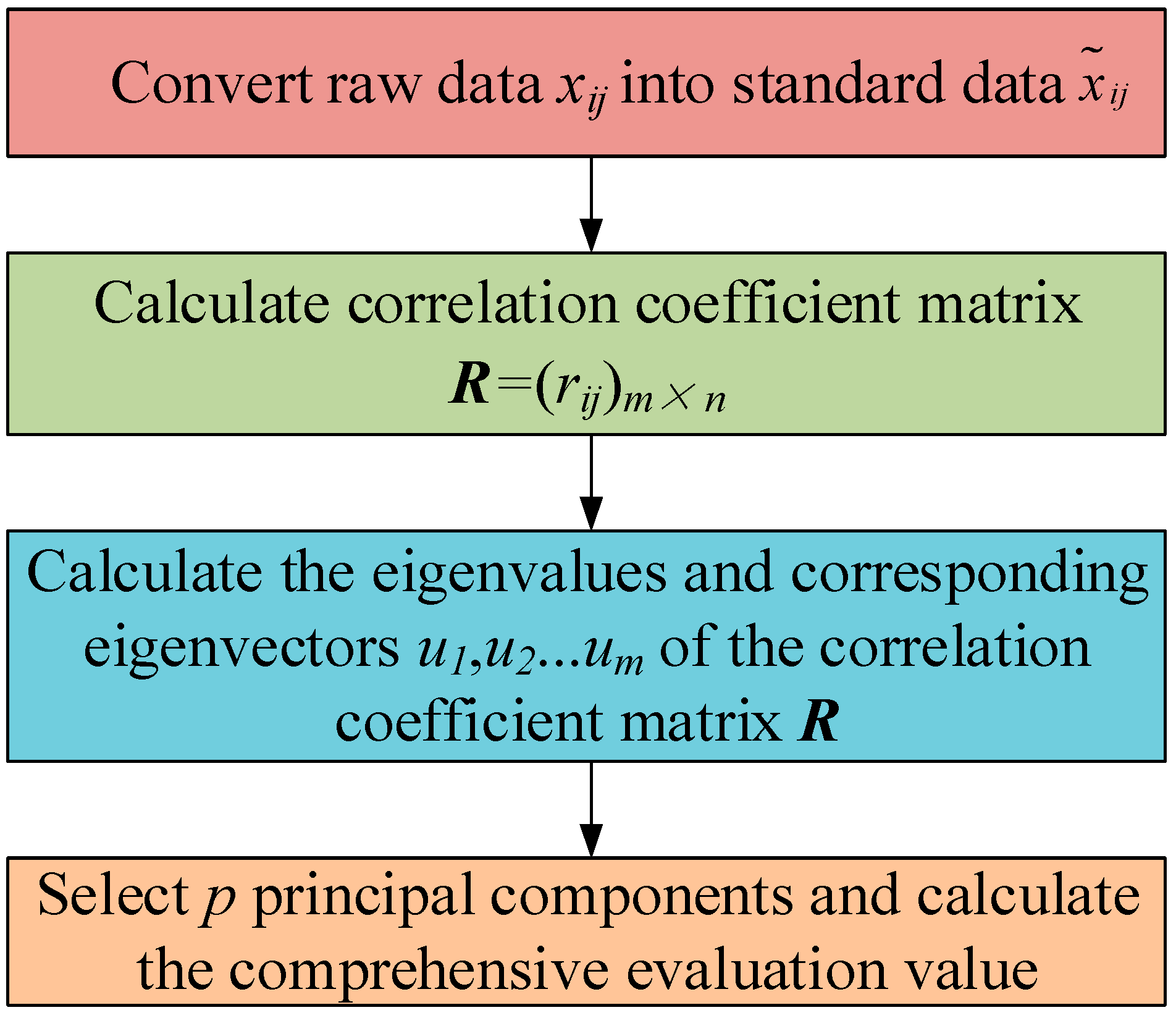
The computation process of the preliminary filtering procedure is shown in Figure 3. The computational flow of the initial screening process is as follows:
Step 1: Standardize the processing of the raw data: by considering that xij denotes the value of the j-th indicator of the i-th evaluation object, xij is converted into a standardized indicator x ¯ i j using the following equations as
x ˜ i j = x i j x ¯ j s j , ( i = 1 , 2 , n ; j = 1 , 2 , m ) ,
x ¯ j = 1 n i = 1 n x i j ,
s j = 1 n 1 i = 1 n x i j x ¯ j 2 , ( j = 1 , 2 , m ) ,
where x ¯ j and sj are the sample mean and standard deviation of the i-th indicator, respectively, and x ˜ i denotes the standardized indicator variable which can be calculated as
x ˜ i = x i x ¯ i s i , ( i = 1 , 2 , m )
Step 2: Calculate the correlation coefficient matrix R = r i j m × n , where r i j is shown in Equation (15) as
r i j = k = 1 n x ˜ k i x ˜ k j n 1 , ( i , j = 1 , 2 , m ) ,
where rii = 1, rij = rji, and rij denote the correlation coefficient between the i-th and j-th indicators.
Step 3: Calculate eigenvalues and eigenvectors: calculate the eigenvalues of the correlation coefficient matrix R and the corresponding eigenvectors u1, u2, …, um, where uj = (u1j, u2j, …, unj)T and m are the new indicator variables that are composed of eigenvectors. The calculation can be performed using Equation (16) as
y 1 = u 11 x ˜ 1 + u 21 x ˜ 2 + + u n 1 x ˜ n , y 2 = u 12 x ˜ 1 + u 22 x ˜ 2 + + u n 2 x ˜ n , y m = u 1 m x ˜ 1 + u 2 m x ˜ 2 + + u n m x ˜ n , ,
where ym is the m-th principal component.
Step 4: In this step, the information contribution rate bj and cumulative contribution rate ap of the eigenvalue motion λj are calculated (j = 1, 2, …, m), as shown in Equations (17) and (18) as
b j = λ j k = 1 m λ k j = 1 , 2 , m ,
a p = k = 1 p λ k k = 1 m λ k .
When ap is close to 1 (ap = 0.85, 0.90, 0.95), then the first p indicator variables y1, y2, …, yp, which are the considered principal components, are selected to analyze the p principal components instead of the original m indicator variables. The comprehensive score is calculated using Equation (19) and evaluated based on the comprehensive score.
Z = j = 1 p b j y j ,

3.2. Re-Flittering of Indicators

Within the information interaction of the ADMS, the evaluation indicators generally change continuously over time. Due to the continuous interaction in the actual operating environment, the information interaction process will continuously evolve, leading to dynamic changes in those related indicators. The data envelopment analysis (DEA) can be used to remove invalid factors and retain key factors. The DEA can comprehensively consider the performance of multiple indicators and transform them into a unified evaluation system, thereby simplifying the evaluation process and improving evaluation efficiency [19]. The most widely used and mature model within the DEA framework is the CCR (Charnes–Cooper–Rhodes)-DEA model. The CCR-DEA model utilizes θk as the efficiency value of the decision-making unit in the model, reflecting self-evaluation. When calculating the results, it is specified that when the efficiency value is equal to 1, it is a valid DMU (Decision-Making Unit). However, when the efficiency value is less than 1, it is a non-valid DMU. By assuming that a number of n DMUs are participating in the evaluation, a DEA model is constructed as shown in Equations (20) and (22) as
x j = ( x j 1 , x j 2 , , x j m ) T ,
y = y j 1 , y j 2 , , y j s T , j = 1 , 2 , n ,
max u T y 0 v T x 0 ,   s . t . u T y j / v T x j 1 v 0 u 0 ,   j = 1 , 2 , n ,
where y j and x j denote the evaluation indicators of decision unit j, u denotes the weight of y j , v denotes the weight of x j , n denotes the number of decision-making units, and x 0 denotes the evaluation indicators of the decision-making unit to be evaluated.
The fractional programming model involved in the above calculations may require a Charnes–Cooper transformation to better utilize the results of linear programming for further analysis and discussion. The Chames–Cooper transformation is a commonly used mathematical transformation method that can be used to transform fractional programming models into equivalent linear programming models, thereby simplifying the problem-solving process and improving solving efficiency, as shown in Equations (23) and (24), i.e.,
t = 1 v T , w = t v , μ = t u ,
max h j 0 = u T y 0 , s . t . μ 0 w T x j μ T y j 0 , j = 1 , 2 , n w T x 0 = 1 w 0 ,
However, for the information interaction process of the ADMS, many factors cannot be represented by clear indicators. Hence, it is necessary to make corresponding improvements to the model. When the input and output cannot be determined, the instruction input value is set to 1. When determining the input and output, the conventional CCR model can be used for calculation. The improved model is calculated as shown in Equation (25), and the risk matrix is shown in Equation (26) as
max h j 0 = μ r y r , s . t . w r = 1   μ r Y 1   μ r 0   w r 0 ,
Y = y 11 y 12 y 1 n y 21 y 22 y 2 n y n 1 y n 2 y n n ,
where wr denotes the input weight size. The matrix value is brought into the above equation to obtain the optimal solution h j 0 * . If h j 0 * > 1, the indicator is invalid and needs to be removed.

4. Evaluating Index Weight by the ANP

To effectively evaluate the information interaction performance of the ADMS, it is necessary to determine a reasonable and feasible evaluation method to accurately obtain the weight values of the required indicators used for evaluation. In practical applications, complex connections and constraints exist between various indicators, so it is necessary to use more objective and comprehensive evaluation methods to ensure the accuracy and reliability of the evaluation results [20].
To address this issue, the ANP, which comprehensively evaluates the information interactivity of the ADMS by considering the correlation and impact degree of indicators at all levels, is employed. The ANP can comprehensively consider the relationships between various indicators, improve the objectivity and accuracy of the evaluation, and provide more scientific and reliable support for the evaluation results.
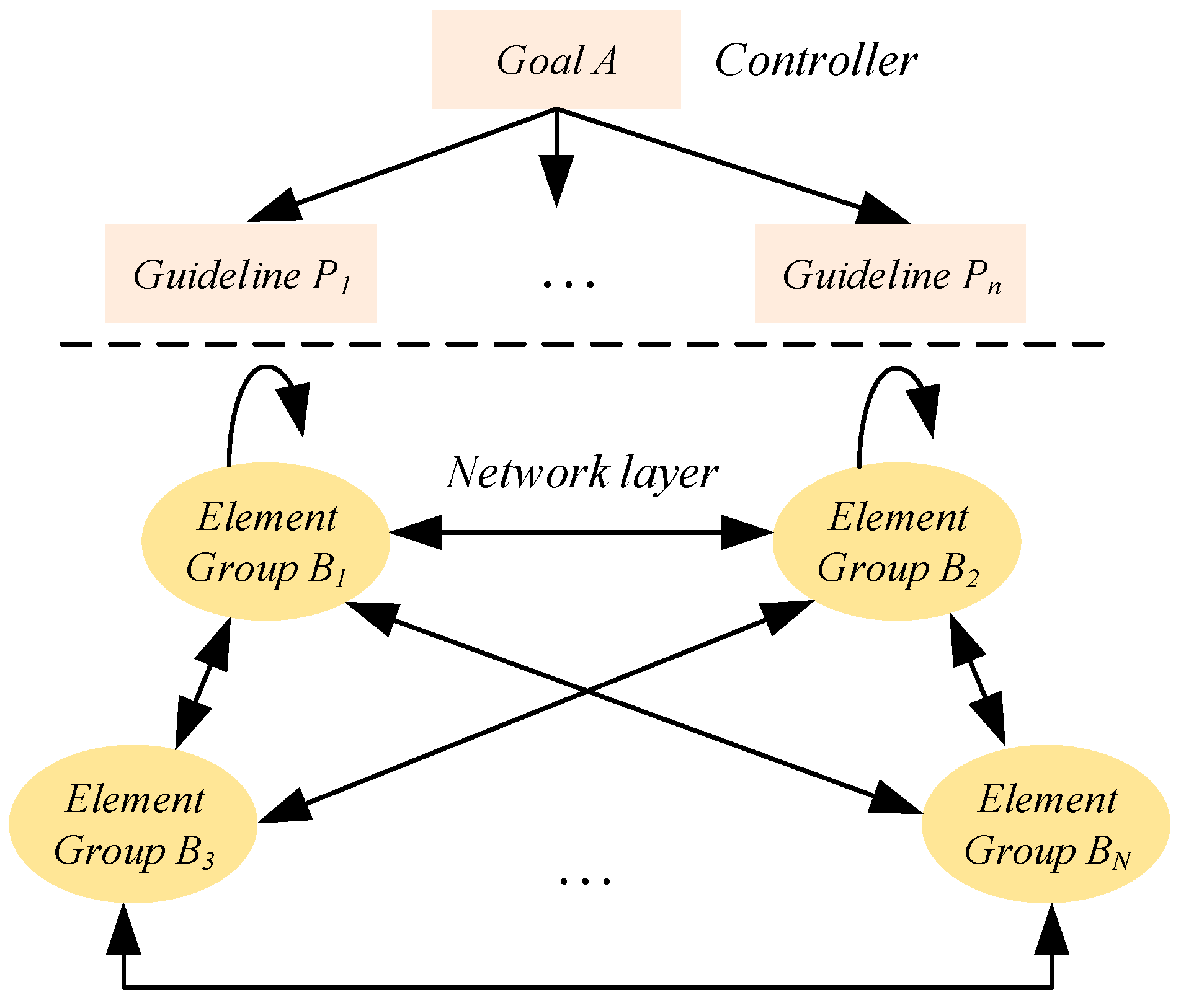
The typical structure of the ANP is shown in Figure 4. Its structure is mainly divided into two levels: (1) the control layer, which is composed of problem objectives and decision criteria; and (2) the network layer, which is composed of all the elements controlled by the control layer which internal elements may affect each other.
The calculation processes of index weighting based on the ANP are as follows:
A-Construction stage
Step 1: Construct a judgment matrix by pairwise comparison.
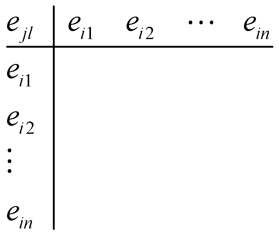
By assuming that the ANP control layer has m criteria, denoted as P1, P2, …, Pm, there are N element groups in the network layer, denoted as B1, …, BN. Among them, element group Bi contains n elements ei1, ei2…, ein (i = 1,2, …, N), and element group Bj contains t elements. By using Ps (s = 1, 2, …, m) as the criterion and element ejl (l = 1, 2, …, t) as the secondary criterion, the indirect dominance of n elements in Bi is compared based on their influence on element ejl (l = 1, 2, …, t), and the corresponding judgement matrix is obtained using the 1–9 scaling method [21]. The corresponding judgement matrix can be realized in Figure 5. Among the elements, if comparing the dominance of factors ei1 and ein yields a score of a, then comparing factor ein with ei1 yields a score of 1/a.
In evaluation methods, common scaling approaches include the three-scale method and the nine-scale method, commonly used to score different indicators or factors. The three-scale method uses three levels or degrees for scoring, usually low, medium, and high. Nevertheless, the nine-scale method uses nine levels or degrees for scoring, which can provide more detailed and accurate evaluation results. Therefore, in actual evaluation, the nine-scale method has higher evaluation accuracy compared to the three-scale method. In this paper, the 1–9 scale method is considered, as shown in Table 1.
Step 2: Construct a meta matrix.
The eigenvectors of the judgment matrix are determined and normalized to obtain the vectors [ w i 1 j l , w i 2 j l , , w i n j l ] T . Then, the sub-block Wij of the hypermatrix is obtained, as shown in Equation (27), i.e.,
W i j = ω i 1 j 1 ω i 1 j 2 ω i 1 j t ω i 2 j 1 ω i 2 j 2 ω i 2 j t ω i n j 1 ω i n j 2 ω i n j t
The column vector of Wij is the sorting vector for the degree of influence of elements ei1, ei2, …, ein in Bi on elements ej1, ej2, …, ejn in Bj. If the elements in Bj are not affected by the elements in Bi, then Wij = 0. The final hypermatrix W is shown in Equation (28), i.e.,
W = W 11 W 12 W 1 N W 21 W 22 W 2 N W N 1 W N 1 W N N
Step 3: Construct a weighted meta matrix.
Using Ps (s = 1, 2, …, m) as the criterion and Bj (=1, 2, …, N) as the sub-criterion, a judgment matrix is constructed using the nine-scale method to obtain the importance weights of each element group for Bj (j = 1, 2, …, N) and then normalized. The sorting vector [a1j, a2j, …, aNj]T is obtained, and the corresponding component vector for element groups unrelated to Bj is zero. The sorting vector corresponding to each element group is determined, and the weighted matrix is obtained, as shown in Equation (29).
A = a 11 a 12 a 1 N a 21 a 22 a 2 N a N 1 a N 1 a N N .
Therefore, the sub-blocks of the weighted hypermatrix W can be calculated using Equation (3) as
W i j = a i j W i j .
where a i j represents the elements of the super matrix, and Wij is the sub-block of the super matrix.
Step 4: Construct the limit hypermatrix.
In this paper, ω ¯ i j denotes the elements in the weighted hypermatrix mentioned above, which reflects the first-order dominance between element i and element j. The advantage of i over j can also be denoted as shown in Equation (31).
ω i j 2 = k = 1 N ω i k ω k j ,
where ω ¯ i j 2 , which is called the secondary advantage degree, is an element of W ¯ 2 , and W ¯ 2 is still column-wise normalized.
According to Equation (32), the j-th column of W ¯ represents the control layer element Ps as a criterion, which is the limit relative sorting vector of each element corresponding to element j in the network layer.
W ¯ = lim x ω ¯ i j t .
B-Calculation stage
Step 5: Calculate the weight values of each indicator.
In the process of using the ANP to determine the weights of various indicators in an indicator system, the involved calculation steps are relatively complex, and it is necessary to consider the interrelationships and impacts between various levels of indicators as well as to perform complex matrix calculations and weight allocation. To simplify this process and improve computational efficiency, LINGO mathematical modeling software tools [21] can be used to solve and calculate the hypermatrix and to obtain the corresponding weights of various levels of indicators. This can not only improve the accuracy and reliability of calculations but also reduce the complexity and workload of calculations as well as improve work efficiency.
Finally, the evaluation value of the information interaction in the ADMS is calculated by the weights and scores by experts, as shown in Equation (33).
E V = 1 n w i p i ,
where w i and p i denote the weight and the score of the i-th indicator, respectively.
The processes of obtaining indicator weights through this method are shown in Figure 6.

5. Simulations and Analysis

The results are collected after selecting actual sample data from the automatic distribution master station and importing the data into the software for principal component analysis. The obtained correlation matrix is partially shown in Table 2, and the total variance explanation is shown in Table 3.
According to Equations (17) to (19), it can be inferred that the first six indicators can be selected as representatives to achieve preliminary screening and degradation of indicator dimensions.
From Table 4, the relationship between the six principal components and various indicators can be seen through the component matrix. The high correlation is noticed between principal component R1 and the indicators A2, B2, and D2, which are the feeder fault-finding time, abnormal frequency, and data cross-region update delay, respectively. Therefore, the principal component of R1 is the transmission speed. The correlation between the principal component R2 and the safe operation rate A4, the packet loss rate C1, and the screen retrieval response time D1 is also high. Therefore, the principal component of R2 is safe operation time. The correlation between principal component R3 and the message integrity rate A5, the forward transmission bandwidth B4, and the transmission error rate C2 is high as well. Therefore, the principal component of R3 is the accurate transmission rate. Also, a high correlation between principal component R4 and the operation ticket qualification rate A3, the abnormal frequency B2, and the remote control output delay D3 is noticed. Therefore, the principal component of R4 is the abnormal monitoring time. Moreover, the correlation between principal component R5 and the alarm frequency A1, the remote control success rate C3, and the data cross-region update delay D2 is clearly high. Therefore, the principal component of R5 is the fault analysis time. The correlation between principal component R6 and the message integrity rate A5, the feeder automation coverage rate B3, and the remote signaling accuracy C4 can be seen as high. Hence, the principal component of R6 is the signal transmission time. Based on the above explanations, those evaluation indicators, including R1, R2, R3, R4, R5, and R6, are preliminarily filtered by the PCA. After the preliminary filtering of those indicators, the number of indicators is reduced to 6, but some redundancies between the indicators remain. To avoid interference, the data envelopment method is used to filter the preliminary data for those 6 indicators, then the invalid indicators are deleted, and finally the weights are assigned to the remaining indicators via the ANP.
In the re-filtering process of the preliminary data, the 6 indicators are marked by the invited experts in the field, and the scoring results are shown in Table 5. Among the six indicators, those with the highest scores, R1, R2, R3, and R4, have the greatest impact on the information interaction. The larger the indicators R1, R2, R3, and R4, the better the operating characteristics of the main station. Therefore, R1, R2, R3, and R4 are considered as input values. However, the fault-finding time R5 and the abnormal frequency R6 have adverse effects on information interaction. The larger the indicators R5 and R6, the worse the operating characteristics of the main station. Therefore, they are considered as output values. If the output result is greater than 1, the expert rating is invalid and needs to be deleted. The scoring results are shown in Table 6.
From Table 6, according to the scores given by experts for each indicator, it can be concluded that scores greater than 1 from Experts 1, 3, and 5 are invalid, while those equal to 1 will be retained, and only the scores from Experts 2 and 4 need to be analyzed. According to the scores from Experts 2 and 4, the calculation results of R2, R5, and R6 are all 0, indicating that these three evaluation indicators have little impact on information interaction and can be removed. After the re-filtering of preliminary data, there are three remaining indicators, namely R1, R3, and R4, with their weights and scores calculated by experts shown in Table 7. Based on Equation (33), the final evaluation value in the section is 92.60, Table 8 indicates that the information exchange of ADMS works best in this situation.
After verifying the evaluation effect of the proposed method in this article, different methods are selected for comparison. The AHP model directly calculates the weights of 16 selected indicators and selects 3 indicators closely related to the performance of the main station [9]. The ANP model directly calculates the weights of 13 selected indicators and selects 4 indicators closely related to the performance of the main station [16]. After the initial screening, the model produces 6 indicators from 25 indicators [20]. After the second screening, the 6 indicators are reduced to 4 indicators that are used as input layer data for the Back-Propagation Neural Network (BPNN). The neuron number of the hidden layer is set as 5, the output indicator is the expected value; therefore, the number of output layers is 1. Table 9 shows that after comparing the evaluation accuracy of different methods, the proposed method has the highest accuracy.

6. Conclusions

The system performance of the ADMS is closely related to the safety, reliability, accuracy, and timeliness indicators of information interaction in the ADMS. This paper has introduced a multiple-indicator filtering-based evaluation method in detail. According to the simulations, the following remarks can be concluded: (1) It has been noted that the safe operation rate, the message integrity rate, the remote control success rate, and the remote signaling accuracy rate can be used to accurately evaluate information interaction. (2) It has been demonstrated that the feeder fault search time, the message integrity rate, and the anomaly frequency have shown similar effects when evaluating the information interaction performance of an ADMS. Overall, this proposed method can be used to evaluate the information interaction performance of an ADMS and can be applied to solve similar tasks in electrical power systems.
Finally, it should be noted that machine learning is a potential tool for evaluating information interaction performance. Therefore, the use of machine learning to further improve the evaluation of the information interaction performance of an ADMS will be addressed in future work. Additionally, abnormal data, and even bad data, might affect the accuracy of our proposed method. Therefore, the problem of abnormal information interaction to assess the sensitivity of the proposed method to sample and guarantee the information interaction evaluation performance of the ADMS needs to be also solved in future work.

Author Contributions

Writing—original draft, R.Z.; writing—review and editing, P.L., J.S. and J.L.; data analysis, K.W. and W.G. All authors have read and agreed to the published version of the manuscript.

Funding

This research was funded by the National Key Research and Development Program: Joint research and development and demonstration of collaborative energy management and operation optimization technology for “Belt and Road” National Urban Smart Energy Network (524608200157).

Data Availability Statement

The data that support the findings of this study are available from the corresponding author upon reasonable request due to privacy, legal and ethical reasons.

Conflicts of Interest

Authors Peng Li, Jinyuan Shi and Kailin Wang were employed by the company NARI Group Co., Ltd. and NARI Technology Nanjing Control Systems Co., Ltd. Authors Ruifeng Zhao, Jiangang Lu and Wenxin Guo were employed by the company Power Dispatching Control Center, Guangdong Power Grid Corporation. The authors declare that the research was conducted in the absence of any commercial or financial relationships that could be construed as a potential conflict of interest.

References

  1. Chen, P.; Tao, S.; Xiao, X.; Wang, X.; Tang, G. An interval model to analyze the voltage level of uncertainty in distribution network. Proc. CSEE 2018, 38, 1035–1044. [Google Scholar]
  2. Lee, P.C.; Zheng, L.L.; Lo, T.P.; Long, D.B. A Risk Management System for Deep Excavation Based on BIM-3DGIS Framework and Optimized Grey Verhulst Model. KSCE J. Civ. Eng. 2020, 24, 715–726. [Google Scholar] [CrossRef]
  3. Fei, S. Overview of application of big data technology in power distribution system. Proc. CSEE 2018, 38, 85–96. [Google Scholar]
  4. Tang, G.; Chen, Q.; Jin, X. Research on Interaction and Application Technology of Distribution Network Automation Master Station. Microcomput. Appl. 2023, 39, 49–52. [Google Scholar]
  5. Tang, H.; Tang, Z.; Qiu, G. Design of an Intelligent Distribution Network Visualization Platform Based on Information Interaction. Inf. Technol. 2023, 175–179+184. [Google Scholar]
  6. Wang, H. The Design and Implementation of Power Supply Company Distribution Master Automation Data Monitoring System for Rongcheng City. Ph.D. Thesis, Shandong University, Jinan, China, 2016. [Google Scholar]
  7. Zhang, Y.; Zhu, J.; Yan, W.; Xian, Y.; Qi, Y.; Wang, X. Application of AI language function in distribution automation main station. Power Equip. Manag. 2021, 23–24+44. [Google Scholar]
  8. Zhang, P.; Ding, Y.; Ge, L.; Xian, Y.; Qi, Y.; Wang, X. Functional design and information interaction technology for new distribution automation master stations. Power Capacit. React. Power Compens. 2020, 41, 126–134+140. [Google Scholar]
  9. Jia, L.; Gao, Y.; Ge, L.; Chen, B.; Wang, Y.; Zhang, P. AHP fuzzy comprehensive evaluation method for information interaction of new generation distribution main stations. J. Power Syst. Autom. 2020, 32, 1–6. [Google Scholar]
  10. Heydt, G.T. The next generation of power distribution systems. IEEE Trans. Smart Grid 2010, 1, 225–235. [Google Scholar] [CrossRef]
  11. Pirouzi, S.; Zaghian, M.; Aghaei, J.; Chabok, H.; Abbasi, M.; Norouzi, M.; Shafie-khah, M.; Catalão, J.P. Hybrid planning of distributed generation and distribution automation to improve reliability and operation indices. Int. J. Electr. Power Energy Syst. 2022, 135, 107540. [Google Scholar] [CrossRef]
  12. Kazemi, S.; Fotuhi-Firuzabad, M.; Billinton, R. Reliability assessment of an automated distribution system. IET Gener. Transm. Distrib. 2007, 1, 223–233. [Google Scholar] [CrossRef]
  13. Chen, Y.; Wang, M.; Lin, T.; Wang, Z.; Lv, L.; Wang, G. Research on Big Data Processing and Testing Technology for Large Distribution Automation Main Stations. Power Supply Consum. 2019, 36, 30–35. [Google Scholar]
  14. Tallon-Ballesteros, A.J. A Master Station and Terminal Data Exchange Method Based on Symmetric and Asymmetric Algorithms. In Proceedings of the 11th International Conference on Electronics, Communications and Networks, Virtual Event, 18–21 November 2021. [Google Scholar]
  15. Yue, D. Deep Integration of Information Interaction in Distribution Automation Systems. Rural. Electrif. 2018, 5, 41–43. [Google Scholar]
  16. Ding, Y.; Ge, L.; Zhang, P.; Liu, C.; Wang, Y.; Wu, L. ANP evaluation method for information security of new generation distribution automation main stations. J. Power Syst. Autom. 2019, 31, 83–88. [Google Scholar]
  17. Ji, Y. Research on Optimal Scheduling Method For Microgrid Considering Source Load Uncertainty. Ph.D. Thesis, Xi’an University of Technology, Xi’an, China, 2024. [Google Scholar]
  18. Sun, W.; Wang, W.; Zhang, Z.; Wu, H.; Zhu, Y. PV Power Range Prediction Based on Principal Component Analysis and Long Short-term Memory Neural Network. Jilin Electr. Power 2024, 52, 1–5. [Google Scholar]
  19. Yan, M. Application of secondary security in main station system of distribution automation. Electron. Technol. Softw. Eng. 2017, 133. [Google Scholar]
  20. Gao, H.; Huang, X. Risk assessment of deep foundation pit construction based on improved AHP-BP. J. Eng. Manag. 2023, 37, 147–152. [Google Scholar]
  21. Saaty, T.L. Principles and Applications of Network Analytic Hierarchy Process; Beijing Institute of Technology Press: Beijing, China, 2015. [Google Scholar]
Figure 1. The typical architecture of the ADMS.
Energies 17 03552 g001
Figure 2. Comprehensive evaluation indicator system for information interaction in ADMS.
Energies 17 03552 g002
Figure 3. The computation process of the preliminary filtering procedure.
Energies 17 03552 g003
Figure 4. Typical structure of ANP.
Energies 17 03552 g004
Figure 5. The typical structure of the corresponding judgement matrix.
Energies 17 03552 g005
Figure 6. Flowchart of indicator weighting based on ANP.
Energies 17 03552 g006
Table 1. Scoring Scale.
Scoring ScoreImportance
1Two elements have the same importance compared to each other.
3Compared to two elements, one element is slightly more important than the other element.
5Compared to two elements, one element is significantly more important than the other.
7Compared to two elements, one element is more strongly important than the other element.
9Compared to two elements, one element is extremely important compared to the other element.
2,4,6,8The median of the above adjacent judgements.
Table 2. Correlation matrix.
Z1Z2Z3Z4Z5
Z11.000−0.1020.603−0.2960.418
Z2−0.1021.000−0.197−0.457−0.563
Z30.603−0.1971.000−0.2380.699
Z4−0.296−0.457−0.2381.0000.153
Z50.418−0.5630.6990.1531.000
Table 3. Total variance explanation.
ComponentInitial Eigenvalue
TotalVariance PercentageCumulative/%
18.46734.27836.792
25.26725.58857.458
34.86715.87365.275
43.67110.84579.823
53.4726.36290.194
61.2823.17597.168
7
163.654 × 10−102.763 × 10−9100.00
Table 4. Component matrix.
R1R2R3R4R5R6
A1−0.1760.245−0.5560.1200.4530.151
A20.567−0.5560.245−0.734−0.556−0.135
A30.2960.348−0.2560.4570.3480.088
A4−0.7340.4530.057−0.3670.028−0.246
A5−0.4570.3360.477−0.4250.3360.478
B10.342−0.7340.3460.164−0.734−0.526
B20.7990.348−0.4550.945−0.4570.245
B3−0.2470.453−0.668−0.4600.3420.686
B4−0.8450.3360.568−0.1070.194−0.455
C10.4570.499−0.5660.346−0.247−0.405
C2−0.257−0.2570.426−0.4550.194−0.868
C30.3560.3560.256−0.6680.9340.378
C40.2870.287−0.2090.426−0.1890.767
D1−0.5020.8140.1680.309−0.6470.364
D20.934−0.5020.109−0.5660.739−0.386
D30.4680.468−0.4580.7280.4570.296
Table 5. Scores After Initial Filtering.
Expert No.R1R2R3R4R5R6
1#156473
2#245538
3#377154
4#184225
5#368143
Table 6. Calculation Expert Scoring Results.
Expert No.minR1R2R3R4R5R6
1#1.100.120.100.240.370.000.50
2#1.000.160.000.330.170.000.00
3#1.230.000.120.000.000.140.36
4#1.000.000.000.000.000.000.00
5#1.450.130.000.130.150.250.27
Table 7. Indicator Weights For Information Interaction Systems.
IndicatorWeightScore by Experts
R10.32990.174
R30.28493.058
R40.38794.326
Table 8. Hierarchical Evaluation Degree.
Evaluation DegreeValueScore by Experts
Best90–100Best
Well80–89Well
Satisfactory70–79Satisfactory
Normal60–69Normal
Worse<59Worse
Table 9. Different method comparisons.
MethodAccuracy
AHP [9]86.23%
ANP [16]89.37%
AHP-BP [20]93.76%
Proposed method of our paper98.41%
Disclaimer/Publisher’s Note: The statements, opinions and data contained in all publications are solely those of the individual author(s) and contributor(s) and not of MDPI and/or the editor(s). MDPI and/or the editor(s) disclaim responsibility for any injury to people or property resulting from any ideas, methods, instructions or products referred to in the content.