Article

Impact of Stationarizing Solar Inputs on Very-Short-Term Spatio-Temporal Global Horizontal Irradiance (GHI) Forecasting

by
Rodrigo Amaro e Silva
1,2,
Llinet Benavides Cesar
3,*,
Miguel Ángel Manso Callejo
3 and
Calimanut-Ionut Cira
3
1
Centre Observation, Impacts, Energy, MINES ParisTech, PSL Research University, 06904 Sophia Antipolis, France
2
Instituto Dom Luiz, Faculdade de Ciências, Universidade de Lisboa, Campo Grande, 1749-016 Lisboa, Portugal
3
Departamento de Ingeniería Topográfica y Cartográfica, Escuela Técnica Superior de Ingenieros en Topografía, Geodesia y Cartografía, Universidad Politécnica de Madrid, C/Mercator 2, 28031 Madrid, Spain
*
Author to whom correspondence should be addressed.
Energies 2024, 17(14), 3527; https://doi.org/10.3390/en17143527
Submission received: 8 May 2024 / Revised: 23 June 2024 / Accepted: 15 July 2024 / Published: 18 July 2024
(This article belongs to the Special Issue Advances in Solar Systems and Energy Efficiency: 2nd Edition)

Abstract

:
In solar forecasting, it is common practice for solar data (be it irradiance or photovoltaic power) to be converted into a stationary index (e.g., clear-sky or clearness index) before being used as inputs for solar-forecasting models. However, its actual impact is rarely quantified. Thus, this paper aims to study the impact of including this processing step in the modeling workflow within the scope of very-short-term spatio-temporal forecasting. Several forecasting models are considered, and the observed impact is shown to be model-dependent. Persistence does not benefit from this for such short timescales; however, the statistical models achieve an additional 0.5 to 2.5 percentual points (PPs) in terms of the forecasting skill. Machine-learning (ML) models achieve 0.9 to 1.9 more PPs compared to a linear regression, indicating that stationarization reveals non-linear patterns in the data. The exception is Random Forest, which underperforms in comparison with the other models. Lastly, the inclusion of solar elevation and azimuth angles as inputs is tested since these are easy to compute and can inform the model on time-dependent patterns. Only the cases where the input is not made stationary, or the underperforming Random Forest model, seem to benefit from this. This indicates that the apparent Sun position data can compensate for the lack of stationarization in the solar inputs and can help the models to differentiate the daily and seasonal variability from the shorter-term, weather-driven variability.

1. Introduction

In solar forecasting, an increasingly important area of study for the cost-effective integration of solar energy [1], there exists a well-established practice of stationarizing solar time series when building forecasting models: to remove the intrinsic and predictable daily and annual seasonality from raw solar time series, allowing models to discern weather-driven variability more effectively [2,3]. This was shown to be more effective than generic input normalization approaches when training machine-learning models for solar irradiance forecasting [4]. To achieve this, global horizontal irradiance (GHI), for example, is converted into either the clearness ( K t ) or clear-sky ( K c ) index (c.f. Section 2). Furthermore, there are other applications that exploit these same indices: global irradiance decomposition [5,6], temporal downscaling [7,8], clear-sky identification [9,10], synthetic data generation [11], stochastic variability analysis [12], or even PV performance analysis [13].
The persistence model (a baseline forecasting method assuming that the future, at a given time horizon, mirrors a past observation) serves as a clear illustration of the necessity of stationarization. Without this preprocessing, unless the forecast horizon aligns precisely with multiples of 24 h, this approach will inevitably introduce a delay in capturing the predictable seasonality of the targeted solar variable (an example of this is presented in Figure 1). If, instead, a stationarized version of said variable is persisted and then reconverted to its original form, an approach commonly referred to as smart persistence, the model can account for variations in the apparent Sun position and is not penalized due to the lag in the daily profile. Interestingly, there are also works proposing the persistence of the variation through time of such stationary variables to account for changes in cloud thickness [14].
Although commonly employed in the literature, both for baseline and state-of-the-art statistical approaches, the impact of this preprocessing step is seldom quantified.
Lorenzo et al. evaluate, among other things, various persistence approaches, one of which is the clear-sky index smart persistence [15]. Considering a location in Tucson, Arizona, the results show that, up to 10 min ahead, the simple and smart persistence yield similar results, after which the performance of smart persistence degrades slower than its simple version (with a difference of 7.5% in the RMSE for 30 min ahead).
Lauret et al. [16] test the impact of using either the GHI, K t , or K c as input for three distinct autoregressive models, for six locations across the globe with different climates, covering a horizon between 1 and 6 h: persistence, linear regression, and a non-linear Artificial Neural Network (ANN). The results suggest that the K c benefits autoregressive forecasting models. Furthermore, the authors highlight how the ANN is more capable of extracting useful information from the K t , outperforming the simpler approaches, even when these consider the K c . Additionally, the authors point out that for locations characterized by high variability, both indices lead to similar performance levels.
When using the K c as input, the choice of the clear-sky model also comes into play. Yang [17], Eschenbach et al. [18], and Mendonça de Paiva et al. [19] evaluate this aspect and conclude that the mentioned choice has minimal impact on the forecast performance. Within the scope of a baseline method that combines climatology and persistence, Yang considers three solutions: (1) Ineichen-Perez [20], (2) McClear [21], (3) and REST2 [22]. In contrast, for an ANN-based spatio-temporal approach, Eschenbach et al. test two models: (1) McClear [21] and (2) Haurwitz [23].
To the best of the authors’ knowledge, there has been no previous comprehensive assessment of the impact of solar input stationarization conducted specifically for spatio-temporal solar-forecasting approaches, a domain where spatially distributed solar time series have proved to enhance forecasting accuracy by capturing cloud advection patterns [24]. The work by Eschenbach et al. [18] stands as the only exception, albeit focusing solely on the choice of the clear-sky model.
A recent review shows that a considerable share of spatio-temporal solar-forecasting publications address sub-hourly timescales [25]. Analyzing this body of literature shows that 77% of the works exploiting spatially distributed in situ data actually consider a temporal resolution up to 10 min. This is possibly due to high-resolution data allowing for a more detailed observation of cloud-driven variability and the availability of one widely recognized public data set from the National Renewable Energy Laboratory (NREL) for which the local climate has been described in a detailed manner.
Thus, this work aims to open the discussion on the impact of stationary solar inputs for spatio-temporal solar forecasting by first covering the second to minute timescales, hopefully paving the way for future studies addressing a broader range of spatio-temporal scales. This is accomplished by testing five different forecasting models: a baseline (persistence), one linear model (linear autoregressive model using exogenous inputs), and three non-linear tree-based models (Random Forest and two versions of Gradient Boosting). The choice of tree methods was based on their suitability for solar-forecasting tasks [26]. Furthermore, the inclusion of the Sun’s apparent position was also investigated, since this information may compensate for the lack of, or enhance the use of, stationary solar irradiance inputs.
This study aims to achieve the following two objectives:
  • Quantify the impact of stationarizing solar irradiance time series on forecasting performance within the scope of very-short-term spatio-temporal GHI forecasting. While this preprocessing step is commonly implemented in the literature, its actual effect on forecasting performance remains largely unexplored.
  • Evaluate how the inclusion of variables describing the apparent Sun position interacts with both raw and stationarized irradiance inputs in such forecasting models, namely, in terms of the forecasting accuracy.
The present paper is structured as follows. Section 2 describes the data and the models studied and presents the methodology applied to perform meaningful comparisons, Section 3 discusses the obtained results, while Section 4 presents the conclusions.

2. Methodology

2.1. Data

2.1.1. Global Horizontal Irradiance

The dataset used, the Oahu Solar Measurement Grid from Hawaii [27], contains GHI measurements with 1 s resolution from 17 sensors spread out over a 1 km2 area (as illustrated in Figure 2) over 19 months (March 2010 to October 2011). The data were resampled to 10 s to avoid introducing any undesired noise, as suggested by Yang et al. [28]. The dataset is well established in the specialized literature and has been used in several studies [11,29,30,31,32,33,34,35]. According to Hinkelman [36], this location is characterized by frequent broken clouds (cumulus) and prevailing trade winds from the northeast, which drive cloud advection.

2.1.2. Sun Elevation and Azimuth

The apparent Sun position, described by the elevation and azimuth angles, was calculated using the “Solar Geometry 2” (SG2) Python package [37] (available on GitHub [38]). This package was also used to calculate the top-of-the-atmosphere solar irradiance discussed in the next section.
The elevation angle was used to filter the data considered in the model training and validation (see Section 2.4), and both the elevation and azimuth were used as supplementary input variables when training the statistical models (see Section 3.5).

2.1.3. Clearness Index

The clearness index ( K t ) is calculated as the ratio between the GHI and the irradiance at the top of the atmosphere (defined in Equation (1)), and it quantifies the attenuation resulting from the airmass, aerosols, water vapor, and clouds.
K t = G H I I 0
In Equation (1), I 0 represents the top-of-the-atmosphere irradiance on the horizontal surface and has been calculated using SG2, which was described before. Since all the pyranometers are installed in a small spatial area (with variations in space always below 0.3 W.m−2), a single calculation for the average position is considered.

2.1.4. Clear-Sky Index

The clear-sky index ( K c ), instead, focuses on cloud-driven attenuation by replacing I 0 with the expected clear-sky irradiance (as presented in Equation (2)).
K c = G H I I c l e a r
In Equation (2), I c l e a r represents the global horizontal irradiance in clear-sky conditions, calculated by the McClear model [21,39] and retrieved using the pvlib application programming interface (API) [40] for this Copernicus Atmospheric Monitoring Services (CAMS) product [41]. Just as for the I 0 , a single request is performed for the average position and all the locations consider the same I c l e a r .

2.2. Implemented Forecasting Methods

2.2.1. Persistence and Smart Persistence Models

Persistence is a naïve forecasting model, where the forecast is assumed to be a past observation of the target value (Equation (3)), in this case of the GHI.
Y t + h = Y t
However, persisting a non-stationary variable such as the GHI disregards the inherent daily cycle of solar irradiance, except for horizons of 24 h multiples. This introduces a source of error into the forecast. To mitigate this, the smart persistence approach instead considers lagged values of a stationarized version of the GHI, such as K t or K c . Subsequently, the forecast is converted back into the GHI by multiplying it by the respective I 0 or I c l e a r , which can be known (or predicted) beforehand.
Because of their simplicity in terms of implementation and minimal data requirements, persistence models are often used as a baseline for benchmarking forecasting models, such as to calculate the Forecast Skill metric (consult Section 2.4).

2.2.2. Multivariate Linear Regression

The multivariate linear regression (described in Equation (4)), also known as a linear auto-regressive model using exogenous (ARX) inputs, is a linear regression (LR) approach that has already been investigated in spatio-temporal works [3,42,43].
Y t = l a l Y ( t l ) + q l a q , l Y q ( t l ) + b
In Equation (4), Y ( t l ) and Y q ( t l ) denote past observations of the target variable Y , with lag l for the location of interest, and its q neighbours; a l and a q , l denote the regression coefficients of the LR model; and b is the model constant term.
It is also interesting to note that LASSO and stepwise variations have been used by Yang et al. [28] and Gagne et al. [44] to avoid overfitting and maximize the forecasting accuracy in the presence of a large amount of input variables.

2.2.3. Tree-Based Models

Here, the Random Forest (RF) and Gradient Boosting (GB) models are tested, since these represent bagging and boosting tree-based approaches, respectively, both exploiting regression trees.
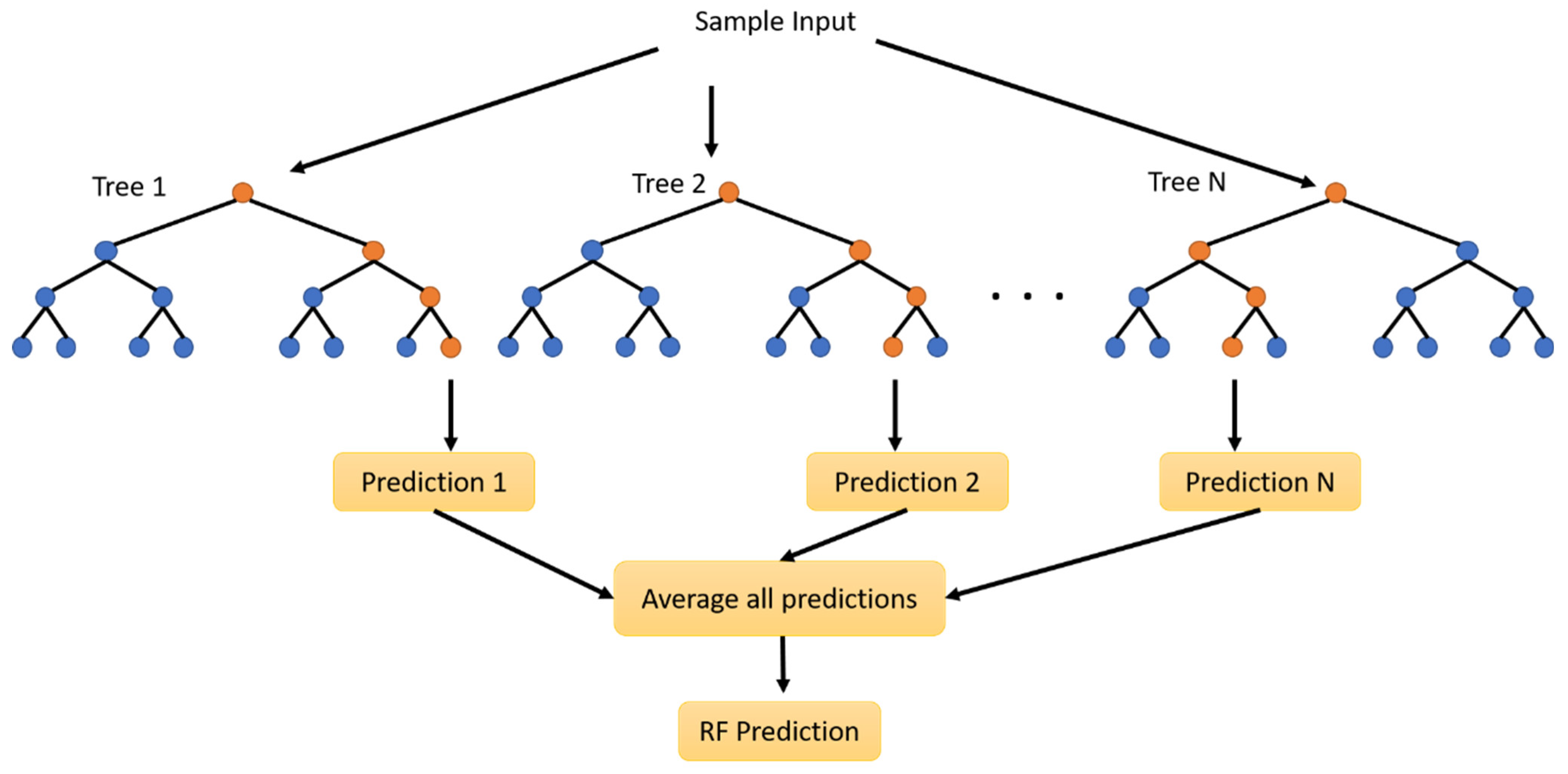
RF [45,46] (described in Figure 3) is a bagging approach, combining multiple regression trees in parallel. A regression tree is a model that divides the predictor space into distinct, non-overlapping regions defined by a set of recursive binary rules (e.g., when a given predictor is either below or is equal or larger than a given threshold), and for each region, the same output is obtained, based on the average of the training samples that fit there.
This results in a tree structure that comprises a set of nodes (binary rules), branches (the paths to the following nodes depending on the result of each binary rule), and leaves (the set of possible outputs that the model arrives at after running each full sequence of rules). To ensure optimal performance, avoid overfitting and achieve low bias, each tree is trained with a different random subset of the training data, and in turn, each split in each tree only considers a random subset of predictors (ensuring diversity across trees).
Gradient Boosting, on the other hand, consists of a set of sequential trees, where each tree is grown using information from the previously grown trees. Each tree, usually shallow to avoid overfitting, aims to predict the residuals of the previous tree, which is then combined with the previous trees to produce a more accurate output with smaller residuals.
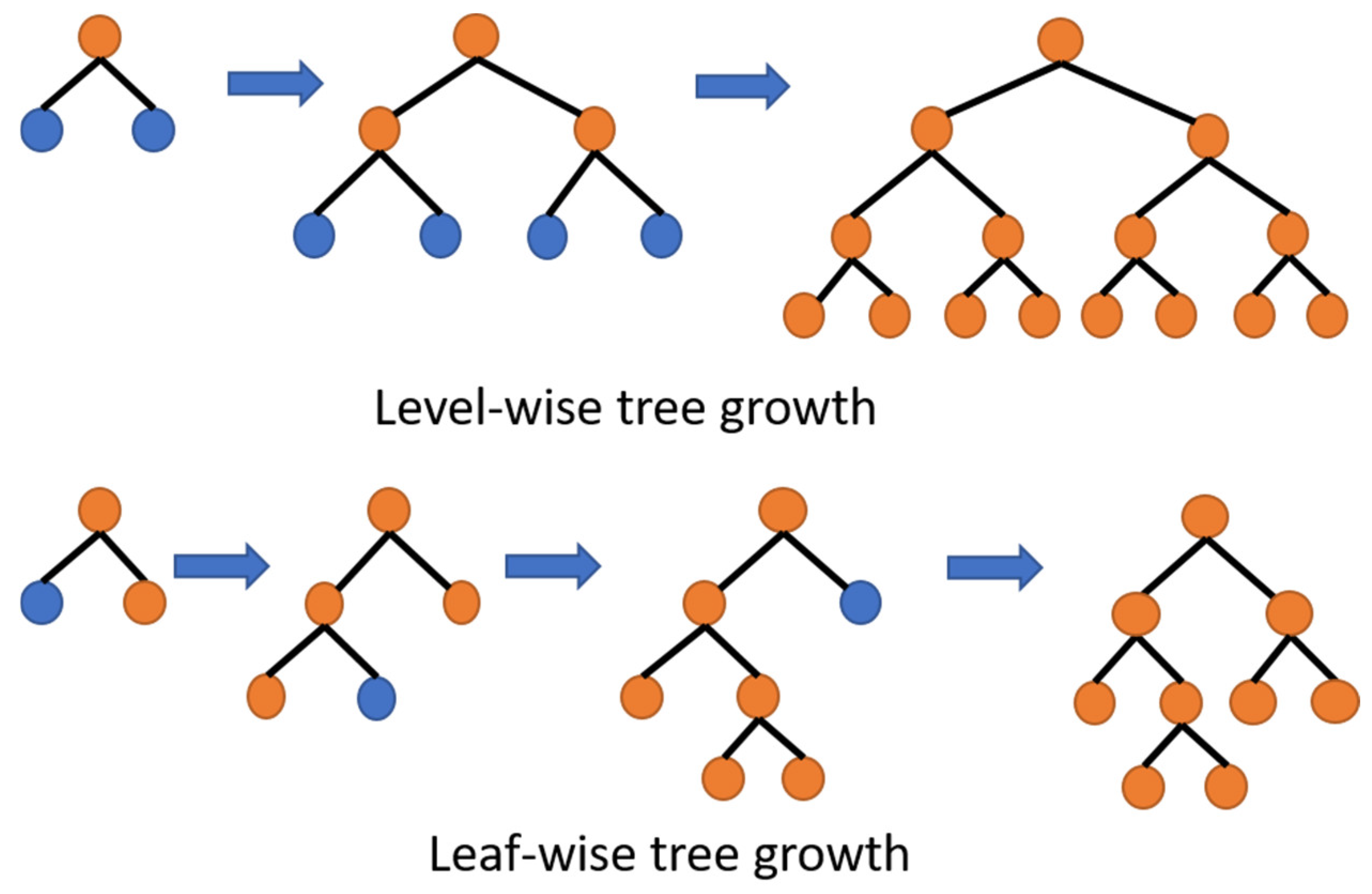
Here, Gradient Boosting is tested using two different implementations: XGBoost (eXtreme Gradient Boosting) [47] and LightGBM [48] (Light Gradient-Boosting Machine). For the first case, the model parameter optimization is driven by the gradient descent, and the trees are grown level-wise (i.e., when adding a level to a tree, all the previous nodes must be followed by a split, as shown in Figure 4). The second case relies on three variations in the training framework to achieve a lighter implementation from which considerable savings in the computational demand are expected at the expense of a comparatively smaller loss of accuracy. These variations are notably the use of Gradient-Based One-Side Sampling and Exclusive Feature Bundling, and growing trees leaf-wise (Figure 4), which focuses in each iteration on the leaf with the highest residuals.
All the models were implemented in Python 3.9, using the sci-kit learn library for training RF models [49], and XGboost [50] and LightGBM [51] for both versions of gradient boosting here considered.

2.3. Inputs Considered

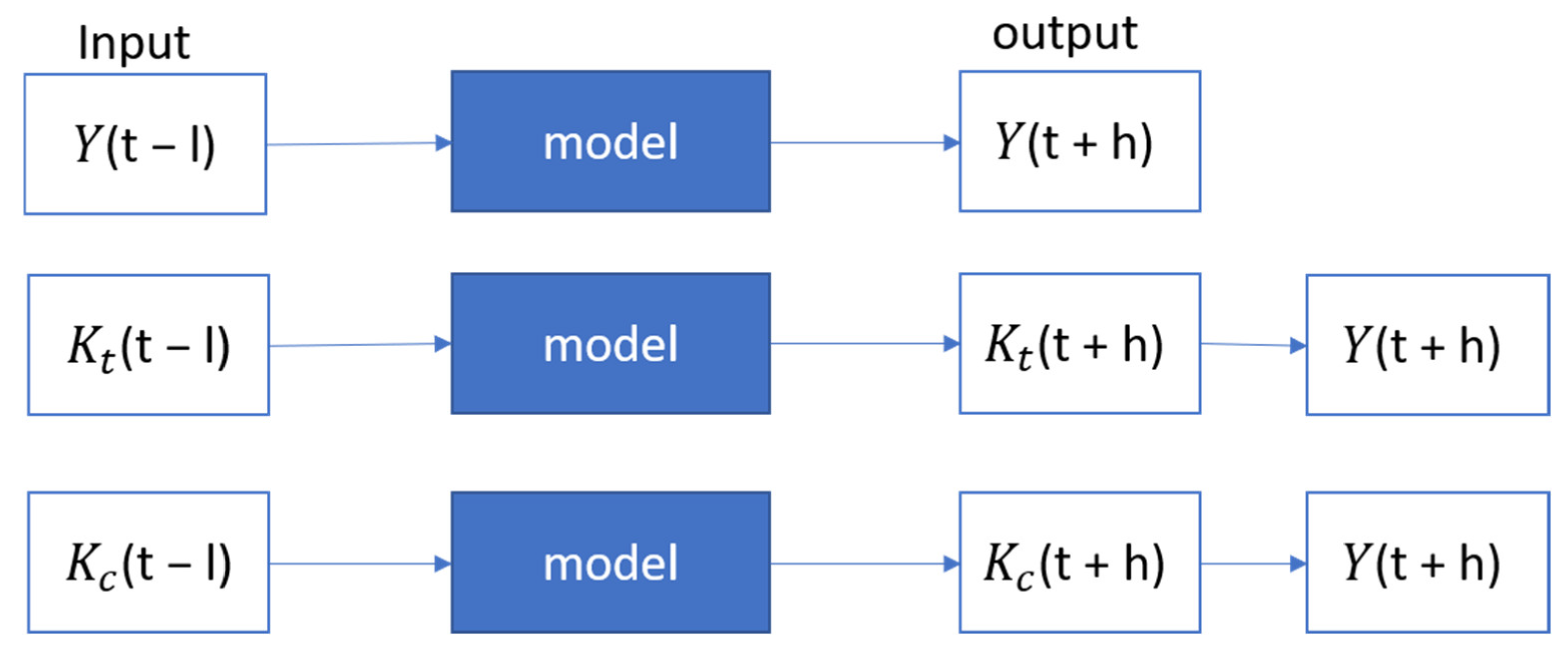
In this work, the persistence approaches consider the latest data to forecast 10 s or 5 min ahead from and for each site independently. The remaining approaches consider the three most recent data points (i.e., from 10 to 30 s before the forecast target time) from all the sites at once to forecast each site independently. It is important to note that, independently of the model, when either Kt or Kc is considered as the input (and, as a result, the output), an additional step is needed to obtain the GHI—multiplying with the respective top-of-the-atmosphere or clear-sky irradiance—as described in Figure 5.
As an additional experiment, non-persistence models are retrained by also considering the apparent position of the Sun (solar elevation and azimuth angles) since this information is related to the seasonality that describes the GHI.

2.4. Hyperparameter Search

Tree-based methods, similar to other machine-learning (ML) approaches, have hyperparameters that need to be defined before the model training. Here, most of the hyperparameters of each model type assume their default values, except for two that are commonly optimized in the literature [52,53,54]. Table 1 lists and briefly describes the parameters and the values tested (also based on [52,53,54]).
Here, the hyperparameter optimization is performed using a grid search approach, testing all the possible parameter combinations. A two-fold cross-validation tailored for time series is applied, which ensures that the training period always precedes the one for validation (i.e., temporal consistency): in the first fold, the last 40% of the training data are used for validation, whereas for the second fold, only the last 20% are considered.
Based on this, the best-performing configuration is retained, and the model is retrained using both training and validation data. The final model is then effectively evaluated using an independent test set. In practice, the model training and validation are carried out using the first 364 days of the dataset to cover all the seasons; the remaining 224 days are then used for testing.

2.5. Performance Metrics

The forecasting performance is evaluated using the forecast skill (FS) based on the root mean squared error (RMSE) [55,56]. The RMSE (defined in Equation (5)) is one of the most common metrics used in forecasting [57], and it focuses on point-by-point deviations, giving more weight to high-magnitude errors (related to changes in cloud cover) due to its squared term.
R M S E = 1 n i = 1 n ( y i y i ^ ) 2
Then, the FS (defined in Equation (6)) compares how well a given model performs compared to a baseline, usually a persistence-based approach (discussed in the next section), allowing for a more robust comparison of performance across different forecast horizons and sites. An FS of zero or lower indicates that the models perform as well as or worse than the baseline, whereas a model outperforming the baseline achieves a positive FS (with a perfect forecast, FS = 1).
F S = 1 R M S E m o d e l R M S E p e r s i s t e n c e
Additionally, complementary metrics such as the mean absolute error (MAE) and the coefficient of determination are presented in Appendix A, Appendix B, Appendix C, Appendix D, Appendix E and Appendix F. These annexes provide additional perspectives regarding the model performance: disregarding the squared term in the RMSE, assigning equal weight to all situations; quantifying the proportion of variance captured by the forecasting model; or focusing on systematic errors.
As low solar incidence angles tend to affect the quality of the measurements, only predictions for solar elevation angles above 5° are considered in the model training and assessment.

3. Results and Discussion

3.1. Evaluation of Baseline Persistence Approaches

As initially discussed in Section 1, persistence approaches commonly serve as baseline benchmarks for evaluating forecasting models. Therefore, comparing the RMSE of the three persistence implementations implemented in this work can be viewed as an initial assessment of the impact of using stationarized inputs in such approaches. Furthermore, understanding their performance can aid in selecting the most suitable (best-performing) one as a reference for calculating the FS.
Based on a subsequent discussion outlined in the following section, this work focuses on two forecast horizons, namely, 30 s and 5 min ahead. Figure 6 shows an expected increase in the RMSE for the longer horizon. However, it also shows that stationarizing the GHI for such short timescales within the scope of a smart persistence model has a negligible effect. The variation is smaller than 0.1% of the mean, which is aligned with the findings reported in [15]. This can be attributed to the subtle lag introduced by this short horizon in the daily profile of the persistence forecast, leading to small deviations that will have minimal impact in the RMSE, given its emphasis on high-magnitude deviations.
Thus, the K t -based smart persistence was selected as the reference baseline for calculating the FS. Despite the minimal impact of this choice, it considers the daily cycle of the GHI and has an easier implementation when compared to the use of its K c counterpart.

3.2. Recapping Spatio-Temporal Patterns Present in the Data

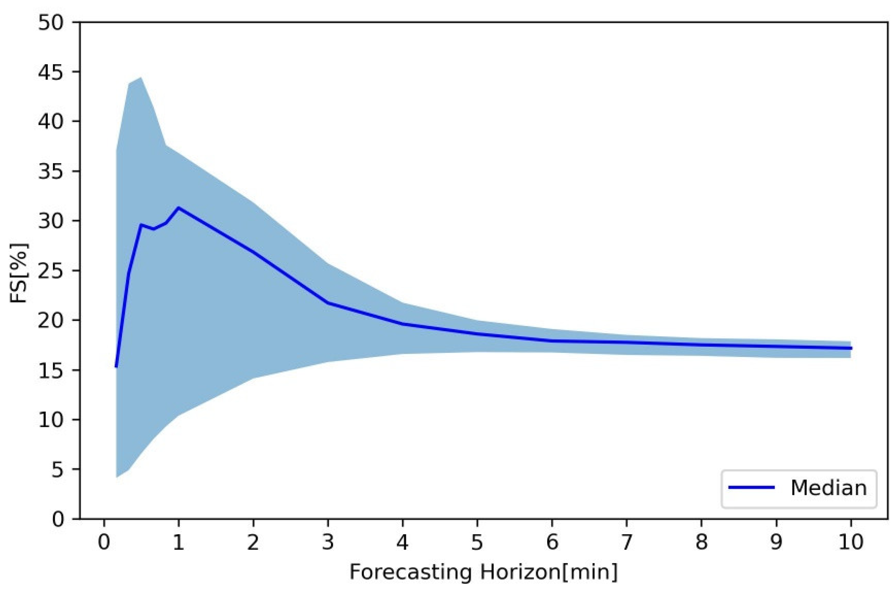
As described by Hinkelman [36], Oahu is characterized by prevailing northeasterly winds that drive the advection of local cumulus clouds. Previous forecasting works have shown how the local wind patterns introduce strong spatio-temporal patterns in the Oahu network solar irradiance dataset [28,58] and how these depend on the timescale under consideration. To revisit the findings from [58], an LR model is trained for each individual station, covering forecast horizons ranging from 10 s to 10 min. Analyzing the fluctuation in the forecast skill across the different horizons, as depicted in Figure 7, reveals two distinct regimes. For shorter horizons, arguably up to 3–4 min ahead, higher FS values can be achieved, reaching up to 45%. However, it is worth noting that there is considerable variability in the performance across stations, with the minimum values reaching 5–10%. On the other hand, for longer horizons, the achieved FS is more moderate, around 15%, yet it exhibits greater consistency across stations.
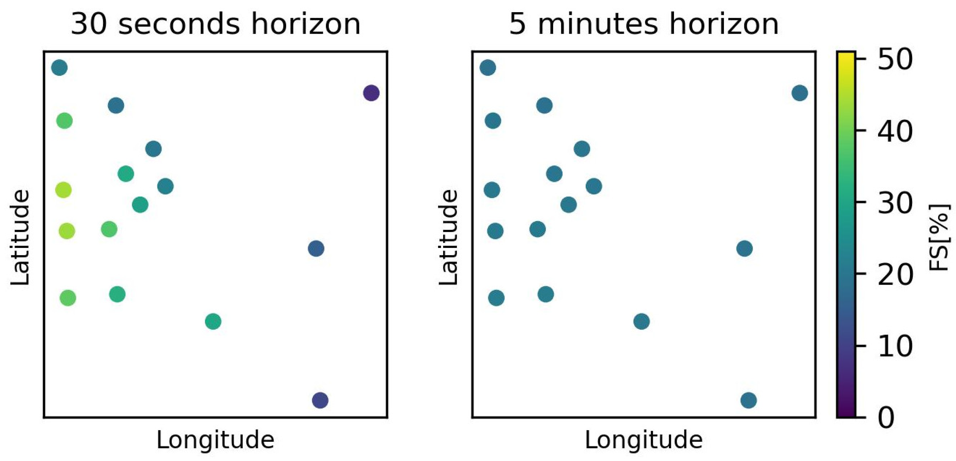
As illustrated in Figure 8, when the FS values are plotted for the 30 s horizon (where maximum skill is achieved), it is possible to observe how these results are a consequence of the sensor network layout and local wind patterns: sensors with nearby neighbors in the northeast direction (i.e., upwind) perform well, in contrast with the other stations (Figure 8, left). For a 5-min horizon, it can be observed that all the sites achieve a similar FS and perform better than the worst sites for the shorter horizon (Figure 8, right). Amaro e Silva and Centeno Brito [58] argue that since this temporal scale surpasses the limited spatial coverage of the network sensor, the model can no longer detect advection patterns. However, the degradation of the persistence baseline, as the autocorrelation factor decreases with the horizon, still allows room for spatially distributed solar information to contribute to a better forecast, as is explained next.
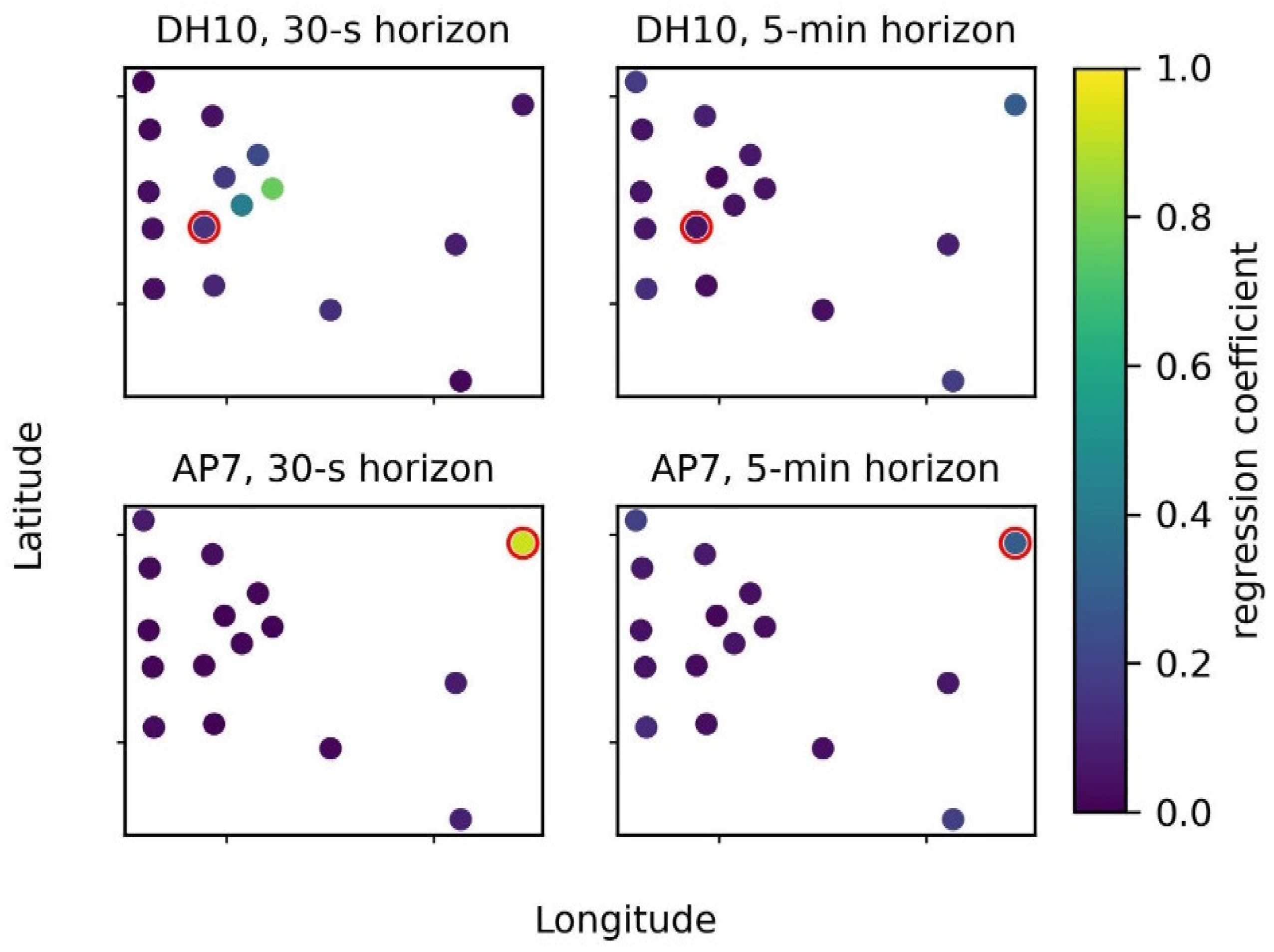
The analysis of the LR coefficients, as illustrated in Figure 9, reinforces this analysis, as has been shown in [58]. For sufficiently short horizons, the presence of adequately distanced upwind stations plays a pivotal role in enhancing the forecasting performance. Conversely the absence of such stations leads to a spatio-temporal model that exhibits minimal deviation from a purely autoregressive approach (Figure 9, left column). On the other hand, for longer horizons, the diminishing autocorrelation factor of the target variable leads to the LR model behaving similarly to a simple spatial average. However, even in this scenario, it still outperforms the baseline smart persistence (Figure 9, right column), likely due to the spatial smoothing effect and resulting mitigation of higher-magnitude errors [58]. This second pattern has also been discussed in Lorenzo et al. [15].
Based on these results, the following sections will focus on the stations ap7 and dh10 (presented in Figure 2) and the 30 s and 5 min horizons, since these represent the main different dynamics found in the data.

3.3. Benchmarking Tree-Based Methods against Linear Regression

Before delving into the impact of stationarizing the irradiance inputs for the various models considered in this study, it is important to first understand the inherent variability in performance across the models in the absence of this preprocessing step.
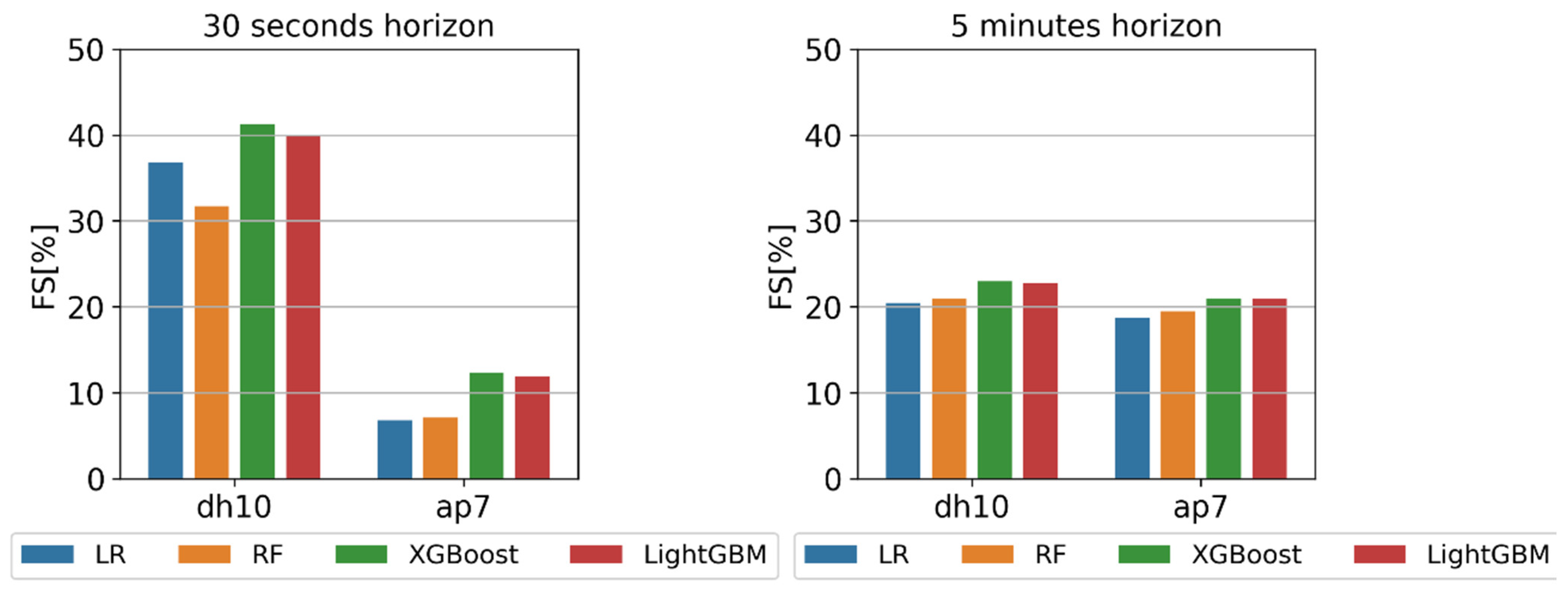
As shown in Figure 10, all the models demonstrate a positive FS for both locations and forecasting horizons, surpassing the baseline reference. XGBoost consistently outperforms all the other models, followed by LightGBM, which is a considerably lighter model but only slightly less performant. Interestingly, the LR emerges as the third best-performing model for short horizons (although the difference is more significant for the dh10 station, which has a close-by upwind neighbor), surpassing the Random Forest (RF) approach. This finding appears to contradict the results reported by Eschenbach et al. [18], where the RF outperforms the LR and is comparable to other ML-based approaches. However, it is important to note that there are some methodological aspects that may differ, but the authors do not provide enough information to fully replicate their study and further pursue this. Namely, the range of values tested for the hyperparameters, or the optimization procedure and resulting optimal configuration.
Overall, the XGBoost leads to similar relative improvements in the FS for both stations compared to the LR model. Notably, these improvements seem to be more pronounced for shorter horizons, where the timescale range is more compatible with the spatial footprint of the sensor network (improvement of 3.2–4.3 PPs in the FS for 10 s ahead, 2.2–2.5 PPs for 5 min ahead). Additionally, the FS for the LightGBM approach, despite being lighter and faster to train, seems to be only 1 PP less performant than XGBoost.

3.4. Impact of Input Stationarization

When considering the stationarization of the irradiance inputs for the tested models, Figure 11 shows that using K t or K c as an input instead of the GHI generally leads to modest accuracy gains (up to 2.5 PPs, see Annexes C and D for the absolute FS values in visual and table formats, instead of the FS variations).
In general, the 5 min horizon tends to benefit more and in a more consistent manner across the models from the input stationarization (1.2 to 2.5 PPs vs. −0.4 to 1.7 PPs). This is likely related to the more uniform performance across the models when using the GHI as input and the higher RMSE for the baseline persistence found for larger horizons (Figure 6), leaving more room for improvement. It is also possible that the stationarization is more impactful when the model focuses on larger-scale weather patterns.
When focusing on the inter-model variations, it appears that ML models, which can capture non-linear patterns, seem to benefit more from this preprocessing step. Conversely, the LR models show almost negligible (and even slightly negative) FS variations for the 30 s horizon. This discrepancy may be attributed to the fact that linear models cannot extract the full benefit of stationarizing the time series, while training the model to minimize the error for K t or K c may overlook the fact that the effective magnitude of the prediction errors irradiance-wise depends on the time of the day (i.e., the value of the top-of-the-atmosphere or clear-sky irradiance). In practice, and as a simplistic illustration, training a model based on irradiance tends to prioritize the minimization of errors close to noon rather than in the early morning or late afternoon.
Lastly, it seems that ML models, and in particular for the shorter-term horizon, benefit more from clear-sky stationarization; otherwise, the models seem to benefit slightly more from top-of-the-atmosphere stationarization. This may be related to the uncertainties associated with the clear-sky modeling (i.e., assuming aerosol and water vapor concentration, as well as the modeling of the resulting attenuation), which in the second case have persisted further in time and may have a detrimental impact in the forecasting accuracy that hampers the potential added value of its embedded information.

3.5. Impact of Including Sun Apparent Position Data

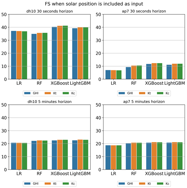
It is of interest to evaluate the impact of the Sun elevation and Sun azimuth angles, as these factors are the primary drivers of the daily and intra-annual seasonality of solar irradiance. The inclusion of this information may yield effects similar to stationarization, since it allows the model to recognize seasonal cycles—specifically, the correlation between the solar profiles and the Sun’s apparent position; at the same time, it may further enhance a forecast model using stationarized solar inputs, since there may be predictable weather patterns intrinsic to the data (e.g., morning clouds). The results are shown in Figure 12.
The results are shown in Figure 12. The RF is the model that shows the biggest improvement after the inclusion of the Sun elevation and Sun azimuth data, with improvements between 3 and 4 PPs in the forecast skill for 30 s ahead. Despite this, the RF still performs worse than or the same as the other ML-based approaches; the RF only surpasses the LR approach for station ap7, where no upwind neighbors are available, and for station dh10 for the 5 min horizon, when the timescale surpasses the sensor network spatial coverage. This increase in the FS and the lower performance found in the previous section seem to point out that even when stationarized inputs are considered, this model still needs information regarding the apparent position of the Sun.
Except for the RF, the models only seem to benefit from this additional information when the GHI is used as input. Looking at the ΔFS and the actual FS values (see Annexes E and F for visual and table formats), the results show that this information can help models handle the lack of solar input stationarization; however, in the presence of stationarized solar inputs, this additional information adds no value to the forecast (variation below 0.1 PP) except for the RF (1 PP increase when both the GHI stationarization and Sun apparent position is considered).

4. Conclusions

This work addresses the stationarization of the global horizontal irradiance (GHI) inputs within the scope of very-short-term spatio-temporal forecasting. It considers a wide range of statistical approaches, including linear regression, Random Forest, and two implementations of Gradient Boosting. Despite the common practice of including this preprocessing step for the input data of such models, there has been no quantitative analysis of its implications for solar-forecasting accuracy. For this, a dataset from the NREL was considered, comprising 17 pyranometers spread over an area of 1 km2 and measuring every 1 s throughout 19 months (although the data were averaged to 10 s to reduce undesirable noise).
The behavior and performance of spatio-temporal solar-forecasting approaches is highly dependent on the spatial distribution of the time series and the spatio-temporal scale at hand. For forecast horizons in the scale of seconds, the achieved performance gains are greatly dependent on the availability of upwind neighbors, since in the absence of such information, the persistence baseline is highly performing (due to its high autocorrelation factor). For longer horizons in the scale of minutes, the temporal scale surpassed what the sensor network, with its limited spatial coverage, could address. However, as persistence approaches degrade, spatially distributed solar information can capture the larger-scale state of the atmosphere and provide performance gains (mostly by producing smoother forecasts).
Concerning the stationarization of solar irradiance inputs, its impact was shown to be relatively dependent on the forecasting model and spatio-temporal context. The persistence approach showed no visible impacts from replacing the GHI with the clearness or the clear-sky indices. For short horizons, the intrinsic lag of a persistence forecast only introduces small-magnitude errors, which are downplayed by a metric such as the nRMSE. However, the remaining models showed different outcomes, achieving gains in the forecast skill for all the cases except for the 30 s horizon linear regression. This seems to indicate that for this horizon, where sharper, more localized spatio-temporal correlations are present, the stationary indices bring to light non-linear atmospheric patterns that drive ML models to perform better. Overall, improvements of between 0.25 and 2.5 PPs were found, with the impact being bigger for contexts where the linear model performs worse (i.e., the more obvious spatio-temporal correlations are less present). For the station AP7, which has no upwind sensors, and a 30 s horizon and for both stations in the 5 -min case, the improvements range from 1 to 2.5 PPs.
Including the solar elevation and azimuth angles seems to compensate for the lack of stationarized solar inputs, highlighting how that information allows the models to distinguish the daily and seasonal variability from the shorter-term, atmosphere-dependent one. However, apart from the underperforming RF model, the models using stationarized inputs seem to obtain no benefit from this information. This might indicate that for the location under study, no pattern relates solar variability to the apparent position with the Sun or that it is already captured by the spatially distributed solar time series.
However, it is also important to note that these results only consider data from one location and particular climate. While the lack of publicly available, highly resolved and spatially distributed irradiance datasets makes it difficult to understand how generalizable the conclusions drawn are, some qualitative discussion can nonetheless take place. On the one hand, we believe that for locations with an equally variable solar resource but less prevailing wind regimes, the spatio-temporal approaches used would perform worse (due to the lower spatio-temporal correlation between sites). However, it seems plausible that in a context with less information available, the relative importance of the detrending and the solar position would increase. For locations with a more stable resource, this information can be particularly relevant to identifying time-dependent weather patterns (e.g., morning fog).
Future works could expand on the range of spatio-temporal scales considered, as well as the models tested, including Artificial Neural Networks with different levels of complexity. If, for example, satellite data were to be considered, it would be possible to explore this topic under various climates at the expense of a more coarse spatio-temporal resolution. Additionally, it would be pertinent to consider datasets where the plane-of-array is non-horizontal or variable across the sensor network, since this impacts the relative impact of a given change in cloud cover (due to its impact in the ratio between direct and diffuse irradiance).
It is also important to mention that such study is transferable to remote-sensing data (e.g., satellite-derived solar irradiance). The expected increase in spatio-temporal resolution with new satellites to come is expected to increase the availability of high-resolution solar data, which are currently highly limited by the considerable costs of deploying and maintaining ground sensor networks. Additionally, while additional weather variables such as the temperature or humidity have little to no impact on the irradiance seasonality addressed in this work, including such data as complementary inputs could further improve the forecasting performance.

Author Contributions

Conceptualization, R.A.e.S. and L.B.C.; formal analysis, L.B.C., R.A.e.S., M.Á.M.C. and C.-I.C.; investigation, L.B.C.; methodology, L.B.C. and R.A.e.S.; resources, R.A.e.S., M.Á.M.C. and C.-I.C.; supervision, R.A.e.S., M.Á.M.C. and C.-I.C.; validation, L.B.C. and R.A.e.S.; visualization, L.B.C.; writing—original draft, L.B.C. and R.A.e.S.; writing—review and editing, L.B.C., R.A.e.S., M.Á.M.C. and C.-I.C. All authors have read and agreed to the published version of the manuscript.

Funding

This research received no external funding.

Data Availability Statement

This work was based on a public dataset provided by the National Renewable Energy Laboratory. The data are freely available at http://www.nrel.gov/midc/oahu_archive/ (accesed on 2 August 2023).

Conflicts of Interest

The authors declare no conflicts of interest.

Appendix A. Mean Absolute Error (MAE) Results Obtained from ap7 and dh10 Sensors

MAEStationap7dh10
Horizon TargetGHIKcKtGHIKcKt
Model
30 s LR 65.1163.6764.3838.4438.7738.67
RF 65.4664.9464.4542.7942.0642.24
LightGBM61.5760.0159.2237.5436.3236.54
XGBoost 60.2758.9658.5035.2734.3934.47
5 min LR 133.99132.00132.70124.07121.29122.51
RF 133.39128.82129.90124.11120.06121.18
LightGBM 129.85124.84125.51120.53116.15116.66
XGBoost 129.06124.57125.00119.92115.42116.11

Appendix B. Determination Coefficient (R2) Results Obtained from ap7 and dh10 Sensors

R2Stationap7dh10
Horizon TargetGHIKcKtGHIKcKt
Model
30 s LR 0. 840. 840. 840. 930. 930. 93
RF 0.830.840.840.870.910.91
LightGBM0.850.860.860.930.930.93
XGBoost 0.840.860.860.880.940.94
5 min LR 0.630.650.650.650.660.66
RF 0.630.650.660.650.670.67
LightGBM 0.650.670.670.670.680.68
XGBoost 0.650.670.670.670.680.68

Appendix C. FS Values for Different Variations of the Solar Irradiance Input

Energies 17 03527 i001

Appendix D. Forecast Skill (FS) Results Obtained from ap7 and dh10 Sensors

FSStationap7dh10
Horizon TargetGHIKtKcGHIKtKc
Model
30 s LR 6.546.84 6.8237.15 36.97 36.78
RF 6.107.29 7.0831.55 32.17 31.69
LightGBM 10.17 11.67 11.90 39.21 39.9240.01
XGBoost 10.85 12.1412.37 40.34 41.16 41.27
5 min LR 16.76 18.5318.6719.21 20.58 20.44
RF 17.13 19.63 19.46 19.45 21.52 20.96
LightGBM 18.83 21.17 20.92 21.07 23.13 22.70
XGBoost 19.24 21.1821.00 21.41 23.18 22.95

Appendix E. FS Values for Different Variations of the Solar Irradiance Input When the Sun Position Is Also Considered
Energies 17 03527 i002

Appendix F. FS Results Obtained from ap7 and dh10 Sensors When Solar Position Is Included as Input

FSStationap7dh10
Horizon TargetGHIKcKtGHIKcKt
Model
30 s LR 6.96 6.82 6.89 37.15 36.88 37.04
RF 9.32 10.48 10.46 34.91 35.68 35.60
LightGBM11.08 11.87 11.85 39.23 39.95 40.08
XGBoost 11.70 12.34 12.35 40.30 41.22 41.10
5 min LR 18.72 18.67 18.67 20.62 20.53 20.56
RF 20.31 20.63 20.70 22.14 22.36 22.46
LightGBM 20.74 21.00 21.12 22.51 22.93 23.08
XGBoost 20.68 20.96 21.12 22.46 22.90 22.94

References

  1. Gandhi, O.; Zhang, W.; Kumar, D.S.; Rodríguez-Gallegos, C.D.; Yagli, G.M.; Yang, D.; Reindl, T.; Srinivasan, D. The value of solar forecasts and the cost of their errors: A review. Renew. Sustain. Energy Rev. 2024, 189, 113915. [Google Scholar] [CrossRef]
  2. Yang, D.; Wang, W.; Gueymard, C.A.; Hong, T.; Kleissl, J.; Huang, J.; Perez, M.J.; Perez, R.; Bright, J.M.; Xia, X.; et al. A review of solar forecasting, its dependence on atmospheric sciences and implications for grid integration: Towards carbon neutrality. Renew. Sustain. Energy Rev. 2022, 161, 112348. [Google Scholar] [CrossRef]
  3. Boland, J. Spatial-temporal forecasting of solar radiation. Renew. Energy 2015, 75, 607–616. [Google Scholar] [CrossRef]
  4. Singla, P.; Duhan, M.; Saroha, S. Different normalization techniques as data preprocessing for one step ahead forecasting of solar global horizontal irradiance. In Artificial Intelligence for Renewable Energy Systems; Elsevier: Amsterdam, The Netherlands, 2022; pp. 209–230. [Google Scholar] [CrossRef]
  5. Hollands, K.G.T. A derivation of the diffuse fraction’s dependence on the clearness index. Sol. Energy 1985, 35, 131–136. [Google Scholar] [CrossRef]
  6. Perez, R.; Ineichen, P.; Seals, R.; Zelenka, A. Making full use of the clearness index for parameterizing hourly insolation conditions. Sol. Energy 1990, 45, 111–114. [Google Scholar] [CrossRef]
  7. Blanc, P.; Wald, L. On the intraday resampling of time-integrated values of solar radiation. In Proceedings of the 10th EMS Annual Meeting (European Meteorological Society), Zurich, Switzerland, 13–17 September 2010. [Google Scholar]
  8. Grantham, A.P.; Pudney, P.J.; Ward, L.A.; Belusko, M.; Boland, J.W. Generating synthetic five-minute solar irradiance values from hourly observations. Sol. Energy 2017, 147, 209–221. [Google Scholar] [CrossRef]
  9. Gueymard, C.A.; Bright, J.M.; Lingfors, D.; Habte, A.; Sengupta, M. A posteriori clear-sky identification methods in solar irradiance time series: Review and preliminary validation using sky imagers. Renew. Sustain. Energy Rev. 2019, 109, 412–427. [Google Scholar] [CrossRef]
  10. Suárez-García, A.; Díez-Mediavilla, M.; Granados-López, D.; González-Peña, D.; Alonso-Tristán, C. Benchmarking of meteorological indices for sky cloudiness classification. Sol. Energy 2020, 195, 499–513. [Google Scholar] [CrossRef]
  11. Shepero, M.; Munkhammar, J.; Widén, J. A generative hidden Markov model of the clear-sky index. J. Renew. Sustain. Energy 2019, 11, 043703. [Google Scholar] [CrossRef]
  12. Lohmann, G. Irradiance Variability Quantification and Small-Scale Averaging in Space and Time: A Short Review. Atmosphere 2018, 9, 264. [Google Scholar] [CrossRef]
  13. Engerer, N.A.; Mills, F.P. KPV: A clear-sky index for photovoltaics. Sol. Energy 2014, 105, 679–693. [Google Scholar] [CrossRef]
  14. Oh, M.; Kim, C.K.; Kim, B.; Yun, C.; Kang, Y.-H.; Kim, H.-G. Spatiotemporal Optimization for Short-Term Solar Forecasting Based on Satellite Imagery. Energies 2021, 14, 2216. [Google Scholar] [CrossRef]
  15. Lorenzo, A.T.; Holmgren, W.F.; Cronin, A.D. Irradiance forecasts based on an irradiance monitoring network, cloud motion, and spatial averaging. Sol. Energy 2015, 122, 1158–1169. [Google Scholar] [CrossRef]
  16. Lauret, P.; Alonso-Suárez, R.; Le Gal La Salle, J.; David, M. Solar Forecasts Based on the Clear Sky Index or the Clearness Index: Which Is Better? Solar 2022, 2, 432–444. [Google Scholar] [CrossRef]
  17. Yang, D. Choice of clear-sky model in solar forecasting. J. Renew. Sustain. Energy 2020, 12, 026101. [Google Scholar] [CrossRef]
  18. Eschenbach, A.; Yepes, G.; Tenllado, C.; Gomez-Perez, J.I.; Pinuel, L.; Zarzalejo, L.F.; Wilbert, S. Spatio-Temporal Resolution of Irradiance Samples in Machine Learning Approaches for Irradiance Forecasting. IEEE Access 2020, 8, 51518–51531. [Google Scholar] [CrossRef]
  19. De Paiva, G.M.; Pimentel, S.P.; Alvarenga, B.P.; Marra, E.G.; Mussetta, M.; Leva, S. Multiple site intraday solar irradiance forecasting by machine learning algorithms: MGGP and MLP neural networks. Energies 2020, 13, 3005. [Google Scholar] [CrossRef]
  20. Ineichen, P.; Perez, R. A new airmass independent formulation for the Linke turbidity coefficient. Sol. Energy 2002, 73, 151–157. [Google Scholar] [CrossRef]
  21. Lefèvre, M.; Oumbe, A.; Blanc, P.; Espinar, B.; Gschwind, B.; Qu, Z.; Wald, L.; Schroedter-Homscheidt, M.; Hoyer-Klick, C.; Arola, A.; et al. McClear: A new model estimating downwelling solar radiation at ground level in clear-sky conditions. Atmos. Meas. Tech. 2013, 6, 2403–2418. [Google Scholar] [CrossRef]
  22. Gueymard, C.A. REST2: High-performance solar radiation model for cloudless-sky irradiance, illuminance, and photosynthetically active radiation—Validation with a benchmark dataset. Sol. Energy 2008, 82, 272–285. [Google Scholar] [CrossRef]
  23. Haurwitz, B. Insolation in relation to cloudiness and cloud density. J. Meteorol. 1945, 2, 154–166. [Google Scholar] [CrossRef]
  24. Amaro e Silva, R. Spatio-Temporal Solar Forecasting; Universidade de Lisboa, Lisboa, Portugal. 2019. Available online: http://hdl.handle.net/10451/47449 (accessed on 23 January 2022).
  25. Benavides Cesar, L.; Silva, R.A.E.; Callejo, M.Á.M.; Cira, C.I. Review on Spatio-Temporal Solar Forecasting Methods Driven by In Situ Measurements or Their Combination with Satellite and Numerical Weather Prediction (NWP) Estimates. Energies 2022, 15, 4341. [Google Scholar] [CrossRef]
  26. Voyant, C.; Notton, G.; Kalogirou, S.; Nivet, M.-L.; Paoli, C.; Motte, F.; Fouilloy, A. Machine learning methods for solar radiation forecasting: A review. Renew. Energy 2017, 105, 569–582. [Google Scholar] [CrossRef]
  27. Segupta, M.; Andreas, A. Oahu Solar Measurement Grid (1-Year Archive): 1-Second Solar Irradiance; Oahu, Hawaii (Data); National Renewable Energy Lab. (NREL): Golden, CO, USA, 2010. [Google Scholar] [CrossRef]
  28. Yang, D.; Ye, Z.; Lim, L.H.I.; Dong, Z. Very short term irradiance forecasting using the lasso. Sol. Energy 2015, 114, 314–326. [Google Scholar] [CrossRef]
  29. Aryaputera, A.W.; Yang, D.; Zhao, L.; Walsh, W.M. Very short-term irradiance forecasting at unobserved locations using spatio-temporal kriging. Sol. Energy 2015, 122, 1266–1278. [Google Scholar] [CrossRef]
  30. Amaro E Silva, R.; Haupt, S.E.; Brito, M.C. A regime-based approach for integrating wind information in spatio-temporal solar forecasting models. J. Renew. Sustain. Energy 2019, 11, 056102. [Google Scholar] [CrossRef]
  31. Jiao, X.; Li, X.; Lin, D.; Xiao, W. A Graph Neural Network Based Deep Learning Predictor for Spatio-Temporal Group Solar Irradiance Forecasting. IEEE Trans. Ind. Inform. 2022, 18, 6142–6149. [Google Scholar] [CrossRef]
  32. Yang, D.; Yagli, G.M.; Srinivasan, D. Sub-minute probabilistic solar forecasting for real-time stochastic simulations. Renew. Sustain. Energy Rev. 2022, 153, 111736. [Google Scholar] [CrossRef]
  33. Widén, J.; Shepero, M.; Munkhammar, J. On the properties of aggregate clear-sky index distributions and an improved model for spatially correlated instantaneous solar irradiance. Sol. Energy 2017, 157, 566–580. [Google Scholar] [CrossRef]
  34. Munkhammar, J.; Widén, J.; Hinkelman, L.M. A copula method for simulating correlated instantaneous solar irradiance in spatial networks. Sol. Energy 2017, 143, 10–21. [Google Scholar] [CrossRef]
  35. Munkhammar, J. Very short-term probabilistic and scenario-based forecasting of solar irradiance using Markov-chain mixture distribution modeling. Sol. Energy Adv. 2024, 4, 100057. [Google Scholar] [CrossRef]
  36. Hinkelman, L.M. Differences between along-wind and cross-wind solar irradiance variability on small spatial scales. Sol. Energy 2013, 88, 192–203. [Google Scholar] [CrossRef]
  37. Blanc, P.; Wald, L. The SG2 algorithm for a fast and accurate computation of the position of the Sun for multi-decadal time period. Sol. Energy 2012, 86, 3072–3083. [Google Scholar] [CrossRef]
  38. Blanc, P.; Wald, L. Solar Geometry 2. Available online: https://github.com/gschwind/sg2 (accessed on 3 May 2022).
  39. Gschwind, B.; Wald, L.; Blanc, P.; Lefèvre, M.; Schroedter-Homscheidt, M.; Arola, A. Improving the McClear model estimating the downwelling solar radiation at ground level in cloud-free conditions—McClear-v3. Meteorol. Zeitschrift 2019, 28, 147–163. [Google Scholar] [CrossRef]
  40. Holmgren, W.F.; Hansen, C.W.; Mikofski, M.A. pvlib python: A python package for modeling solar energy systems. J. Open Source Softw. 2018, 3, 884. [Google Scholar] [CrossRef]
  41. CAMS Solar Radiation Time-Series. Copernicus Atmosphere Monitoring Service (CAMS) Atmosphere Data Store (ADS). Available online: https://ads.atmosphere.copernicus.eu/cdsapp#!/dataset/cams-solar-radiation-timeseries?tab=overview (accessed on 3 May 2022).
  42. Amaro e Silva, R.; Brito, M.C. Spatio-temporal PV forecasting sensitivity to modules’ tilt and orientation. Appl. Energy 2019, 255, 113807. [Google Scholar] [CrossRef]
  43. Dambreville, R.; Blanc, P.; Chanussot, J.; Boldo, D. Very short term forecasting of the global horizontal irradiance using a spatio-temporal autoregressive model. Renew. Energy 2014, 72, 291–300. [Google Scholar] [CrossRef]
  44. Gagne, D.J.; McGovern, A.; Haupt, S.E.; Williams, J.K. Evaluation of statistical learning configurations for gridded solar irradiance forecasting. Sol. Energy 2017, 150, 383–393. [Google Scholar] [CrossRef]
  45. Breiman, L. Random Forests. Mach. Learn. 2001, 45, 5–32. [Google Scholar] [CrossRef]
  46. James, G.; Witten, D.; Hastie, T.; Tibshirani, R.; Thaylor, J. An Introduction to Statistical Learning with Applications in Python; Springer: New York, NY, USA, 2023; ISBN 9781461471370. [Google Scholar]
  47. Chen, T.; Guestrin, C. XGBoost: A scalable tree boosting system. In Proceedings of the 22nd ACM SIGKDD International Conference on Knowledge Discovery and Data Mini, San Francisco, CA, USA, 13–17 August 2016; pp. 785–794. [Google Scholar] [CrossRef]
  48. Ke, G.; Meng, Q.; Finley, T.; Wang, T.; Chen, W.; Ma, W.; Ye, Q.; Liu, T.Y. LightGBM: A highly efficient gradient boosting decision tree. In Proceedings of the 31st International Conference on Neural Information Processing Syste, Long Beach, CA, USA, 4–9 December 2017; pp. 3147–3155. [Google Scholar]
  49. Pedregosa, F.; Varoquaux, G.; Gramfort, A.; Michel, V.; Thirion, B.; Grisel, O.; Blondel, M.; Müller, A.; Nothman, J.; Louppe, G.; et al. Scikit-learn: Machine Learning in Python. J. Mach. Learn. Res. 2011, 12, 2825–2830. Available online: http://jmlr.csail.mit.edu/papers/v12/pedregosa11a.html%5Cnhttp://arxiv.org/abs/1201.0490 (accessed on 5 February 2024).
  50. GitHub. XGBoost. Available online: https://github.com/dmlc/xgboost (accessed on 10 January 2022).
  51. GitHub. LightGBM. Available online: https://github.com/Microsoft/LightGBM (accessed on 10 January 2022).
  52. Kim, S.G.; Jung, J.Y.; Sim, M.K. A two-step approach to solar power generation prediction based on weather data using machine learning. Sustainability 2019, 11, 1501. [Google Scholar] [CrossRef]
  53. Carrera, B.; Kim, K. Comparison analysis of machine learning techniques for photovoltaic prediction using weather sensor data. Sensors 2020, 20, 3129. [Google Scholar] [CrossRef] [PubMed]
  54. Feng, C.; Zhang, J. SolarNet: A deep convolutional neural network for solar forecasting via sky images. In Proceedings of the 2020 IEEE Power & Energy Society Innovative Smart Grid Technologies Conference (ISGT), Washington, DC, USA, 17–20 February 2020. [Google Scholar] [CrossRef]
  55. Marquez, R.; Coimbra, C.F.M. Proposed Metric for Evaluation of Solar Forecasting Models. J. Sol. Energy Eng. 2013, 135, 011016. [Google Scholar] [CrossRef]
  56. Yang, D.; Alessandrini, S.; Antonanzas, J.; Antonanzas-Torres, F.; Badescu, V.; Beyer, H.G.; Blaga, R.; Boland, J.; Bright, J.M.; Coimbra, C.F.M.; et al. Verification of deterministic solar forecasts. Sol. Energy 2020, 210, 20–37. [Google Scholar] [CrossRef]
  57. Yang, D.; Kleissl, J.; Gueymard, C.A.; Pedro, H.T.C.; Coimbra, C.F.M. History and trends in solar irradiance and PV power forecasting: A preliminary assessment and review using text mining. Sol. Energy 2018, 168, 60–101. [Google Scholar] [CrossRef]
  58. Amaro e Silva, R.; Brito, M.C. Impact of network layout and time resolution on spatio-temporal solar forecasting. Sol. Energy 2018, 163, 329–337. [Google Scholar] [CrossRef]
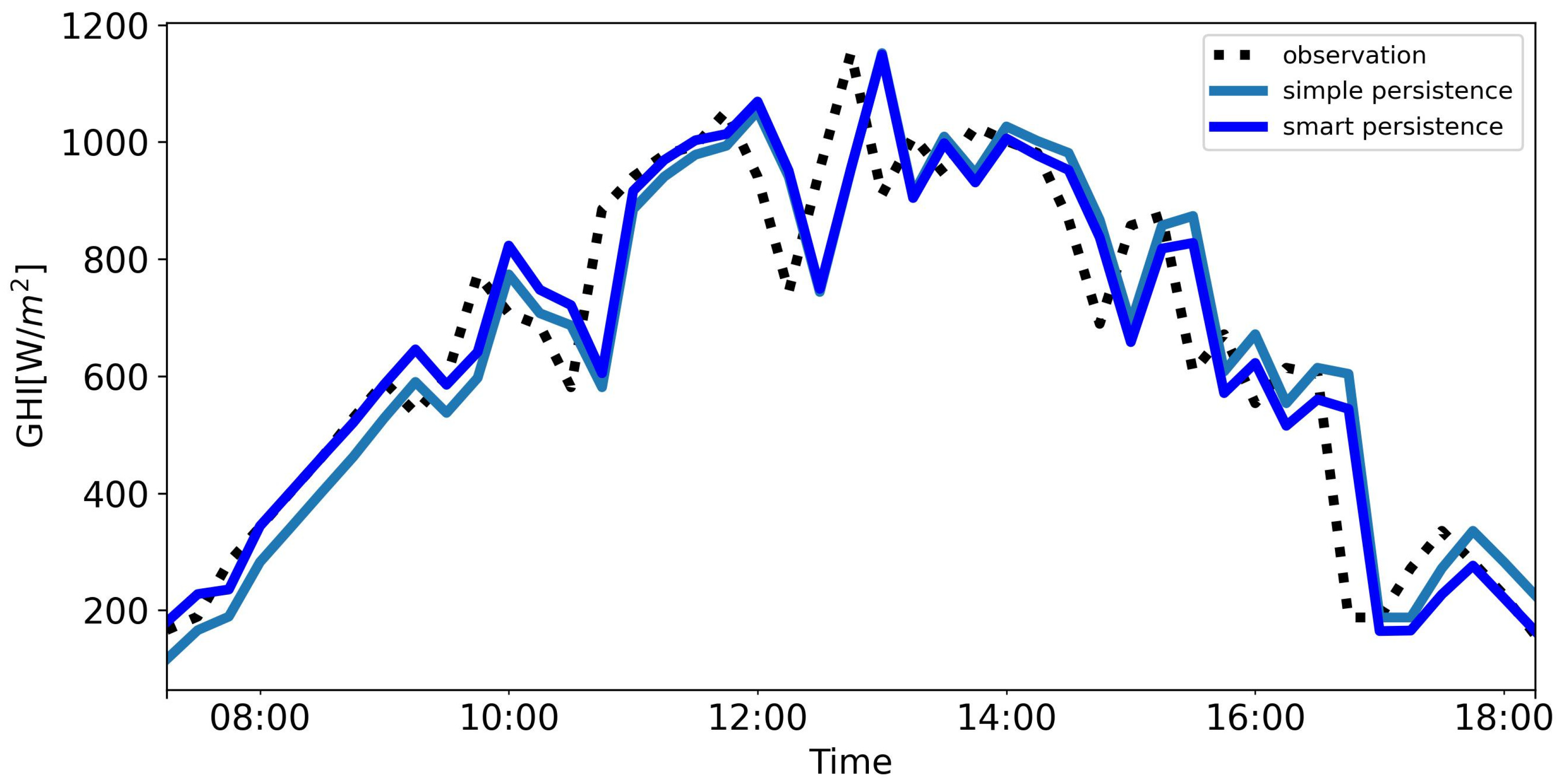
Figure 1. Example of a simple persistence forecast and its delay. Note that the persisting previous observations of a non-stationary variable fail to capture the data’s daily seasonality.
Energies 17 03527 g001
Figure 2. Spatial distribution of the pyranometers that comprise the Oahu Solar Measurement Grid from Hawaii [27], which is considered in this work.
Energies 17 03527 g002
Figure 3. Representation of Random Forest trees, consisting of a set of parallel regression trees each computing a prediction, from which the average of the ensemble is taken as the final output.
Energies 17 03527 g003
Figure 4. Representation of the tree growth in the XGBoost (top) and LightGBM (bottom) models. Notes: (1) In each iteration, either all or a single leaf node is expanded, depending on the growth strategy. (2) The number of leaf nodes grows considerably faster in the first case, making it computationally more expensive.
Energies 17 03527 g004
Figure 5. Schema describing the input–output flow of the models considered. Note: Whereas the persistence approaches only considered the more recent data of the target under study, the remaining approaches exploit the three latest data points from each station at once.
Energies 17 03527 g005
Figure 6. Root mean squared error (RMSE) distribution for the simple and smart persistence models across the various stations and 30 s (left) and 5 min (right) horizons, with all the models performing similarly for each horizon. Note the shift in the y-axis on the right plot, with the RMSE increasing by almost a factor of 2 due to the longer horizon.
Energies 17 03527 g006
Figure 7. Range of forecast skill in the Hawaii dataset for forecast horizons between 10 s and 10 min using an LR approach (median values indicated by the solid line).
Energies 17 03527 g007
Figure 8. Forecast skill for the LR model with a time resolution of 10 s and horizons of 30 s (left) and 5 min (right). Note: Considering the prevailing northeasterly winds driving cloud advection, the left plot highlights how the FS depends on the availability of upwind neighbors (east or northeast) for shorter timescales, whereas all the stations perform similarly once the forecast horizon surpasses the spatial coverage of the sensor network.
Energies 17 03527 g008
Figure 9. Mean absolute regression coefficients when forecasting for the target station (circled in red), indicating the contribution of each station to the LR model. Note: The relevance of upwind sensors for the 30 s model of station DH10 (upper left plot), in contrast to AP7 (bottom left plot), highlights the spatio-temporal dynamics of Oahu, whereas the uniform pattern found in the 5 min models (right column) describe a spatio-temporal average-like approach.
Energies 17 03527 g009
Figure 10. Inter-model comparison for spatio-temporal forecasting using the GHI as input, for the dh10 and ap7 stations, for 30 s and 5 min horizons.
Energies 17 03527 g010
Figure 11. Absolute impact on forecast skill due to the stationarization (to Kt in blue, Kc in orange) of the solar irradiance inputs.
Energies 17 03527 g011
Figure 12. Impact on forecast skill from including the solar elevation and azimuth angles as inputs in the various models, with the various solar inputs, and for the two stations and forecast horizons.
Energies 17 03527 g012
Table 1. Hyperparameters and respective values explored in the training of the Random Forest, XGBoost, and LightGBM models.
ModelHyperparameter Brief DescriptionAssessed Values C
Random Forest“n_estimators”Number of trees in the forest150, 200, 250, 300, 350, 400, 500, 600
“min_samples_leaf”Minimum number of samples in each leaf node0.01, 0.025, 0.05
XGBoost and LightGBM“max_depth”Maximum depth of each tree 5, 10, 15, 20, 25
EtaLearning rate, shrinkage parameter to prevent overfitting0.001, 0.01, 0.1, 0.15, 0.3, 0.45
Disclaimer/Publisher’s Note: The statements, opinions and data contained in all publications are solely those of the individual author(s) and contributor(s) and not of MDPI and/or the editor(s). MDPI and/or the editor(s) disclaim responsibility for any injury to people or property resulting from any ideas, methods, instructions or products referred to in the content.