Assessment of Municipal Waste Forecasting Methods in Poland Considering Socioeconomic Aspects

Abstract

As a public service, municipal waste management at the local and regional levels should be carried out in an environmentally friendly and economically justified manner. Information on the quantity and composition of generated municipal waste is essential for planning activities related to the implementation and optimization of the process. There is a need for reliable forecasts regarding the amount of waste generated in each area. Due to the variability in the waste accumulation rate, this task is difficult to accomplish, especially at the local level. The literature contains many reports on this issue, but there is a lack of studies indicating the preferred method depending on the independent variables, the complexity of the algorithm, the time of implementation, and the quality of the forecast. The results concerning the quality of forecasting methods are difficult to compare due to the use of different sets of independent variables, forecast horizons, and quality assessment indicators. This paper compares the effectiveness of selected forecasting models in predicting the amount of municipal waste collection generated in Polish municipalities. The authors compared nine methods, including artificial neural networks (ANNs), support regression trees (SRTs), rough set theory (RST), multivariate adaptive regression splines (MARS), and random regression forests (RRFs). The analysis was based on 31 socioeconomic indicators for 2451 municipalities in Poland. The Boruta algorithm was used to select significant variables and eliminate those with little impact on forecasting. The quality of the forecasts was evaluated using eight indicators, such as the absolute percentage error (MAPE), mean absolute error (MAE), and coefficient of determination (R²). A comprehensive evaluation of the forecasting models was carried out using the APEKS method. An analysis of the results showed that the best forecasting methods depended on the set of independent variables and the evaluation criteria adopted. Waste management expenditures, the levels of sanitation and housing infrastructure, and the cost-effectiveness of waste management services were key factors influencing the amount of municipal waste. Additionally, this research indicated that adding more variables does not always improve the quality of forecasts, highlighting the importance of proper selection. The use of a variable selection algorithm, combined with the consideration of the impact of various socioeconomic factors on municipal waste generation, can significantly improve the quality of forecasts. The SRT, CHAID, and MARS methods can become valuable tools for predicting municipal waste volumes, which, in turn, will help to improve waste management system.

1. Introduction

Poland, like many other countries around the world, is facing the challenge of increasing amounts of municipal waste. The processing of municipal waste in Poland faces numerous difficulties that pose a serious challenge to sustainable development and environmental protection. A key problem remains the low level of recycling, which significantly deviates from EU requirements. In 2021, only 27% of municipal waste was recycled, while the European Union’s target for 2030 is 50% [1]. Achieving this goal requires decisive action at both the local and national levels. The lack of modern infrastructure for waste processing is another significant barrier. Poland has an insufficient number of recycling plants and waste incineration plants, which leads to the overloading of existing landfills. It is estimated that there are about 1700 landfills in Poland, many of which do not meet EU standards. The construction of new, more efficient waste treatment facilities is necessary to cope with the growing volume of waste and improve the efficiency of waste treatment [1]. The illegal dumping of waste is an additional problem that negatively affects the environment and public health. The lack of effective enforcement and insufficient environmental awareness among part of the population lead to the dumping of waste in forests, along roads, and in other public places. Effectively solving this problem requires tighter controls and increased environmental education. The introduction of more advanced waste treatment technologies, such as waste incinerators and biogas plants, is key to improving the situation. Although investments in these technologies are costly, they can significantly increase the efficiency of waste management and reduce the negative impact of waste on the environment. Waste incinerators can not only reduce the volume of waste going to landfills but also generate energy, which is an additional benefit [2,3]. Waste management, including the operation of incinerators, should prioritize local needs and the ability to transfer and use the energy generated. Combined heat and power (CHP) effectively generate both electricity and heat, serving as an example of an efficient system. Modern thermal waste conversion plants, such as grate incinerators, are a key component of Poland’s municipal waste management sector, especially given the planned expansion of these facilities to address the growing problem of waste generation [4]. Unfortunately, at present, most of the waste collected is sent to landfills, and only a small percentage is thermally converted for energy recovery. To meet the challenges of municipal waste processing, cooperation at all levels of government and public involvement are essential. Effective waste management requires the accurate forecasting of waste volumes and a comprehensive analysis of the factors contributing to waste generation. Increasing consumption and changing social habits have a direct impact on the amount and type of waste generated, which must be considered in planning infrastructure and waste treatment systems [5]. An integrated approach, including both prevention and modernization measures, is necessary for Poland to effectively manage municipal waste and move toward a more sustainable future.

2. A Critical Bibliographic Analysis of Methods for Forecasting the Municipal Waste Accumulation Rate

The aim of this analysis is to compare methods for estimating the municipal waste accumulation rate and their capabilities, strengths, and weaknesses in the examples analyzed.

The accurate forecasting of waste generation is a key aspect of effective waste management. An analysis of various variables, which can be categorized as socio-cultural, environmental, and economic, makes it possible to identify the main factors affecting waste generation [1,2,6,7,8,9,10]. The most commonly used groups of predictors in the literature for estimating the waste accumulation rate can be divided into socio-cultural, environmental, and economic variables, as summarized in

Table 1. Independent variables related to the prediction of municipal waste volumes.

No.	Independent Variables		Reference
1.	Socio-cultural	age cultural factors demographic conditions education	[6,8,10,11,12,13,14,15,16]
2.	Environmental	energy consumption precipitation temperature	[1,17,18,19,20,21,22,23]
3.	Economic	economic trends employment rate household income work and occupation	[10,12,17,24,25,26,27,28,29]

.

Predicting the amount of municipal waste is a task with a high degree of uncertainty, which is an important part of the decision-making process in waste management [29,30]. The proper identification and selection of modeling variables are very important to avoid over-fitting the model and to facilitate the interpretation of the results, which, in turn, increases their reliability [11]. The level of detail in the analysis and the accompanying uncertainty are key elements to consider. The data used to create predictive models can be imperfect, containing missing values, inconsistencies, noise, and outliers [30]. The lack of reliable data further hinders accurate forecasting, forcing the search for alternative sources of information [16,31,32].

The accurate forecasting of the amount of municipal waste generated is fundamental to effective waste management. The proper modeling of waste flows and the careful selection of modeling variables are essential to achieving accurate and reliable forecasts. This forms the foundation for effective infrastructure planning and waste reduction strategies, especially for energy recovery initiatives. The choice of modeling technique and the consideration of exogenous factors vary considerably by country, regional specificity, and level of development. Models based on statistical methods such as linear and multiple regression [15,28,29], fuzzy and rough set theories [7,33,34,35], multivariate gray models [36], time series [37,38,39], and artificial neural networks [7,10,15,17,21,27,30,31,39,40,41,42,43,44,45,46] are used to forecast municipal waste generation. Numerous studies emphasize that the lack of sufficient data on municipal waste forecasting and management is a significant obstacle to the development of effective waste management systems [7,34]. An analysis of the above-mentioned literature items showed that it is difficult to compare the presented results with each other and choose the best method for forecasting the municipal waste accumulation rate due to different sets of independent variables, different forecast horizons, and different quality assessment indicators, as well as the lack of comprehensive assessment due to the simultaneous consideration of several assessment criteria. Therefore, it is necessary to continue research in this area to develop more precise and effective methods for forecasting municipal waste volumes and effectively managing this important aspect of the sustainable development of societies [1,11,27,32].

The purpose of this study was to evaluate the effectiveness of the selected methods in forecasting the amount of municipal waste collected on an annual basis based on socioeconomic factors. The study was conducted on 2451 municipalities in Poland. In the study, random forest methods available in the Boruta package [47,48,49] were used to select sets of independent variables. For the selected sets of variables, effective methods were sought to predict the municipal waste collection rate. The choice of the preferred method depended heavily on the evaluation criteria adopted. The multi-criteria APEKS method [50] was used to select the best model or group of models for a specific set of independent variables.

3. Materials and Methods

The research material included 31 socioeconomic indicators describing the total amount of municipal waste generated in 2477 municipalities in Poland. The data for the analysis were obtained from the Central Statistical Office in Poland [51] and from the paper by Bański [52], which describes the typology of the municipalities covered by the study. In the first stage, a preliminary data selection was carried out, involving the removal of incomplete observations. After this operation, 2451 municipalities remained for further analysis. Subsequently, methods for forecasting the amount of municipal waste were selected. Nine methods, differing in their approach to building a forecasting model, were arbitrarily chosen. These methods included artificial neural networks (ANNs), exhaustive regression trees (CHAID), general regression trees (CART), k-nearest neighbors (KNN), multivariate adaptive regression splines (MARS), random regression forests (RRFs), rough set theory (RST), support regression trees (SRTs), and support vector machines (SVMs). The processes of constructing the structure and then teaching the developed artificial neural network were performed in the Statistica 13 program. The neural networks analyzed thus had between 4 and 11 neurons in the input layer and 1 neuron in the output layer. The study used linear, logistic, hyperbolic, and exponential functions to activate the hidden and output layers. During the construction of the network, not only the type of activation function but also the number of neurons in the hidden layer was changed. This part of the study used an algorithm implemented in Statistica, which searched for the optimal network structure by varying the number of neurons in the hidden layer from 2 to 15. Three learning algorithms were used in the study, i.e., coupled gradients, fastest gradient, and the Broyden–Fletcher–Goldfarb–Shanno (BFGS) algorithm. The error rate, which is the sum of the squares of the differences between the actual values of the predicted variable and the values of the independent variable and the values obtained at the output neuron, was used to assess the quality of the neural network during iterative learning. In the MARS method, the maximum number of basis functions was limited to 22. No interactions between variables were used, and a level 2 penalty was applied for introducing another basis function into the model. In order to prevent the model from overlearning, the CART, CHAID, SVM, and KNN methods used v-fold cross-validation. This method consists of repeating the procedure of partitioning the input dataset into learning and test subsets on which the models are based. By assessing their quality in each iteration, we can complete the model-building process without the model overlearning. In the case of overlearning, the model has a very low error on the learning set, but no predictive ability on the new data. Metrics such as the absolute percentage error (APE), mean absolute error (MAE), mean error (ME), mean absolute percentage error (MAPE), mean percentage error (MPE), mean bias error (MBE), coefficient of variation of root mean square error (CV RMSE), and coefficient of determination (R²) were used to evaluate the performance of these methods [53]. The evaluation metrics were determined using Equations (1)–(8):

$$CV RMSE={\displaystyle \frac{\sqrt{{\sum }_{m=1}^{n_g}\frac{{\left(y_i-y_i^P\right)}^2}{y_i}}}{\frac{1}{n_g} {\sum }_{m=1}^{n_g}{y}_i}}·100\% m=1,2,3\dots .n_g$$

(1)

$$MAE={\displaystyle \frac{1}{n_g}}{\displaystyle \sum }_{m=1}^{n_g}\left|y_i-y_i^P\right| m=1,2,3\dots .n_g$$

(2)

$$MAPE={\displaystyle \frac{1}{n_g}}{\displaystyle \sum }_{m=1}^{n_g}\left|{\displaystyle \frac{y_i-y_i^P}{y_i}}\right|·100\% m=1,2,3\dots .n_g$$

(3)

$$MBE=\frac{{\sum }_{m=1}^{n_g}\left(y_i-y_i^P\right)}{{\sum }_{m=1}^{n_g}{y}_i}·100\% m=1,2,3\dots .n_g$$

(4)

$$ME={\displaystyle \frac{1}{n_g}}{\displaystyle \sum }_{m=1}^{n_g}\left(y_i-y_i^P\right) m=1,2,3\dots .n_g$$

(5)

$$MPE={\displaystyle \frac{1}{n_g}}{\displaystyle \sum }_{m=1}^{n_g}\left({\displaystyle \frac{y_i-y_i^P}{y_i}}\right)·100\% m=1,2,3\dots .n_g$$

(6)

$$PE=\left({\displaystyle \frac{y_i-y_i^P}{y_i}}\right)·100\%$$

(7)

$$R^2={\left({\displaystyle \frac{n_g·{\sum }_{m=1}^{n_g}{y}_i·y_i^P-{\sum }_{m=1}^{n_g}{y}_i·{\sum }_{m=1}^{n_g}{y}_i^P}{\sqrt{\left(n_g·{\sum }_{m=1}^{n_g}{y}_i^2-{\left({\sum }_{m=1}^{n_g}{y}_i\right)}^2\right)·\left(n_g·{\sum }_{m=1}^{n_g}{y}_i^{P 2}-{\left({\sum }_{m=1}^{n_g}{y}_i^P\right)}^2\right)}}}\right)}^2$$

(8)

where y_i is the actual value (quantity) in facility i, and y^p_i is the forecast value (quantity) in facility i. The difference between y_i and y^p_i is divided by the actual value y_i and m, the number of the test object (m = $1,2,3$....n_g).

The purposefully selected set of indicators allowed a multi-faceted assessment of the quality of the forecasts developed with the compared multivariate models under different criteria. The CV RMSE is one of the dimensionless parameters describing uncertainty in forecasting. It is more sensitive to the presence of erroneous data than the ME indicator. ME is an absolute linear measure that allows a more intuitive assessment of the error of a method, with information on the tendency to over- or under-forecast based on the sign of the index value. When ignoring the negative sign of the difference between the actual value and the forecasting result (MAE indicator), we obtain the average absolute error value for the method. Unfortunately, due to the absolute nature of the measurement (ME and MAE), it is difficult to average their results over different forecasting horizons and repetitions. The MAPE indicator, which is a relative error, does not have this limitation. It is often used to compare a large number of methods because it provides information on the average relative error size for each of them. Unfortunately, it is not an ideal indicator because one of its disadvantages is that the percentage error increases for low values of the actual variable. The strength of the relationship between the variables can be assessed by the coefficient of determination, R². Its limitation is that it can only be used if the relationships are linear. The selected quality measures (MBE, ME, MPE, and PE) allow the degree of under- or overestimation of forecasts to be assessed, which becomes particularly important when the costs associated with underestimation differ from those associated with overestimation.

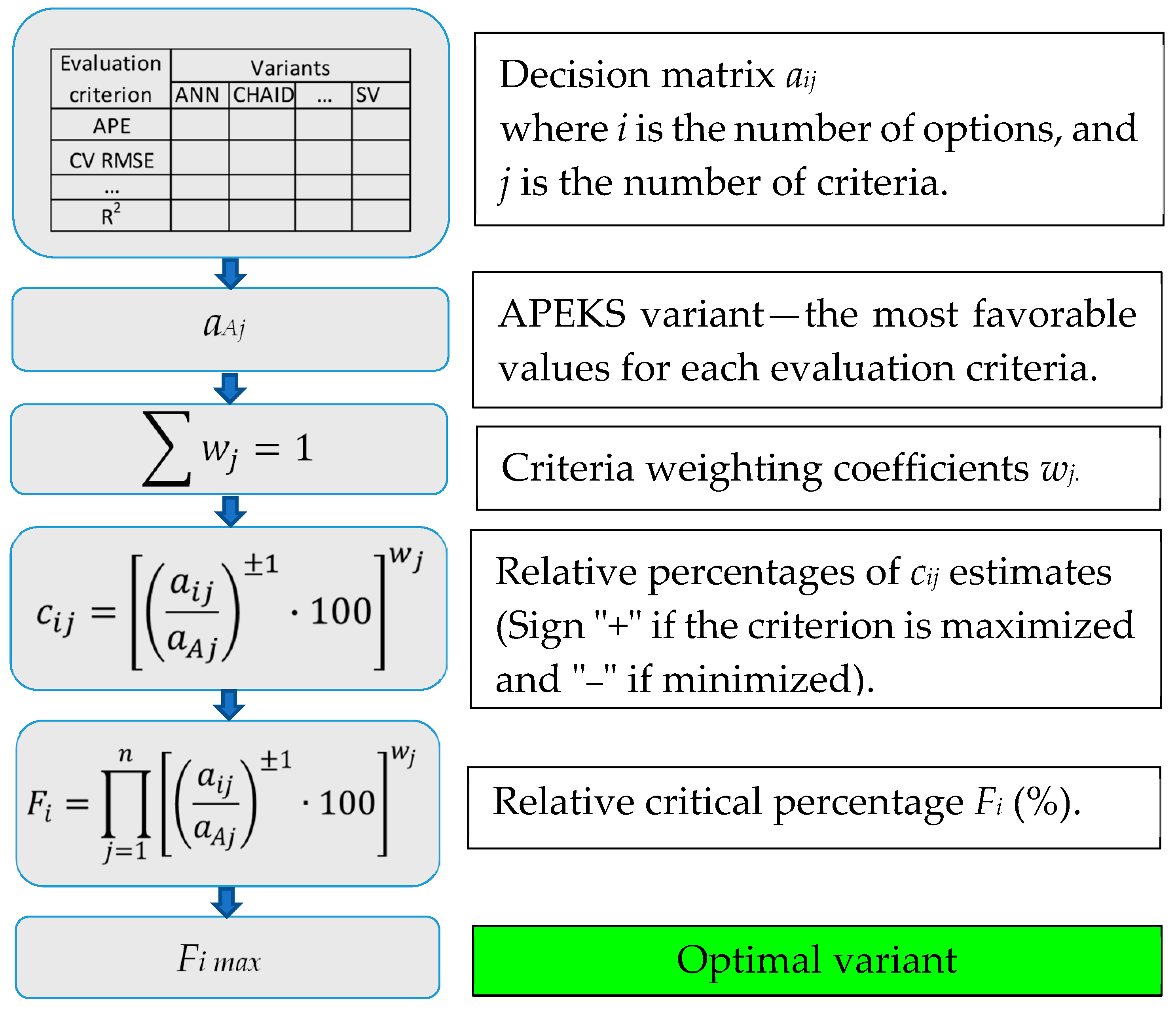
The set of indicators used in this study enables a multi-criteria approach to evaluating the forecasting models built. In the final stage of the study, the multi-criteria APEKS method [50] was used for a comprehensive evaluation that takes all criteria into account simultaneously. This method has the advantage of producing a dimensionless score, which is a percentage rating of the individual models reviewed. The model that achieved the highest score using this method is preferred. The algorithm for implementing the evaluation process is shown in Figure 1, while Figure 2 shows the algorithm for evaluating the quality of the models using the selected indicators.

4. Characteristics of the Research Object

The research material used to achieve the study’s objectives, describing 2477 municipalities in Poland, was compiled from publicly available statistical data [51] and the paper by Banski [52]. The study by Banski [52] categorizes municipalities based on three main characteristics: administrative type (C2), functional type (C3), and range of influence (C4). Within the administrative type, categories include urban, urban–rural, and rural municipalities. Functional types distinguish urban, urbanized, multifunctional transitional, overwhelmingly or prevalently agricultural, tourism and recreational, forestry, and mixed-function municipalities. Finally, the range of influence typology categorizes municipalities as the cores of urban centers, zones with the strongest actual and potential impacts (suburban zones), poorly accessible strong-impact zones, zones with weak potential impacts (external zones), and peripheral zones. A list of independent variables is presented in

Table 2. List of independent variables.

Symbol Attribute	Name of Independent Variable	Unit
C1	voivodeship	—
C2	municipality administrative type	—
C3	functional structure of communes	—
C4	typology of municipalities according to the scope of impact	—
C5	population density	per·km−2
C6	building occupancy rate	per·apartment−1
C7	average agricultural area	ha
C8	percentage of apartments heated with natural gas	%
C9	average gas consumption for residential heating by household	MWh·apartment−1
C10	share of apartments equipped with water supply	%
C11	share of apartments equipped with sewage systems	%
C12	share of apartments equipped with a gas installation	%
C13	share of apartments equipped with a flush toilet	%
C14	share of apartments equipped with a bathroom	%
C15	share of farms deriving income from agricultural activities	%
C16	personal income tax	PLN·per−1
C17	corporate income tax	PLN·per−1
C18	municipal waste management expenses	PLN·per−1
C19	feminization ratio (number of women per 100 men)	person
C20	persons of non-working age per 100 persons of working age	person
C21	persons of post-working age per 100 persons of pre-working age	person
C22	persons of post-working age per 100 persons of working age	person
C23	migration balance per 1000 population	person
C24	indicator of enterprises carrying out collection of mixed municipal waste	%
C25	rate of provision of municipal waste collection services from residential properties	%
C26	rate of provision of municipal waste collection services from unoccupied properties	%
C 27	cost efficiency ratio of total services of municipal waste collected	PLN·Mg−1
C28	total registered unemployed in population	%
C29	number of apartments in the building	pcs
C30	number of live births per 1000 people	—
C31	natural increase per 1000 inhabitants	%

.

The collected dataset was subjected to pre-processing, which involved removing objects for which complete data were missing or those that were considered outliers. After confirming the assumption of the normal distribution of the data, outliers were classified as those whose values exceeded the interval of the mean value ± 3 times the standard deviation. A learning set containing 70% of the observations and a test set containing the remaining 30% of the observations were then randomly separated.

5. Research Results

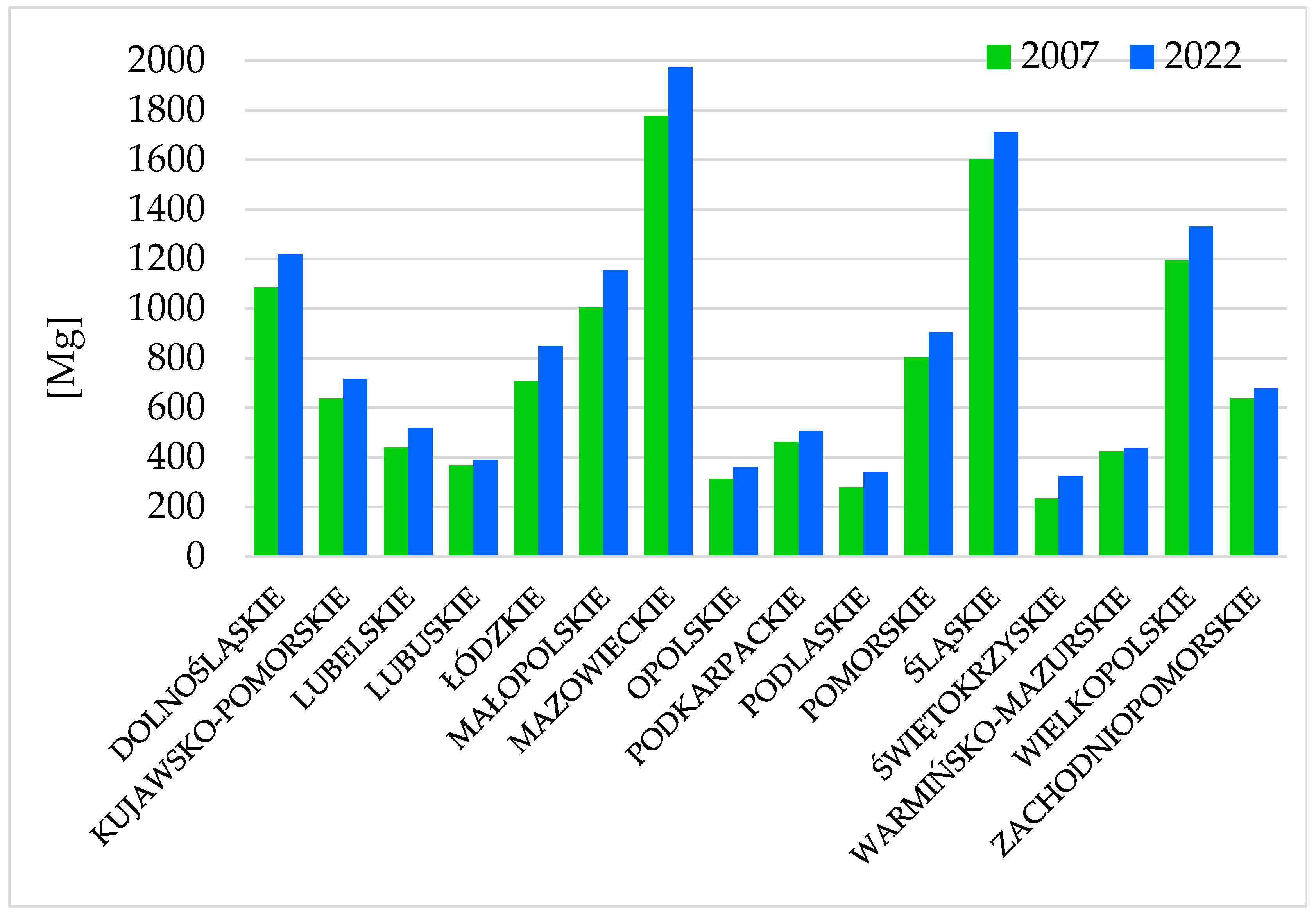
Prior to the construction of the forecasting models, an analysis of the temporal and spatial variation in the amount of municipal waste collected from the study regions was performed (Figure 3). Due to the large number of facilities, Figure 4 shows the amount of waste collected by province. The largest amounts of waste were collected in the Mazowieckie and Silesian voivodeships, with 1777 and 1601 thousand tons in 2007, and 1974 and 1713 thousand tons in 2022, respectively. There is a wide variation in the amount of municipal waste collected in Poland, but in each region, the amount is increasing over time.

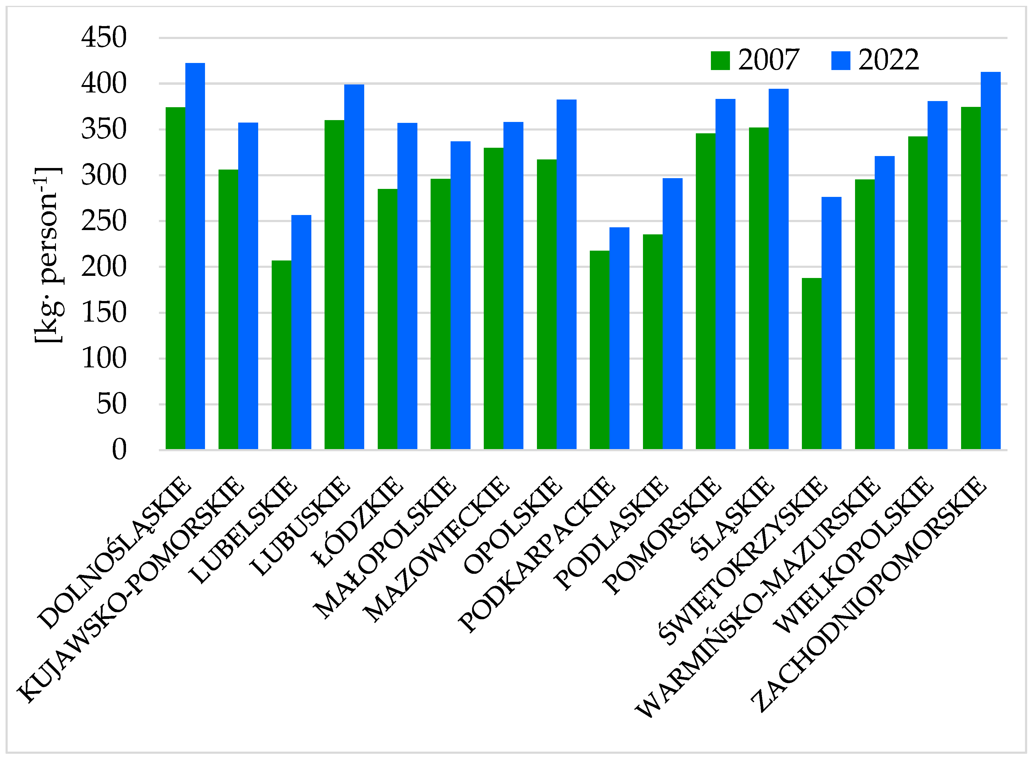
The level of the mass accumulation rate of municipal waste is influenced by many factors, both social and economic. To compare regions, per capita unit waste accumulation rates were determined. High variability was also observed in this analysis. In 2022, residents of the Lower Silesian and West Pomeranian voivodeships generated the most waste (over 400 kg·person⁻¹). In contrast, the least amount of waste (about 250 kg·person⁻¹) was collected in the Podkarpackie, Lubuskie, and Świętokrzyskie provinces.

Similarly, an increase in the amount of municipal waste generated per person was observed for the aggregate indicator. In contrast, the least amount of waste (about 250 kg·person⁻¹) was collected in the Podkarpackie, Lubuskie, and Świętokrzyskie provinces.

The largest changes over the 2007–2022 period occurred in the Świętokrzyskie (an increase of 88 kg·person⁻¹) and Łódzkie (an increase of 72 kg·person⁻¹) provinces. Even greater variation was observed at the level of municipalities, where the rate of waste accumulation, after the removal of outlier observations, oscillated from 52 kg·person⁻¹ to 662 kg·person⁻¹.

Waste collected from residents is recycled, composted, digested, thermally transformed with energy recovery, or landfilled. On average, about 22–24% of waste is thermally transformed. Due to the existing infrastructure, this rate varies from 10 to 46%.

According to current legislation and good practices, sustainable waste management should be pursued. One of the key measures is to reduce the amount of landfilled waste, including by thermally transforming fractions with energy value that are not recyclable. Achieving this goal requires significant investment in the construction of waste conversion facilities with energy recovery and a system for receiving electricity and heat.

Due to the variability of the waste stream in time and space, forecasts that allow for the technical and economic evaluation of planned investments are crucial. Reliable forecasts are one of the main determinants of development in this area.

We now have effective methods and computational tools at our disposal. The key challenge is selecting the right decision variables to develop predictions with acceptable errors over a given time horizon. Boruta algorithm [47] was used to select independent variables in predictive models. This is a recursive variable selection method based on the random forest algorithm. Its purpose is to identify independent variables that do not significantly contribute to the prediction of the dependent variable and remove them from the predictive model.

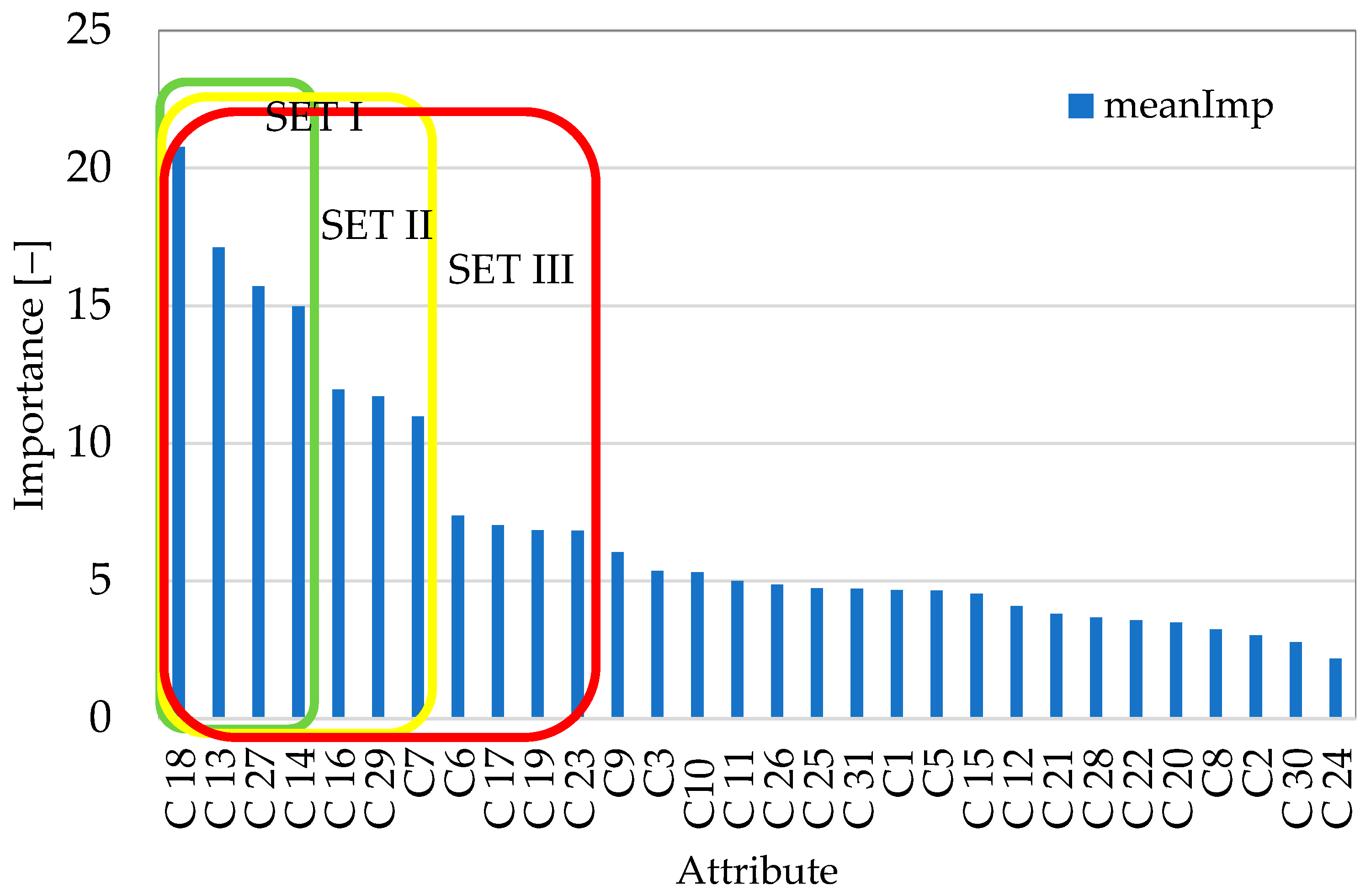
The selection process proceeds iteratively, with each iteration removing more features with the least importance. As a result, the Boruta algorithm provides a set of independent variables that are relevant to the prediction of the dependent variable and are not highly correlated with each other. In addition, a ranking of the features (attribute importance) considered most relevant to the model is produced. A detailed description of how the algorithm works is presented in a previous paper [48]. For the selection of attribute importance, the Boruta package in the R program (version R–4.4.0) was used [49]. The results of the conducted evaluation of the importance of attributes are shown in Figure 5.

Applying the Boruta algorithm, from a group of 31 conditional variables, 24 variables emerged and were ranked according to their importance. Analyzing the chart of the rankings reveals that 11 variables clearly stand out from the others (marked in red) (Figure 5). Additionally, in the analyzed group, it is possible to distinguish three sets of conditional variables with varying degrees of importance: high (C18, C13, C27, C14), medium (C16, C29, C7), and the remaining variables (C6, C17, C19, C23). With this in mind, the authors decided to create three sets that differ in the number of conditional variables. These groups were named SET I, SET II, and SET III.

SET I contained four variables: municipal waste management expenditures [PLN·person⁻¹] (C18), the share of apartments equipped with a flush toilet [%] (C13), the total cost-effectiveness ratio of municipal waste collection services [PLN·Mg⁻¹] (C27), and the share of apartments equipped with a bathroom [%] (C14).

SET II was further expanded to include three additional variables: personal income tax [PLN·person⁻¹] (C16), the number of dwellings in a building (C29), and the average area of agricultural land [ha] (C7).

SET III, the largest set, was further expanded to include four additional variables: the ratio of the number of people in a dwelling [person·apartment⁻¹] (C6), the amount of corporate income tax [PLN·person⁻¹] (C17), the feminization rate, which is the number of women per 100 men [person] (C19), and the migration balance per 1000 people [person] (C23). SET I, SET II, and SET III are circled in green, yellow, and red, respectively, in Figure 5.

The different sets of variables (SET I, SET II, and SET III) were input into the selected predictive models, and the results obtained on the test set were evaluated for quality and accuracy using eight evaluation metrics: CV RMSE, MAE, MAPE, MBE, ME, MPE, PE, and R².

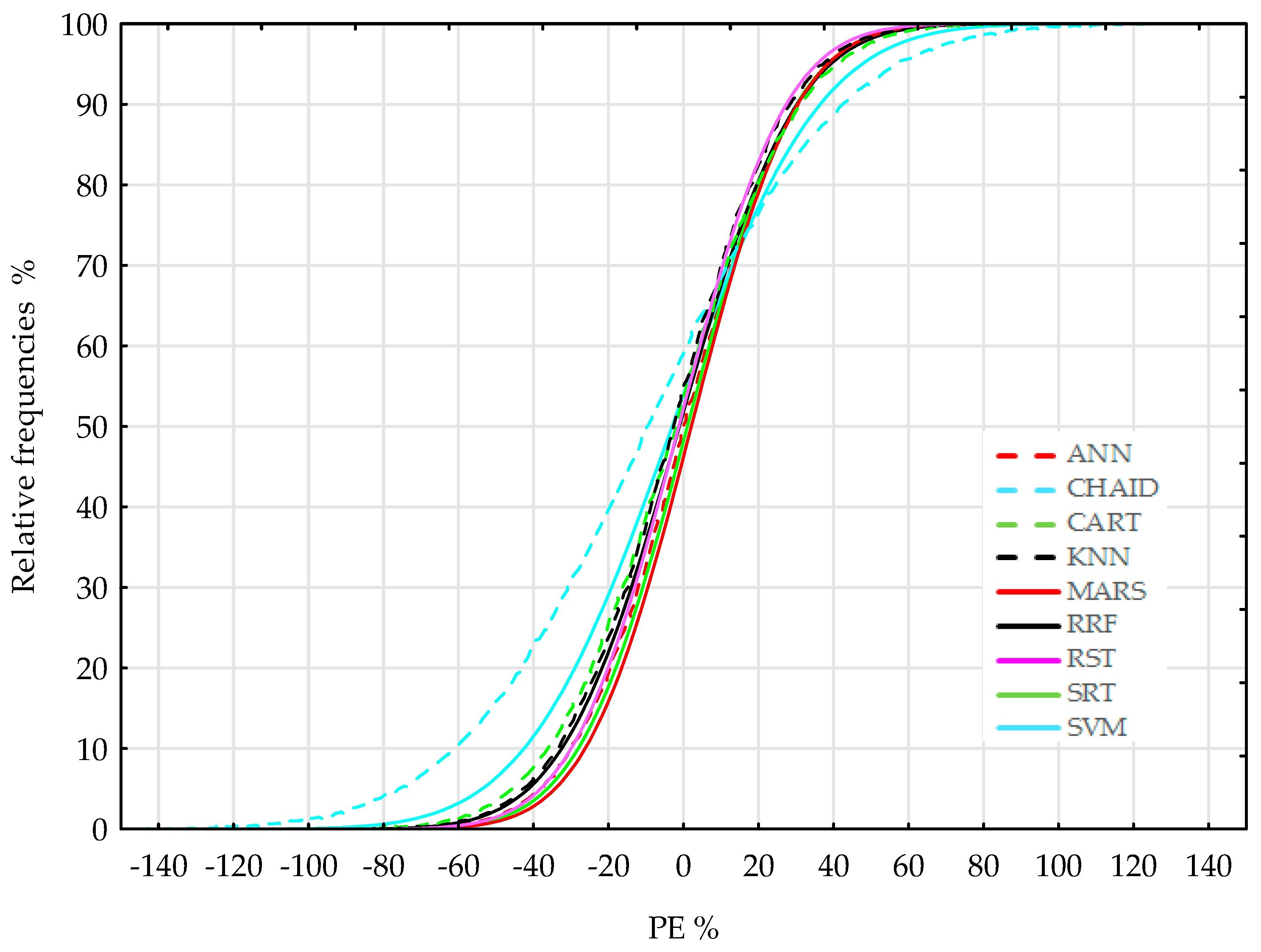
The error values for each set are summarized in

Table 3. Evaluation of the quality of SET I models.

4 Variables	ANN	CHAID	CART	KNN	MARS	RRF	RST	SRT	SVM
CVRMSE	20.1	30.7	22.8	21	20.9	21.2	20	21.7	26.9
MAE	37.4	63.8	46.2	43.2	40.4	42.7	38.8	42.1	52.4
MAPE	14.7	28.1	18.9	17.9	15.6	17.4	15.4	16.5	21.9
MBE	5.1	2.1	3.8	4.6	6.8	4.0	1.3	6.3	4.6
ME	13.6	5	9.9	12.3	18.1	10.4	3.5	16.8	12.1
MPE	0.3	−9.4	−2.4	−1.1	2.1	−2.7	−1.3	1	−3.1
R2	0.77	0.41	0.69	0.74	0.76	0.76	0.76	0.74	0.56

,

Table 4. Evaluation of the quality of SET II models.

7 Variables	ANN	CHAID	CART	KNN	MARS	RRF	RST	SRT	SVM
CVRMSE	30.6	33.2	30.4	27.4	26.1	28.5	18.8	25.9	25.3
MAE	48.9	53.4	48.8	41.4	31.2	43	37.6	35.3	49
MAPE	19.4	20.7	19.3	16.2	11.8	17.2	14.8	13.8	20.5
MBE	3.8	3.9	1.7	3.6	2.1	2.4	1.8	1.4	3.1
ME	10.2	10.6	4.6	9.6	5.6	6.6	4.8	3.8	8.4
MPE	−2	−3.4	−4.6	−1.5	−0.9	−4.3	−0.7	−2.4	−3.7
R2	0.56	0.48	0.56	0.65	0.68	0.63	0.78	0.68	0.71

and

Table 5. Evaluation of the quality of SET III models.

11 Variables	ANN	CHAID	CART	KNN	MARS	RRF	RST	SRT	SVM
CVRMSE	19.2	26.3	21.4	20.2	19.1	20.4	19.6	16.5	21.5
MAE	38.2	54.8	42.6	41.3	29.4	41.3	38.3	32.8	44.6
MAPE	15.4	24.3	17.6	16.9	11.7	17.6	14.8	13.5	18.7
MBE	4.1	0.2	0.9	3.4	1.3	1.2	2.9	0.6	2.5
ME	10.9	0.6	2.5	9	3.5	3.2	7.7	1.6	6.8
MPE	−0.9	−7.9	−4.1	−1.4	−0.9	−5.2	0.4	−2.7	−3.1
R2	0.79	0.57	0.72	0.76	0.78	0.76	0.77	0.83	0.72

and Figure 6, Figure 7 and Figure 8. When analyzing the quality evaluation metrics of the developed models for the first set of variables (C18, C13, C27, and C14), the best method in terms of all evaluation metrics was not identified. The ANN method proved to be the best in terms of the MAE, MAPE, MBE, and coefficient of determination. It had a slight advantage over the RST method, which additionally had the lowest CV RMSE, MBE, and ME values. The MARS method also exhibited low error values. However, in terms of ME, it was significantly worse compared to RST. The average error of 18 kg·person⁻¹ indicates that this method tends to underestimate municipal waste accumulation rates. Since the indicators presented in Table 3 mostly show only the average values, this paper also develops error distributions to assess the proportion of observations of a given quality.

Figure 6 shows the course of each model’s residual distribution in relative form with its sign. This makes it possible to assess quality separately in terms of overprediction and underprediction.

This study identified two methods characterized by different PE error distributions: the support vector (SVM) method and the exhaustive regression tree (CHAID) method. For these methods, the proportion of forecasts underestimated by more than 40% was 12% and 7%, respectively, while for the other methods, it was below 5%. Even larger errors were observed in relation to the overestimation of forecasts. The share of errors with values greater than 40% for the CHAID method was as high as 23%, and for SVM, it was 11%. Information on the trend of a forecasting method in terms of overestimation and underestimation is very valuable if different operating costs are caused by over- or underprediction.

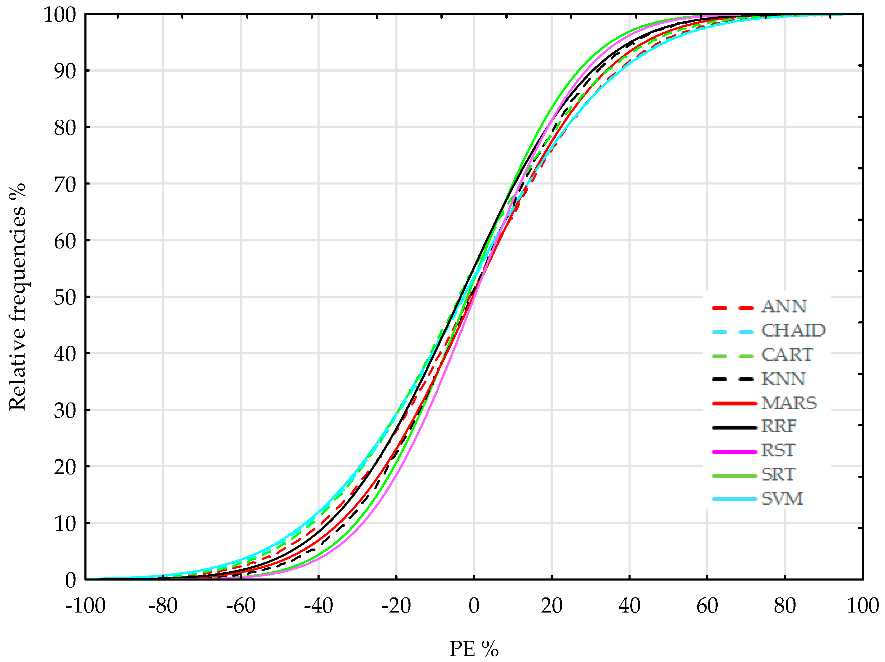
Using the variables of SET II (C18, C13, C27, C14, C16, C29, C7), it was observed (Table 4) that rough sets (RST) and support regression trees (SRTs) were superior to the other methods. The former method has the lowest CVRMSE, MPE, and R² error. In contrast, boosted regression trees make it possible to make predictions with lower MAE, MBE, and ME. The MARS method should also be of interest in waste stream forecasting. It is the best in terms of MAE and MAPE. The differences between the methods are insignificant, amounting to about 2%.

Also, in Figure 7, which shows the course of the empirical distributions of the PE error, variation among the compared methods is not apparent. Similar to SET I, the largest share of errors with values exceeding ±40% was observed for the support vector method and the advanced regression tree (CHAID) method. An increase in the share of errors with large values was also observed for the ANN method and the CART advanced regression tree method. The former method was characterized by an increase in errors resulting from underprediction, and the latter, on the contrary, from overprediction. The highest frequency of errors with the lowest values was observed for the enhanced regression tree method and methods using rough set theory.

The introduction of additional independent variables (C16, C29, C7) resulted in a deterioration in the quality of predictions assessed by the CVRMSE index for most cases, except for RST and SVM (Table 4). The increase in error values ranged from 2.5% for CHAID to more than 10% for ANN. A similar trend was also observed for the MPE, which also increased for most methods. For the remaining indicators, the introduction of more independent variables had the desired effect. However, when comparing the best methods from SET I to SET II, the CVRMSE, MAE, and MAPE quality indexes improved by 1.2%, 6.2 kg·person⁻¹, and 2.9%, respectively. Introducing more variables into the models’ inputs for the other indicators did not result in an improvement in quality but in a deterioration. However, these were changes on the order of 1% for MPE and even smaller for the others.

The next sample used the third set of variables, SET III, with the largest number of independent variables. It used variables from the first set, SET I, and the second set, SET II, which were additionally supplemented by variables C6, C17, C19, and C23. For the most extensive set of variables, a further increase in the variation of method quality was observed according to the evaluation criteria (Table 5).

In SET I, the best indicators narrowed the choice down to only two methods, namely, ANNs and RST. In SET II, the best method had to be sought among three methods (RST, SRT, and MARS). In the next set, SET III, the best quality indicators were spread among four methods, namely, CHAID, MARS, RST, and SRTs. Each of these methods exhibited the best quality, but only in terms of one or two evaluation indicators.

The CHAID method produced the best predictions in terms of the MBE and ME. Unfortunately, this method has twice the MAE and MAPE values compared to the MARS method. Between the MARS, RST, and SRT methods, there was no longer as much variation, but it is still impossible to clearly identify and select the preferred method. Analyzing the error values summarized in Table 5, one can detect a slight advantage of the MARS method over the other methods. It has an almost 3% higher CVRMSE value than SRTs, but the absolute error values of MAE and relative error values of MAPE indicate its superiority over the others.

The developed PE error distributions for each method confirm that the RST and SRT methods have the highest proportion of errors that are at the low end (Figure 8). The advantage of rough set theory over the other methods is particularly evident for overestimated forecasts. Similarly, as for the other sets of variables, the highest number of forecasts with high errors was registered for the support vector method. This method generated forecasts in which almost 20% of observations were overestimated by more than 40% and less than 10% underestimated at this level.

The performed comparative analysis of the selected methods used to forecast the stream of municipal waste accumulation collected from households in municipalities did not clearly indicate any method as superior.

To make a comprehensive assessment considering all analyzed quality assessment criteria, a comparison of models was made using the APEKS method. This is a multi-criteria method, and its course of action is shown in the methodology in Figure 3. During the study, all criteria were compared with each other for the APEKS variant that had the best features among the analyzed variants. The method provided an opportunity to vary the importance of the evaluation criteria by assigning weights to them, for example, using the normalized von Neumann–Morgenstern gambling method [54] or the Achoff–Churchman method [55].

Since the purpose of this work did not clearly indicate the preferred criteria for assessing the quality of the models built, it was decided not to differentiate them by weights. The best predictive model is the one for which the relative critical percentages Fi take the highest value.

Table 6. Relative percentages of Fi critical values of the studied forecast models.

Relative Critical Percentages	Types of Forecasting Models
	ANN	CHAID	CART	KNN	MARS	RRF	RST	SRT	SVM
Fi (%) SET I	68	39	50	54	46	50	80	51	41
Fi (%) SET II	50	44	56	58	81	55	88	75	51
Fi (%) SET III	34	48	40	33	51	36	43	55	31

where: green indicates the best and red the worst models, taking into account all their evaluation indicators according to the APEKS method.

shows the obtained critical values for individual methods and sets of independent variables, where the green color indicates the best method, while the red color indicates the least effective method.

For SET I, containing the smallest number of independent variables, the RST method was considered the best when considering all evaluation criteria. The value of the summary evaluation index Fi was 80%. The second-best method was the ANN (artificial neural network) method, scoring 68%. CHAID and SVM were rated the lowest, scoring 39% and 41%, respectively.

In SET II, the method using rough set theory and the MARS method can be considered preferred, characterized by Fi evaluation rates of 88% and 81%, respectively. The next method in the ranking is SRTs, with a rating of 75%. CHAID, SVM, and ANNs were still rated the lowest, with ANNs being considered the alternative preferred method for SET I.

For the broadest set of input variables, SET III, there was less variation among the evaluated methods. The CHAID, MARS, and SRT methods were considered the most effective, with Fi rates between 48% and 55%. However, their advantage over the others was only a few percent. The lowest rating, just over 30%, was given to KNN and SVM.

Since the evaluation was conducted for the APEKS variant, which exhibits the best features among the analyzed variants, a combined analysis for all methods and sets of variables was conducted. This evaluation identified the method and variant with the best quality for the adopted evaluation criteria. The results of the analysis are summarized in

Table 7. Relative critical Fi percentages of the tested models and sets of variables.

	SET III	SET III	SET III	SET II	SET I	SET II
Relative critical percentages	SRT	MARS	CHAID	RST	RST	MARS
Fi (%)	52.36	49.36	45.80	43.68	42.84	40.03

.

Of the variants studied, SRTs, CHAID, and MARS were considered the preferred methods, for which the independent variables were the conditional variables with the highest degree of importance, labeled as C18, C13, C27, C14, C16, C29, C7, C6, C17, C19, and C23.

If, due to workload or a lack of access to information, the set with the least number of variables (C18, C13, C27, C14) is used, then the rough set method should be used to develop the forecast. The use of an intermediate set is not advisable, as it does not guarantee an improvement in the quality of the forecast relative to a set with fewer variables, but only forces the collection of more independent variables.

6. Results and Discussion

Based on a survey of 2477 municipalities in Poland, 31 potential independent variables representing the municipal waste accumulation rate were pre-selected. The application of the Boruta algorithm allowed the assessment of the importance of these variables. This information was used to create three sets of independent variables with different sizes: 4 variables—C18, C13, C27, and C14; 7 variables—C18, C13, C27, C14, C16, C29, and C7; and 11 variables—C18, C13, C27, C14, C16, C29, C7, C6, C17, C19, and C23.

The first set, SET I (four variables), included two social variables representing the standard of living of residents and two economic variables on municipal waste management expenditures. SET II (seven variables) was supplemented by two social variables (the number of dwellings in a building and the average area of agricultural land) and one economic variable representing the average personal income tax rate. SET III (eleven variables) included seven social variables (expanded to encompass the average number of people per housing unit, feminization rate, and migration balance) and four economic variables (supplemented by corporate income tax).

The variables grouped into each set were used to build forecasting models using the selected methods, namely, ANNs, CHAID, CART, KNN, MARS, RRFs, RST, SRTs, and SVM. The study indicates that, for the set with the smallest number of variables but the highest degree of importance (SET I), the RST method is preferred due to its forecast quality. It generates forecasts with a MAPE of 15% and an R² of 0.76. With a comprehensive evaluation by the APEKS method, considering all criteria, it obtains a relative percentage of 80%. The second method, with a critical value of 68%, is the ANN method.

SET II, the second set, which also includes variables of medium importance, had similar error rates. No significant improvement in model quality was observed for the SET I set of variables either. The best forecasts were obtained for RST and MARS.

A reduction in forecast error was observed for the largest set of variables (SET III). The MAPE for most methods oscillated between 11.7% for MARS and 17.6% for CART. The exception was the CHAID method, for which the rate was 24.3%. The coefficient of determination R² was between 0.72 for CART and 0.83 for RST. As before, the lowest R² score (0.57) was obtained by the CHAID method. Using selected variables from SET III to develop a model using the SRT, CHAID, or MARS methods produced the best predictions while considering all evaluation indicators. These methods are preferred if we have access to the group of independent variables that constitute SET III. In the case of limited access to data (SET I), the RST and ANN methods should be preferred. The use of an intermediate set between SET I and SET III is not advisable, as it increases the effort to collect data and does not improve the quality of the forecast.

In the literature, there are mostly reports comparing two methods, for example, the effectiveness of artificial neural networks and multiple linear regression [29], artificial neural network and support vector machine techniques [39], regression and trend analysis [40], support vector machines and hybrids of wavelet transform–support vector machine models [41], a Long Short-Term Memory (LSTM) neural network and ARIMA [42], and Multi-Linear Regression (MLR) and Gradient Boosting Regression Tree (GBRT) [43]. Unfortunately, these works do not consider the impact of the deliberate selection of the set of independent variables for each method on the quality of the obtained forecasts. The models presented in this paper for forecasting the municipal waste accumulation rate are of better quality than most of those reported in the literature. The R² coefficients of determination obtained in this study were at the level of 0.76–0.78, while those in other studies oscillate between 0.42 and 0.86. Additionally, the MAPE index was at a low level, ranging between 13.5 and 14.8%. There are examples in the literature of models with much lower errors (8–9% [39], R² = 0.97 [44]), but it is difficult to refer to the conditions under which these studies were carried out. Furthermore, choosing the preferred method often involves a compromise between the quality of the forecast and the required amount of information for the independent variables.

Future studies will be conducted on groups of sites in different regions of the world. This study will make it possible to verify the effectiveness of the selection of variables and the choice of the preferred method or group of methods. Efforts will also be made to build hybrid models combining the best methods in terms of the evaluation criteria adopted.

References

1. Famielec, S.; Malinowski, M.; Tomaszek, K.; Wolny-Koładka, K.; Krilek, J. The effect of biological methods for MSW treatment on the physicochemical, microbiological and phytotoxic properties of used biofilter bed media. Waste Manag. 2024, 175, 276–285. [Google Scholar] [CrossRef] [PubMed]
2. Izquierdo-Horna, L.; Kahhat, R.; Vázquez-Rowe, I. Reviewing the influence of sociocultural, environmental and economic variables to forecast municipal solid waste (MSW) generation. Sustain. Prod. Consum. 2022, 33, 809–819. [Google Scholar] [CrossRef]
3. Abdallah, M.; Abu Talib, M.; Feroz, S.; Nasir, Q.; Abdalla, H.; Mahfood, B. Artificial intelligence applications in solid waste management: A systematic research review. Waste Manag. 2020, 109, 231–246. [Google Scholar] [CrossRef] [PubMed]
4. Klimek, P. Ocena potencjału energetycznego odpadów komunalnych w zależności od zastosowanej technologii ich utylizacji. Nafta-Gaz 2013, 12, 909–914. Available online: http://www.archiwum.inig.pl/INST/nafta-gaz/nafta-gaz/Nafta-Gaz-2013-12-05.pdf (accessed on 6 March 2024). (In Polish).
5. Wielgosinski, G. Wybór technologii termicznego przekształcania odpadów komunalnych. Nowa Energ. 2012, 1, 66–80. Available online: https://scholar.google.com/scholar_lookup?title=Wyb%C3%B3r+technologii+termicznego+przekszta%C5%82cania+odpad%C3%B3w+komunalnych&author=Wielgosinski,+G.&publication_year=2012&journal=Nowa+Energ.&volume=1&pages=66%E2%80%9380 (accessed on 1 April 2024). (In Polish).
6. de Morais Vieira, V.H.A.; Matheus, D.R. The impact of socioeconomic factors on municipal solid waste generation in São Paulo, Brazil. Waste Manag. Res. 2018, 36, 79–85. [Google Scholar] [CrossRef] [PubMed]
7. Abbasi, M.; Hanandeh, A.E. Forecasting municipal solid waste generation using artificial intelligence modelling approaches. Waste Manag. 2016, 56, 13–22. [Google Scholar] [CrossRef]
8. Khan, A.H.; López-Maldonado, E.A.; Khan, N.A.; Villarreal-Gómez, L.J.; Faris, M.; Munshi, F.M.; Alsabhan, A.H.; Kahkashan Perveen, K. Current solid waste management strategies and energy recovery in developing countries—State of art review. Chemosphere 2022, 291, 133088. [Google Scholar] [CrossRef]
9. Przydatek, G. Recognition of systemic differences in municipal waste management in selected cities in Poland and the United States. Environ. Sci. Pollut. Res. 2023, 30, 76217–76226. [Google Scholar] [CrossRef]
10. Nęcka, K.; Szul, T.; Knaga, J. Identification and Analysis of Sets Variables for of Municipal Waste Management Modelling. Geosciences 2019, 9, 458. [Google Scholar] [CrossRef]
11. Kundariya, N.; Mohanty, S.S.; Varjani, S.; Hao Ngo, H.; Wong, J.W.C.; Taherzadeh, M.J.; Chang, J.-S.; Yong Ng, H.; Kim, S.-H.; Bui, X.-T. A review on integrated approaches for municipal solid waste for environmental and economical relevance: Monitoring tools, technologies, and strategic innovations. Bioresour. Technol. 2021, 342, 125982. [Google Scholar] [CrossRef] [PubMed]
12. Sinha, R.; Prabhudev, B.C. Impact of socio-cultural challenges in solid waste management. Int. J. Eng. Res. Technol. (IJERT) 2016, 4, 1–3. Available online: https://www.ijert.org/research/impact-of-socio-cultural-challenges-in-solid-waste-management-IJERTCONV4IS27036.pdf (accessed on 10 April 2024).
13. Lebersorger, S.; Beigl, P. Municipal solid waste generation in municipalities: Quantifying impacts of household structure, commercial waste and domestic fuel. Waste Manag. 2011, 31, 1907–1915. [Google Scholar] [CrossRef]
14. Trang, P.T.T.; Dong, H.Q.; Toan, D.Q.; Hanh, N.T.X.; Thu, N.T. The Effects of Socio-economic Factors on Household Solid Waste Generation and Composition: A Case Study in Thu Dau Mot, Vietnam. Energy Procedia 2017, 107, 253–258. [Google Scholar] [CrossRef]
15. Ali Abdoli, M.; Falah Nezhad, M.; Salehi Sede, R.; Behboudian, S. Longterm forecasting of solid waste generation by the artificial neural networks. Environ. Prog. Sustain. Energy 2012, 31, 628–636. [Google Scholar] [CrossRef]
16. Namlis, K.G.; Komilis, D. Influence of four socioeconomic indices and the impact of economic crisis on solid waste generation in Europe. Waste Manag. 2019, 89, 190–200. [Google Scholar] [CrossRef] [PubMed]
17. Abbasi, M.; Rastgoo, M.N.; Nakisa, B. Monthly and seasonal modeling of municipal waste generation using radial basis function neural network. Environ. Prog. Sustain. Energy 2018, 38, e13033. [Google Scholar] [CrossRef]
18. Johnson, N.E.; Ianiuk, O.; Cazap, D.; Liu, L.; Starobin, D.; Dobler, G.; Ghandehari, M. Patterns of waste generation: A gradient boosting model for short-term waste prediction in New York City. Waste Manag. 2017, 62, 3–11. [Google Scholar] [CrossRef]
19. Shah, A.V.; Srivastava, V.K.; Mohanty, S.S.; Varjani, S. Municipal solid waste as a sustainable resource for energy production: State-of-the-art review. J. Environ. Chem. Eng. 2021, 9, 105717. [Google Scholar] [CrossRef]
20. Han, Z.; Liu, Y.; Zhong, M.; Shi, G.; Li, Q.; Zeng, D.; Zhang, Y.; Fei, Y.; Xie, Y. Influencing factors of domestic waste characteristics in rural areas of developing countries. Waste Manag. 2018, 72, 45–54. [Google Scholar] [CrossRef]
21. Vu, H.L.; Ng, K.T.W.; Bolingbroke, D. Time-lagged effects of weekly climatic and socio-economic factors on ANN municipal yard waste prediction models. Waste Manag. 2019, 84, 129–140. [Google Scholar] [CrossRef] [PubMed]
22. Cárdenas-Mamani, Ú.; Kahhat, R.; Vázquez-Rowe, I. District-level analysis for household-related energy consumption and greenhouse gas emissions: A case study in Lima, Peru. Sustain. Cities Soc. 2022, 77, 103572. [Google Scholar] [CrossRef]
23. Giampietro, M.; Mayumi, K.; Sorman, A. The Metabolic Pattern of Societies: Where Economists Fall Short, 1st ed.; Routledge: London, UK, 2012. [Google Scholar] [CrossRef]
24. Kaza, S.; Yao, L.; Bhada-Tata, P.; Van Woerden, F. What a Waste 2.0: A Global Snapshot of Solid Waste Management to 2050; World Bank Publications: Washington, DC, USA, 2018; Available online: https://books.google.pl/books?hl=pl&lr=&id=bnN_DwAAQBAJ&oi=fnd&pg=PP13&ots=faNcyx50M8&sig=f_x48AAFyWRJScWTxyOsZxwEIsI&redir_esc=y#v=onepage&q&f=false (accessed on 11 April 2024).
25. de Souza Melaré, V.A.; Montenegro González, S.; Faceli, K.; Casadei, V. Technologies and decision support systems to aid solid-waste management: A systematic review. Waste Manag. 2017, 59, 567–584. [Google Scholar] [CrossRef] [PubMed]
26. Chhay, L.; Reyad, M.A.H.; Suy, R.; Islam, M.R.; Mian, M.M. Municipal solid waste generation in China: Influencing factor analysis and multi-model forecasting. J. Mater. Cycles Waste Manag. 2018, 20, 1761–1770. [Google Scholar] [CrossRef]
27. Nguyen, X.C.H.; Nguyen, T.T.H.; La, D.D.; Kumar, G.; Rene, E.R.; Nguyen, D.D.; Chang, S.W.; Chung, W.J.; Nguyen, X.H.; Nguyen, V.K. Development of machine learning—Based models to forecast solid waste generation in residential areas: A case study from Vietnam. Conserv. Recycl. 2021, 167, 105381. [Google Scholar] [CrossRef]
28. Popli, K.; Park, C.; Han, S.-M.; Kim, S. Prediction of Solid Waste Generation Rates in Urban Region of Laos Using Socio-Demographic and Economic Parameters with a Multi Linear Regression Approach. Sustainability 2021, 13, 3038. [Google Scholar] [CrossRef]
29. Azadi, S.; Karimi-Jashni, A. Verifying the performance of artificial neural network and multiple linear regression in predicting the mean seasonal municipal solid waste generation rate: A case study of Fars province, Iran. Waste Manag. 2016, 48, 14–23. [Google Scholar] [CrossRef] [PubMed]
30. Sunayana; Kumar, S.; Kumar, R. Forecasting of municipal solid waste generation using non-linear autoregressive (NAR) neural models. Waste Manag. 2021, 121, 206–214. [Google Scholar] [CrossRef] [PubMed]
31. Guyon, I.; Elisseeff, A. An introduction to variable and feature selection. J. Mach. Learn. Res. 2003, 3, 1157–1182. Available online: https://www.jmlr.org/papers/volume3/guyon03a/guyon03a.pdf?ref=driverlayer.com/web (accessed on 11 April 2024).
32. Lin, K.; Zhao, Y.; Kuo, J.-H.; Deng, H.; Cui, F.; Zhang, Z.; Zhang, M.; Zhao, C.; Gao, X.; Zhou, T.; et al. Toward smarter management and recovery of municipal solid waste: A critical review on deep learning approaches. J. Clean. Prod. 2022, 346, 130943. [Google Scholar] [CrossRef]
33. Orsoni, A.; Karadimas, N.V.; Loumos, V. Municipal Solid Waste Generation Modelling Based on Fuzzy Logic; European Council for Modeling and Simulation ECMS: Caserta, Italy, 2006; pp. 309–314. [Google Scholar] [CrossRef]
34. Szul, T.; Nęcka, K.; Lis, S. Application of the Takagi-Sugeno Fuzzy Modeling to Forecast Energy Efficiency in Real Buildings Undergoing Thermal Improvement. Energies 2021, 14, 1920. [Google Scholar] [CrossRef]
35. Chen, H.W.; Chang, N.-B. Prediction analysis of solid waste generation based on grey fuzzy dynamic modeling. Resour. Conserv. Recycl. 2000, 29, 1–18. [Google Scholar] [CrossRef]
36. Intharathirat, R.; Salam, P.A.; Kumar, S.; Untong, A. Forecasting of municipal solid waste quantity in a developing country using multivariate grey models. Waste Manag. 2015, 39, 3–14. [Google Scholar] [CrossRef] [PubMed]
37. Mwenda, A.; Kuznetsov, D.; Mirau, S. Time series forecasting of solid waste generation in Arusha city-Tanzania. Math. Theory Model. 2014, 4, 29–39. Available online: https://core.ac.uk/download/pdf/234679771.pdf (accessed on 15 April 2024).
38. Owusu-Sekyere, E.; Harris, E.; Bonyah, E. Forecasting and Planning for Solid Waste Generation in the Kumasi Metropolitan Area of Ghana: An ARIMA Time Series Approach. Int. J. Sci. 2013, 2, 69–83. [Google Scholar] [CrossRef]
39. Ayeleru, O.O.; Fajimi, L.I.; Oboirien, B.O.; Olubambi, P.A. Forecasting municipal solid waste quantity using artificial neural network and supported vector machine techniques: A case study of Johannesburg, South Africa. J. Clean. Prod. 2021, 289, 125671. [Google Scholar] [CrossRef]
40. Ghinea, C.; Drăgoi, E.N.; Comăniţă, E.-D.; Gavrilescu, M.; Câmpean, T.; Curteanu, S.; Gavrilescu, M. Forecasting municipal solid waste generation using prognostic tools and regression analysis. J. Environ. Manag. 2016, 182, 80–93. [Google Scholar] [CrossRef] [PubMed]
41. Abbasi, M.; Abduli, M.A.; Omidvar, B.; Baghvand, A. Results uncertainty of support vector machine and hybrid of wavelet transform-support vector machine models for solid waste generation forecasting. Environ. Prog. Sustain. Energy 2014, 33, 220–228. [Google Scholar] [CrossRef]
42. Cubillos, M. Multi-site household waste generation forecasting using a deep learning approach. Waste Manag. 2020, 115, 8–14. [Google Scholar] [CrossRef]
43. Shuyan Wan, S.; Nik-Bakht, M.; Tsun Wai Ng, K.; Tian, X.; An, C.; Sun, H.; Yue, R. Insights into the urban municipal solid waste generation during the COVID-19 pandemic from machine learning analysis. Sustain. Cities Soc. 2024, 100, 105044. [Google Scholar] [CrossRef]
44. Younes, M.K.; Nopiah, Z.M.; Basri, N.E.A.; Basri, H.; Maulud, K.N.A. Prediction of municipal solid waste generation using nonlinear autoregressive network. Environ. Monit. Assess. 2015, 187, 753. [Google Scholar] [CrossRef] [PubMed]
45. Xu, A.; Chang, H.; Xu, Y.; Li, R.; Li, X.; Zhao, Y. Applying artificial neural networks (ANNs) to solve solid waste-related issues: A critical review. Waste Manag. 2021, 124, 385–402. [Google Scholar] [CrossRef] [PubMed]
46. Dyson, B.; Chang, N.-B. Forecasting municipal solid waste generation in a fast-growing urban region with system dynamics modeling. Waste Manag. 2005, 25, 669–679. [Google Scholar] [CrossRef] [PubMed]
47. Kursa, M.B.; Rudnicki, W.R. Wybór funkcji z pakietem Boruta. J. Stat. Oprogramowanie 2010, 36, 1–13. [Google Scholar] [CrossRef]
48. efg’s R Notes: Boruta Package. 2015. Available online: https://earlglynn.github.io/RNotes/package/Boruta/index.html (accessed on 2 May 2024). (In Polish).
49. The R Project for Statistical Computing. Available online: https://cloud.r-project.org. (accessed on 2 April 2024).
50. Szybka, J.; Pabian, S. APEKS—A method of decision making. Sci. Technol. Innov. 2021, 12, 45–50. [Google Scholar] [CrossRef]
51. Statistics Poland. Central Statistical Office. Local Data Bank. 2024. Available online: https://bdl.stat.gov.pl/.BDL/start (accessed on 15 March 2024).
52. Bański, J. Contemporary typologies of rural areas in Poland—An overview of methodological approaches. Przegląd Geogr. 2014, 86, 441–470. Available online: http://www.rcin.org.pl/Content/51257/WA51_70537_r2014-t86-z4_Przeg-Geogr-Banski.pdf (accessed on 15 March 2024). (In Polish). [CrossRef]
53. Ruiz, G.R.; Bandera, C.R. Validation of Calibrated Energy Models: Common Errors. Energies 2017, 10, 1587. [Google Scholar] [CrossRef]
54. von Neumann, J.; Morgenstern, O. Theory of Games and Economic Behavior; Princeton University Press: Princeton, NJ, USA, 1947. [Google Scholar]
55. Churchman, C.W.; Ackoff, R.L.; Arnoff, E.L. Introduction to Operations Research; Wiley: New York, NY, USA, 1957. [Google Scholar]
Figure 1. The algorithm for building forecasting models.
Energies 17 03524 g001
Figure 2. The algorithm for assessing the quality of models with selected indicators.
Energies 17 03524 g002
Figure 3. The amount of municipal waste collected in 2007 and 2022.
Energies 17 03524 g003
Figure 4. Municipal waste unit generation rates in 2007 and 2022.
Energies 17 03524 g004
Figure 5. Feature importance ranking.
Energies 17 03524 g005
Figure 6. PE error distributions for SET I.
Energies 17 03524 g006
Figure 7. PE error distributions for SET II.
Energies 17 03524 g007
Figure 8. PE error distributions for SET III.
Energies 17 03524 g008