Bus Basis Model Applied to the Chilean Power System: A Detailed Look at Chilean Electric Demand

Abstract

This paper presents a methodology to forecast electrical demand for the Chilean Electrical Power System considering a national, regional, district and bus spatial disaggregation. The methodology developed was based on different kinds of econometric models and end-use models to represent the massification of low carbon emission technologies such as electromobility, electric heating, electric water heating, and distributed generation. In addition, the methodology developed allows for the projection of the electric demand considering different kinds of clients as regulated and non-regulated clients, and different economic sectors. The model was applied to forecast the long-term electricity demand in Chile for the period 2022–2042 for 207 districts and 474 buses. The results include projections under the base case and low carbon scenarios, highlighting the significant influence of new technologies on future demand.

1. Introduction

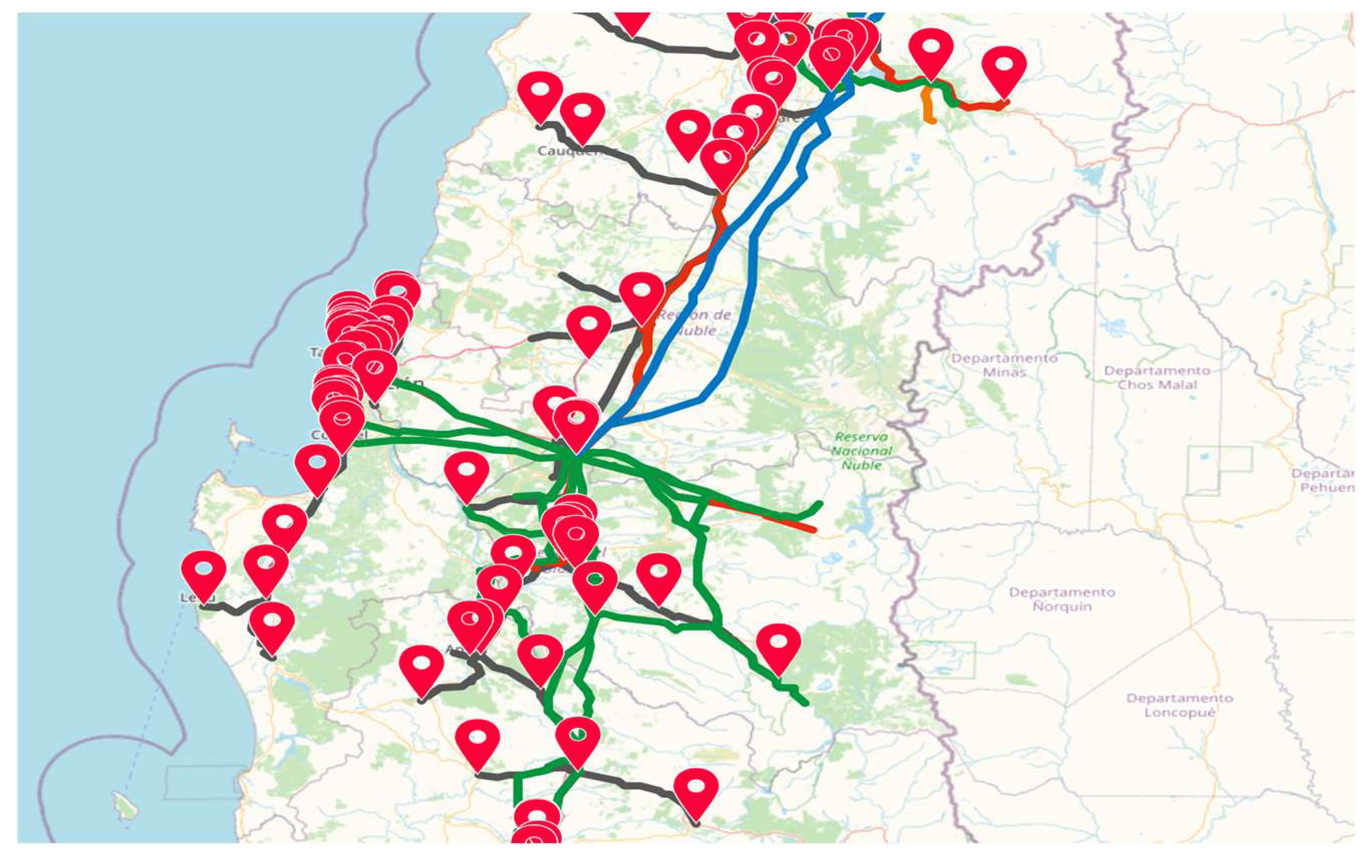
The Independent System Operator in Chile (known as Coordinador Eléctrico Nacional in Chile, hereinafter, the Coordinator) is the institution in charge of coordinating the operation of the National Electric System in a secure, economic and open-access way. Also, this institution has additional responsibilities inside the electrical sector. It is the system and market operator, participates in the power transmission planning, determines the available transmission capacity, monitors the capacity of the power system to meet the demand in the coming months, among other activities. Regarding transmission planning, every year, the Coordinator proposes new public work projects and the extension works that should be built in the future to the National Energy Commission (known as CNE in Chile). Then, the CNE takes this input and other inputs to determine the transmission expansion plan that will be developed in the coming years. In order to guarantee open access to new power plants, every year, the Coordinator determines the available transmission capacity of dedicated facilities. In all these tasks, the Coordinator uses different kinds of models to simulate the future operation of the power system, and it uses mathematical models to forecast the electric demand at the buses level. The electric demand projection is an input for these operation and planning models. In comparison to other energy and electric demand models where the projections are carried out at a national or regional level, here, more details are required to represent the electric demand and simulate the power flows of the network. Chile is divided into 16 regions and 346 districts. The power system model is represented by 636 buses distributed throughout these regions and districts. However, these buses do not represent the network after the primary substations in the distribution power systems. Figure 1 shows the geographical location of some of these buses in Chile.

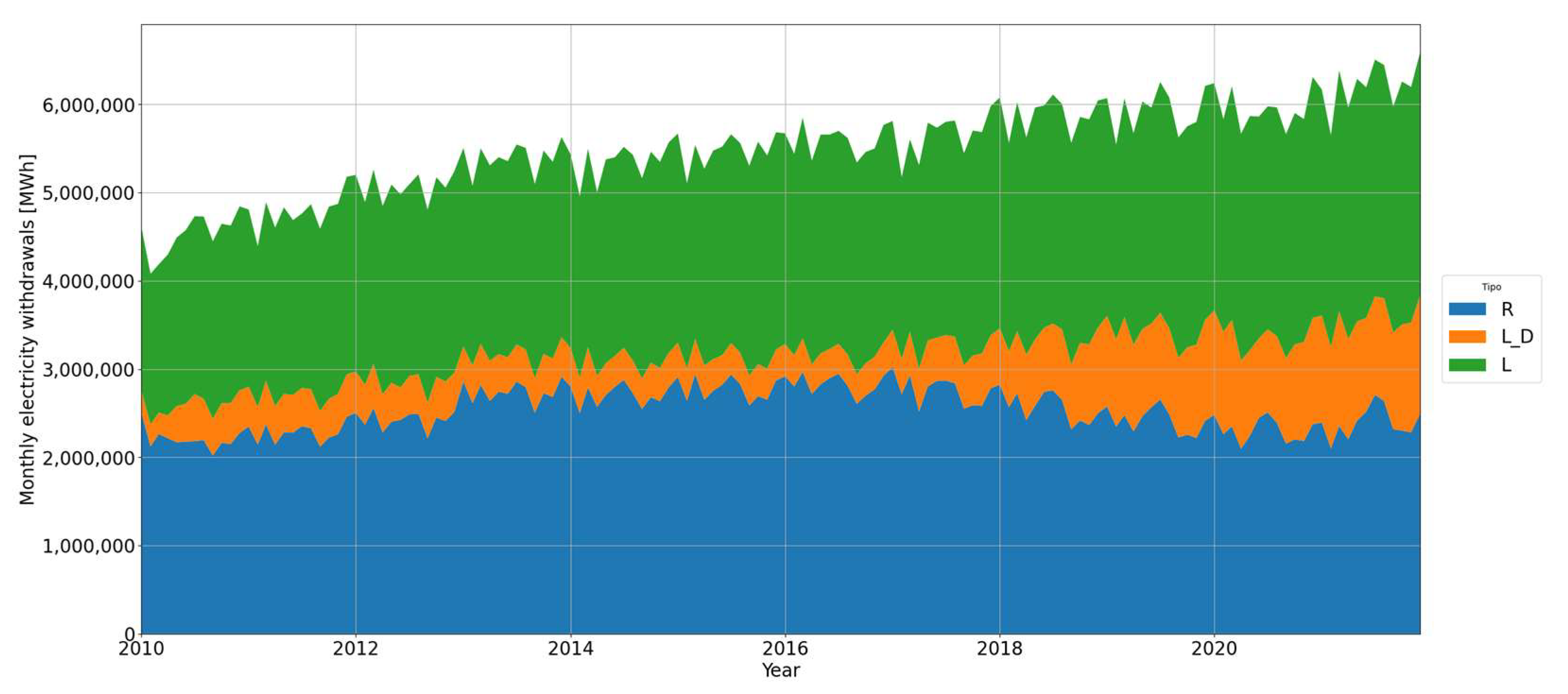
The electric demand of Chilean Electrical Power System (or SEN, as it is known in Chile) increased by an average of 4% annually between 2010 and 2021. The regulation authority in Chile classified the clients in two types: regulated and non-regulated clients. Electric demand for regulated clients is provided by retail companies. The non-regulated clients have more than 5000 kW of electric demand and can negotiate their power supply directly with generation companies. Some small non-regulated clients are connected to the distribution system. In addition, the current regulation allows regulated clients whose electric demand is between 500 kW and 5000 kW to become non-regulated clients. In fact, in recent years, an important share of regulated clients has become non-regulated clients in order to access energy at the best price. Figure 2 shows the historical monthly demand in Chile.

This paper aims to develop a methodology to forecast electrical demand for the Chilean Electrical Power System. The main contribution of this work is to develop an electricity demand projection model that considers bus spatial disaggregation, a topic that has not been extensively addressed in previous studies. Similarly, the proposed methodology combines the use of econometric models and end-use models to quantify the impact of decarbonization measures on the variation in electricity demand. This level of detail is required for the transmission planning activities carried out by the Coordinator. The methodology was implemented in the software DEMPRO-GIS 1.0 (Demand Projection—Geographic Information System) which was developed for the Coordinator in Chile and applied to project the electric demand for the period of 2022–2042 for 14 regions, 207 districts and 474 buses.

2. Energy Demand Models

From the literature review in [1], the techniques for projecting electricity demand can be classified into two large families, namely parametric models based on statistical techniques that analyze historical data on electricity demand and its relationship with the variables that affect it, and models based on artificial intelligence techniques such as neural networks, SVM, genetic algorithms, among others. Parametric models are based on finding statistical relationships between electricity demand and other variables that would affect demand levels. These methods have been used for a long time and have proven to be adequate to make demand forecasts. The problem with these models is that they are not able to represent complex and non-linear relationships between the forecasting variables and demand. The main techniques of these types of models are described below.

Trend analysis: These models seek to project the trend of the demand time series into the future, which can range from the most basic, such as projecting a trend line, to generating polynomials and more complex functions to project the trend. This approach is only based on projecting the demand curve without using additional variables. Its great advantage is that it is simple and quick to generate, while its disadvantage is that it only observes the trend of the demand curve without explaining the reasons for its behavior and the exogenous variables that could produce a change in this trend such as changes in prices or government policies.

End-use models: These models follow a bottom-up approach in which electricity demand is constructed through each of the end-use projections for this type of energy. These models, for example, analyze projections of electricity consumption in lighting, house heating, electrical motors, and so forth. The advantage of these models is that they tend to be quite accurate if performed well. However, they are very sensitive to the quality and quantity of the information used as input to these models. Generally, the quality of historical information disaggregated by end use is difficult to find or comes from approximations with a high margin of error. Additionally, historical and future changes in end-use shares depend on many factors such as changes in energy and device prices that are very difficult to predict.

Econometric models: These models combine economic theory and statistical techniques to predict electricity demand. These techniques analyze the relationships between electricity consumption and economic factors that explain this consumption. These models seek to generate a function that depends on economic, climatic, demographic, and other variables to explain changes in electricity demand. The advantage is that they produce detailed information on the future trend of electricity consumption, explaining the variables on which these changes depend. The disadvantage is that these models assume that these relationships with the explanatory variables remain constant over time, that is, they assume constant elasticity, which can be difficult to justify.

Artificial Intelligence Models: In addition to the traditional models mentioned above, new research in the development of demand forecasting models is reviewed in [2]. The article mentions that new types of probabilistic models and hybrid models between intelligent models and optimization algorithms are currently being developed. In the field of probabilistic models, we can mention Probabilistic Deep Learning (PDL), in which model parameters are described as a probability function; some of these types are the Bayesian Neural Network (BNN) and the Bayesian LSTM. Hybrid models seek to take advantage of the advantages of each individual model and create models that are more accurate and efficient. The most common models to be hybridized are artificial neural networks (ANNs) and support vector machines (SVMs). For neural networks, Neuro-Fuzzy (NF), ANN and Wavelet Transform (ANN-WT), ANN and Fruit Fly Optimization (ANN-FOA), ANN and Firefly Algorithm (ANN-FA), ANN and Particle Swarm Optimization (ANN-PSO), ANN and Artificial Immune System (ANN-AIS), ANN and Optimization Algorithms and ANN and Genetic Algorithms (GA). For SVMs, SVM and Particle Swarm Optimization (SVM-PSO), Least Square Support Vector Machine (LSSVM), SVM and Genetic Algorithms (SVM-GA), SVM and Fruit Fly Optimization (SVM-FOA) are mentioned. In our paper, a hybrid approach combining trend analysis and end-use models is proposed. This method leverages the strengths of both techniques to predict electricity demand trends, primarily driven by economic and population growth. Additionally, it incorporates emerging trends not typically addressed by these methods, such as the adoption of electric vehicles and the integration of electric generation within distribution networks, among others.

A comprehensive examination of techniques and technologies for forecasting energy demand is conducted in [3]. The methodologies discussed in this study encompass statistical, machine learning, and various ensemble methods. Through their analysis, the authors classify energy load forecasting based on the forecast horizon, ranging from very short (approximately one hour) to long-term (over one year). Statistical and linear models demonstrate greater efficacy for long-term horizons, whereas deep learning models excel in short-term forecasts. In terms of input parameters, weather and economic variables are the most utilized, featured in 50% of the literature, followed by historical energy consumption at 38.33%. The paper also delves into techniques for data collection and preprocessing.

The techniques described above have been used, both in academic papers and real-life applications. For example, [4] used a hybrid model (top-down and end-used models) to project the energy demand of the commercial sector in South Korea. They found that an intensity model is the most suitable for forecasting electricity demand for the commercial sector since econometric variables did not show statistical significance when trying out econometric models. In [5], a recurrent neural network LSTM is used to predict electrical demand in the region of New England. They did a long-term forecast (five years) with an hourly resolution. They used Random Forest models to identify relevant characteristics to predict electrical demand and found out that the calendar time was the most important variable (year, month, day), while climate variables were not as important. In [6], an end-use model is applied to forecast the electrical demand of the residential sector in Ethiopia, splitting the sector in urban–rural and electrified or not electrified. The demand of other economic sectors in Ethiopia were forecast using a top-down approach. In [7], a dynamic system is developed to forecast long-term electrical demand in order to comply with a carbon neutral scenario.

In [8], a methodology to identify relevant characteristics to predict electrical demand is proposed. They used climate and socioeconomic variables and found that the occurrence of the La Niña and El Niño phenomenon is a relevant characteristic to forecast electrical demand in Colombia. In [9], different time series are analyzed in order to forecast electrical demand in Brazil. The authors in this work developed regressive models with a stationarity, smooth exponential model and ARIMA models; they concluded that the ARIMA model was best-suited to predict electricity demand in their country, although it is recommended that a good amount of historical data be used to improve the performance of these kinds of models. The approach used in [10] was projecting electrical demand in Italy at a local scale (1 km2) based on population, land use, social and economic variables, and climate scenarios. They forecast the evolution of land use every 1 km2 in Italy depending on the projections of socioeconomic variables, then they project the electric intensity of the residential depending on GDP per capita and cooling degree days; both models are combined to forecast electrical consumption until 2050. The work presented in [11] assesses the projected energy efficiency improvements and potential energy savings within China’s 2060 carbon neutrality plan. The analysis leverages historical time series data on China’s primary energy demand, spanning from 1965 to the projected year 2060. Econometric techniques are then employed to establish the relationship between energy demand and influencing factors, such as economic growth and industrial structure. Finally, the study simulates various scenarios for primary energy demand in 2060, incorporating the plan’s energy efficiency targets. The results align with the findings of [11], suggesting that China’s carbon neutrality plan anticipates a moderate increase in primary energy demand by 2060 (approximately 14% higher than 2020). However, this increase is accompanied by significant projected improvements in energy efficiency, leading to substantial energy savings compared to a scenario without such measures. The study emphasizes the need for the robust implementation of energy efficiency policies to ensure the plan’s success and ultimately achieve China’s carbon neutrality goals.

In [12], an efficient model is presented that incorporates uncertainty forecasting and peer-to-peer trading, facilitating the dynamic matching of supply and demand while reducing electricity costs. This paper follows a trend analysis model, with a loop functionality between generation (supply), storage and consumption (demand). Ref. [13] compares three forecasting models: LGSSM (Linear Gaussian State-Space Model), FFNET (Feedforward Neural Network) and RF (Random Forest), with a baseline MLR (Multiple Linear Regression) models. It evaluates these different predictive models for electricity demand in urban areas, finding superior performance with linear Gaussian models in short-term (one step of 30 min ahead) forecasts and nonlinear autoregressive neural networks in long-term forecasts (48 steps ahead). Ref. [14] combines system dynamics (one kind of trend analysis) and power generation mix planning to forecast demand during the transition to low-carbon energy. In China, the results indicate a peak in CO₂ emissions in 2030 and emphasize the importance of maintaining a proportion of thermal power generators as backup.

The studies also explore various models incorporating temperature and other factors into forecasting, such as [15,16]. Ref. [15] compares how different treatments of weather affect load forecasting performance in short- and mid-term load forecasting models: time series methods (like linear regressions, Auto-Regressive Moving Average (ARMA) and ARMA with explanatory variables (ARMAX)) and feed-forward neural networks (FFNs). Ref. [16] evaluates for different time horizons (2, 5, and 10 years) and different time frequencies (days, months, and years) using ANN, ARIMA with Wavelet Transform or Fourier Transform. Further research includes models for optimizing microgrids and econometric models for predicting annual and quarterly consumption [17,18,19]. Ref. [17] ARMA models for scenario generation to capture uncertainties in consumption load, renewable energy output, and market prices, and uses the Kantorovich distance matrix method to reduce the number of scenarios, thereby managing computational complexity. Ref. [18] evaluates three classical econometric regression models: random parameter linear regression model (RPLRM), a correlated random parameter linear model (C-RPLRM), and a random parameter linear model with heterogeneity in means and variances (RP-HMV). Also, for comparison purposes, it estimates a multiple regression linear model and a data-driven time-series-based model, namely the grey model (GM). Ref. [19] develops a novel nonhomogeneous discrete grey model that considers seasonality by introducing a seasonal index into a fractional accumulation generation operator, which is abbreviated as SFNDHM. In [20], a hybrid model combines the grey model and Least Squares Support Vector Machine (LS-SVM) to improve forecasting accuracy and usability, providing insights into the spatial–temporal distribution of electrical consumption in Beijing. In ref. [21], the hybrid approach integrates data mining techniques and time series analysis, including Support Vector Regression (SVR), ARIMA, and neural networks. This study aims to minimize errors in the long-term forecasting of electric peak load and energy demand.

As explained above, in comparison to previous works, the proposed methodology in this paper is based on a combination of econometric and end-use models, which we describe in Section 3. In addition,

Table 1. Comparison of different approaches regarding spatial disaggregation, temporal resolution, forecasting horizon, and the representation of low-carbon technologies modeled with end-use models.

Reference	Spatial Disaggregation	Temporal Resolution	Forecasting or Predictions Horizon	Low-Carbon Technologies Modeled with End-Use Models
[4]	national	annual	2019–2030	No
[5]	state	hourly	2011–2015	No
[6]	national	annual	2018–2050	Energy efficiency scenario included.
[7]	national	annual	2020–2060	No
[8]	one region	monthly	2015–2017	No
[9]	regional	monthly	5 years	No
[10]	grid cells of 1 km × 1 km	annual	2018–2050	No
[11]	national	annual	2020–2060	No
[12]	microgrid	hourly	A week	Distributed generation
[13]	city, district	minutes	A day	No
[14]	national	annual	2020–2035	Electromobility
[15]	regional	daily	A week	No
[16]	national	daily, monthly, annual	2, 5, or 10 years (2009, 2014, 2017–2019).	No
[17]	microgrid	hourly	A day	No
[18]	national	annual	2020–2031	No
[19]	city	quarterly	2010 Q4–2019 Q3	No
[20]	district	annual	2020–2024	No
[21]	national	annual	2017–2026	No
This paper	regional, district and buses	monthly	20 years (2022–2042)	Electromobility, distributed generation, electric heating, electric cooking, air conditioning.

shows a comparison of different approaches regarding spatial disaggregation, temporal resolution, forecasting horizon, and the representation of low-carbon technologies modeled with end-use models.

In Chile, there are some previous works related to electric demand projection. The Coordinator periodically forecasts electrical demand in the country to make use of the projection for several long-term studies such as the power transmission planning proposal of the Chilean Electrical Grid, among others. The last electrical demand projection model was developed in 2018 [22]. That model is based on an econometric model that seeks to capture the relationship between electricity demand and its main explanatory variables, and to forecast electricity consumption consistent with the expected patterns for these variables. The electrical demand is disaggregated into demand from non-regulated and regulated customers. Non-regulated customers are disaggregated into the copper mining industry and all other industries. Unlike the work that is shown in this paper (see next methodology section), the projection carried out in 2018 did not disaggregate non-regulated clients into more economic sectors, other than the copper industry, and did not consider new technologies and changes in customers’ behaviors such as electromobility, electrification in the residential sector, distributed generation, etc. with the detail as carried out in this work. Also, several improvements were introduced to the software that computes electrical demand projections and the software that shows the projections at the bus level with accurate georeferentiation.

Other works related to electricity projections in Chile are the Long-Term Energy Planning report carried out by the Energy Ministry [23]. This report utilizes an end-use model to project not only electricity but also other types of energy consumption such as transportation fuel, coal and natural gas in the industry, and firewood for heating in the residential sector, among others. It serves as a key input for several public policy studies in the country. This report does not forecast electric demand considering a bus spatial disaggregation, as is performed in this paper. Additionally, the National Energy Commission produces its own report, as described in the introduction, which is based on the projections carried out by the Coordinator [24]. Furthermore, COCHILCO (Chilean copper corporation) conducts electricity projection specifically for the copper mining industry [25], and some utility companies project electricity demand in their respective concession areas [26].

In the following section, we describe, in more detail, the developed methodology and use of econometric models and end-use models.

3. Methodology

3.1. Overview Description

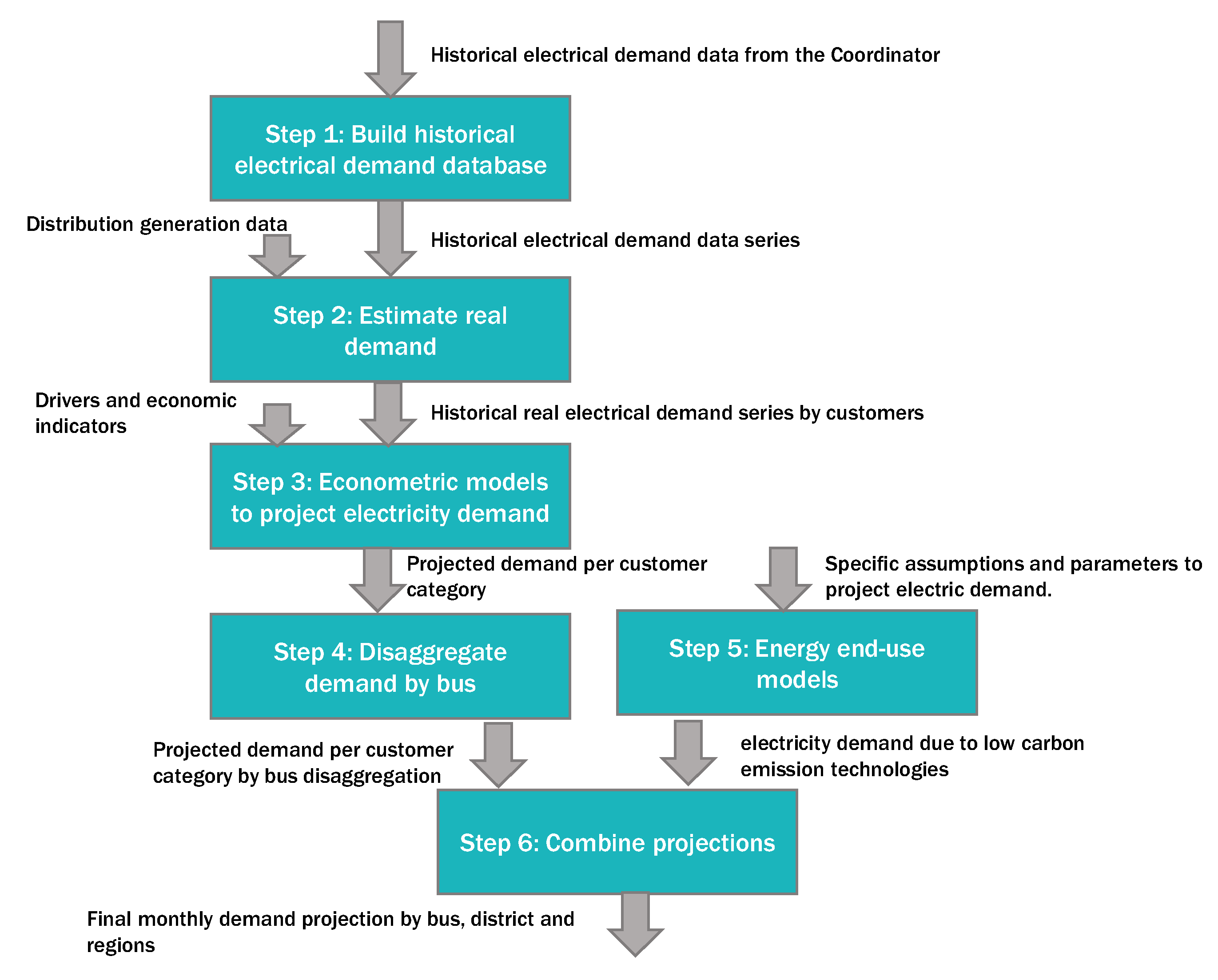
The methodology developed was based on different econometric models and end-use models to represent the massification of low-carbon emission technologies. The steps of the proposed methodology are shown in Figure 3, and their inputs and main process are described as follows.

Step 1. Build historical electrical demand database: The initial step aims to build a database containing historical electrical demand data at the bus level.

Inputs: Historical electrical demand data from the Coordinator (2010–2021)

Process: Using the historical data provided by the Coordinator, we compiled a database with the demand for the period from 2010 to 2021.

Step 2. Estimate real demand: Since distributed generation decreases the electric demand reported by clients to the Coordinator, we estimate the real demand adding to the demand the effect of the distributed generation.

Inputs: Historical electrical demand data, distribution generation data.

Process: Estimate distribution generation using installed capacity and renewable energy resources and calculate real demand. Real demand is calculated as the historical demand plus distribution generation. More details of this step are described in Section 3.2.

Step 3. Econometric models to project electricity demand: Electricity demand for every customer category is projected using econometric models. Customers were categorized into three groups: (1) regulated and non-regulated clients connected in distribution areas, (2) copper-mining customers, and (3) other industrial customers from cement, iron ore mining industries, etc.

Inputs: Customer category economic indicators (IMACEC, population, housing, electricity price), historical real electrical demand series.

Process: For each customer category, we develop an econometric model to project demand based on economic indicators. More details of this step are described in Section 3.2, and in Section 3.5, there are more details of drivers and economic indicators.

Step 4. Disaggregate demand by bus: Electricity demand is projected considering bus spatial disaggregation.

Inputs: Projected demand per customer category.

Process: Allocate projected demand to specific buses based on the results of econometric models, or other assumptions.

Step 5. Energy end-use models: In this step, we quantify the impact of the massification of low-carbon emission technologies such as electromobility, electric heating, electric heating water, and distributed generation.

Inputs: Every end-use model uses specific assumptions and parameters to project electric demand.

Process: Forecast the effect of low carbon emissions on electricity demand. More details of this step are described in Section 3.5.

Step 6. Combine projections: Finally, we combine the results of econometric and end-use models to forecast the electric demand.

Inputs: Projected demand by bus from econometric models and end-use models.

Process: Combine all projections to obtain a final monthly demand projection by bus. The results of applying this methodology are shown in Section 4.

3.2. Distributed Generation and Estimation of Historical Real Demand

In Chile, the distributed generation is classified in two types: SMDG (Small and Medium Distributed Generation, or PMGD in Spanish) and small projects under the net billing regulation. A SMDG project is a power plant which can inject its energy into the distribution system up to 9 MW. A net billing project has, as its maximum, 300 kW of capacity. There is a database with the SMDG injection into the distribution system at the bus level. Regarding the net billing projects, there is a database with the installed capacity but there is no information about their generation. So, we estimated the generation using the installed capacity and the renewable energy resources available in different districts. Then, with the injection of the SMDG and net billing projects, and the demand, it was possible to estimate real demand at the bus level.

The electric demand reported by non-regulated clients and distribution companies implicitly incorporates the effect of distributed generation, both from SMDG and projects under the net billing regulation. To obtain the actual demand at each substation, it is necessary to quantify the energy contributed by distributed generation. Ideally, econometric models should be estimated using the actual demand, for which the following procedure is proposed to estimate this demand. Once the projection of the actual demand is made, the estimation of distributed generation will be added exogenously, and the net demand projection will be calculated. The methodology to obtain the historical generation of SMDG and to estimate the historical generation of net billing is described below, and presents the necessary values for the calibration of econometric models. Additionally, the criteria used for the projection are mentioned.

3.2.1. SMDG Generation

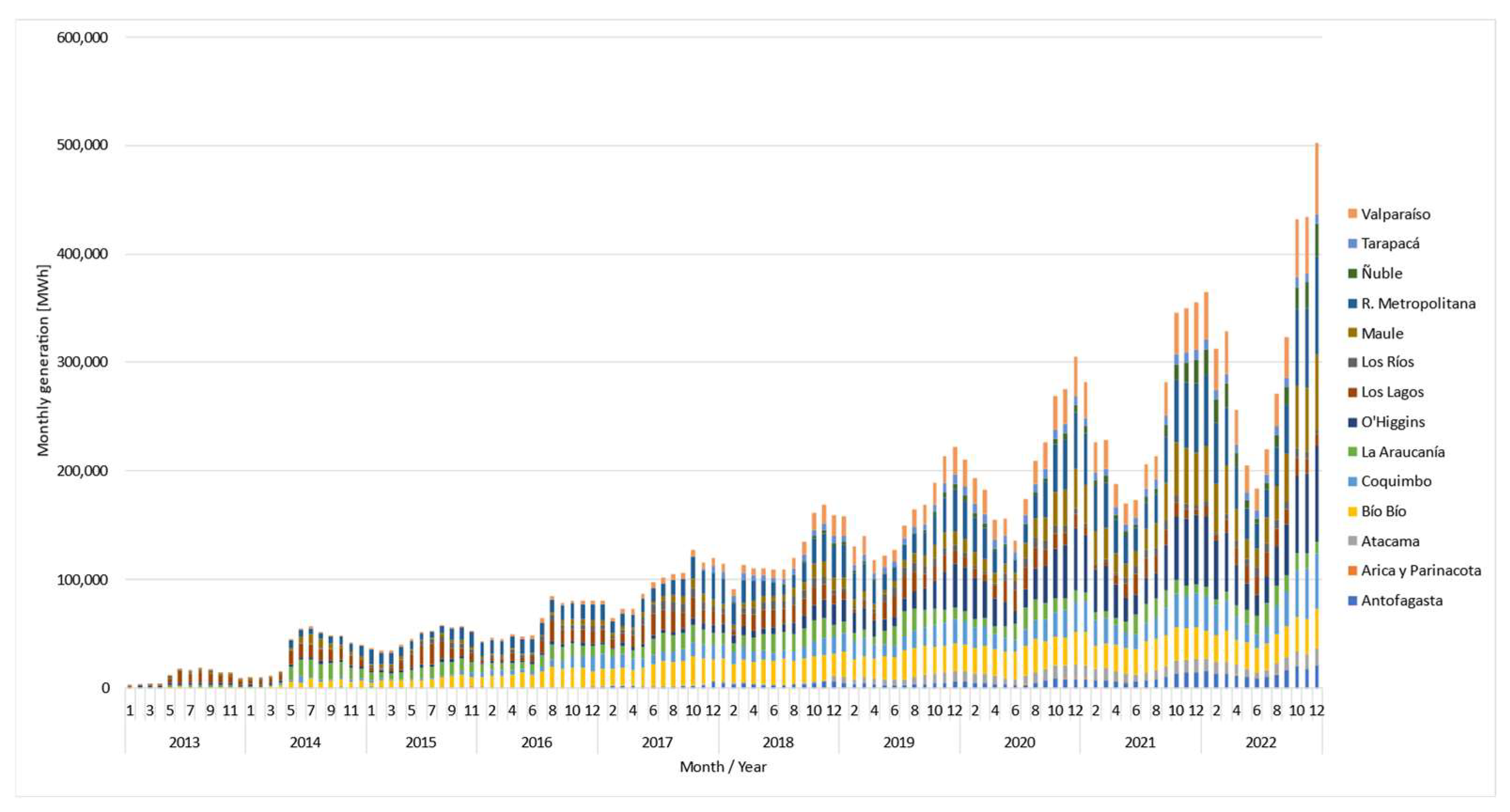
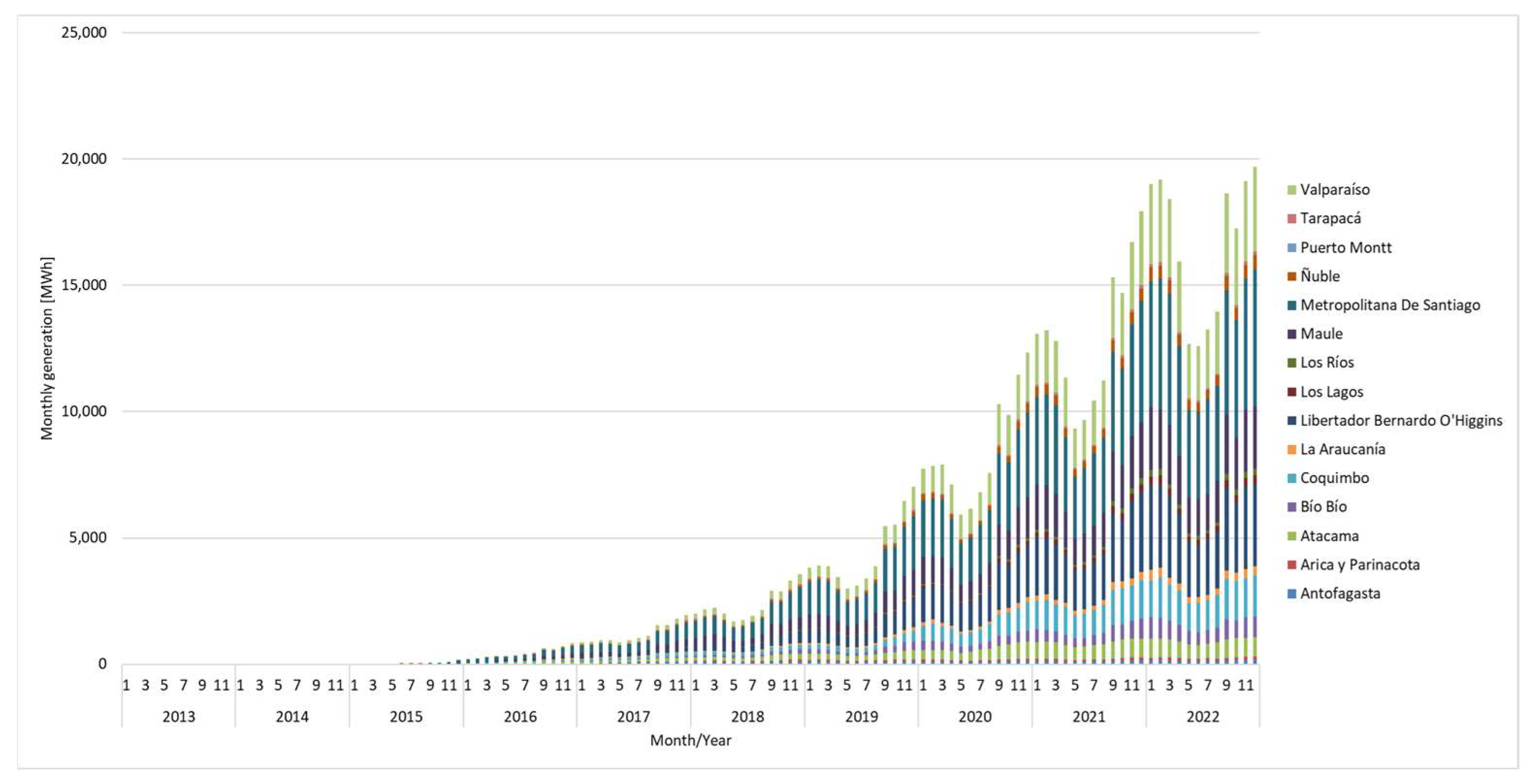
The historical generation of SMDG projects is obtained from the Calculation Backgrounds for Economic Transfers, published by the Coordinator. From the energy withdrawal information, power plants with energy injections (or negative consumptions) are identified, along with their respective year, month, and connection point. Then, to integrate historical generation into the demand projection model, the power plants were assigned to the existing substations or nodes in the electric demand data. Figure 4 and Figure 5 show the historical generation of SMGD power plants by technology and by region, respectively.

The modeling of the SMDG power plant projection is represented by power plants in operation, under construction, or with approval as of 2021. New plants are included at the end of the period as an assumption, but with a lower growth rate than the plants about to be installed.

3.2.2. Net Billing Projects Generation

For net billing projects, since there is no monthly record of the energy injection from each residential and commercial project, a historical generation estimate was made based on the installed capacity of each project, an estimated plant factor, and the month of operation start. For solar photovoltaic technology, there is a monthly profile of the plant factor for each district, while for other technologies, there is an assumed constant plant factor of 0.3 associated with mini-hydro and thermal technologies.

Once the generated energy from each project is obtained, it is grouped by district. Then, the energy is distributed among the feeders located in the district in proportion to the capacity of each feeder. If a district does not have feeders, the feeders from the nearest district are assigned. Figure 6 shows the estimated historical generation of net billing projects, by region.

The modeling of the net billing projected capacity in the residential and commercial sectors is carried out following a Bass model, that is, establishing a probabilistic relationship between the adoption of the technology by a part of the population defined as the innovator, and the adoption by the other part of the population, defined as the imitator.

3.2.3. Estimation of Historical Real Demand

Figure 7 shows the effect on demand of distributed generation contribution. The black line represents the reported withdrawal data by customers. The yellow line represents the electric demand plus generation from net billing projects. Finally, the red line represents the estimated real demand considering the contribution of generation from net billing projects and the SMDG described above.

3.3. Econometric Models to Project Electricity Demand

3.3.1. Regulated and Non-Regulated Clients in Distribution

The following econometric model was developed to project the electric demand for regulated and non-regulated clients in the distribution power system. We explore the relationship between demand and the price of energy, an index to represent the monthly index of economic activity (IMACEC for its acronym in Spanish), the number of dwellings, and the population. A dummy variable COVID was included to capture the effect of the pandemic:

$$Q_{i,t}={\beta }_1\times P_t+{\beta }_{2,r\left(i\right)}\times {IMA}_t+{\beta }_3\times {VIV}_{c\left(i\right),t}+{\beta }_4\times {POB}_{c\left(i\right),t}+\sum _j{\beta }_j{B}_j+COVID \forall i,t$$

where

• $Q_{i,t}$: Electric demand in bus i and in month t;
• $P_t$: Price of the electricity in month t;
• ${IMA}_t$: IMACEC in month t;
• ${VIV}_{c\left(i\right),t}$: Number of dwellings in district c (district where the bus i is) in the month t;
• ${POB}_{c\left(i\right),t}$: Population in district c (district where the bus i is) and in month t;
• $B_j$: Binary variable equals 1 if bus j equals bus i, 0 otherwise;
• ${\beta }_j$: Fix coefficient for bus j.
• ${\beta }_1,{\beta }_{2,r\left(i\right)},{\beta }_3,{\beta }_4$: Elasticity regarding the explored variables; in the case of the elasticity on IMACEC (${\beta }_{2,r\left(i\right)}$), this may have a different value for each region of Chile (r) where the bus (i) is located.

Different models were produced as a combination of these variables: $P_t,{ IMA}_t$, ${VIV}_{c\left(i\right)t}$, and ${POB}_{c\left(i\right)t}$. The detailed results of the econometric models, including R² values, the number of observations, and p-values for each coefficient, are shown in Appendix A. For the regulated and non-regulated clients in distribution, 15 models were estimated (see

Table A1. Regulated and non-regulated clients in distribution. Part 1.

	(1)	(2)	(3)	(4)	(5)	(6)
	Log_E	Log_E	Log_E	Log_E	Log_E	Log_E
Log_P	−0.145 *	−0.144 *	−0.136 *	−0.153 *	−0.173 **	−0.159 *
	(0.019)	(0.023)	(0.030)	(0.014)	(0.006)	(0.012)
Log_IMA	0.838 ***	0.841 ***	0.851 ***	0.827 ***	0.794 ***	0.813 ***
	(0.000)	(0.000)	(0.000)	(0.000)	(0.000)	(0.000)
covid	0.0386 ***	0.0392 ***	0.0403 ***	0.0373 ***	0.0331 **	0.0352 ***
	(0.000)	(0.000)	(0.000)	(0.000)	(0.002)	(0.001)
Log_P_D_2016	1.094 ***	1.098 ***	1.105 ***	1.086 ***	1.045 ***	1.059 ***
	(0.000)	(0.000)	(0.000)	(0.000)	(0.000)	(0.000)
D_desde_2016	−4.409 ***	−4.426 ***	−4.450 ***	−4.379 ***	−4.218 ***	−4.269 ***
	(0.000)	(0.000)	(0.000)	(0.000)	(0.000)	(0.000)
Log_POB		0.207 *		0.108	0.361 ***
		(0.011)		(0.178)	(0.000)
Log_VIV		−0.204 **	−0.109		6.302 ***	6.124 ***
		(0.002)	(0.102)		(0.000)	(0.000)
Log_VIV2					−0.311 ***	−0.295 ***
					(0.000)	(0.000)
_cons	5.623 ***	5.373 ***	6.567 ***	4.571 ***	−29.34 ***	−25.49 ***
	(0.000)	(0.000)	(0.000)	(0.000)	(0.000)	(0.000)
N	27968	27968	27968	27968	27968	27968
r2_a	0.923	0.923	0.923	0.923	0.923	0.923

Controles: C; * p < 0.05, ** p < 0.01, *** p < 0.001.

). The results shown in Section 4 were obtained using model n°14. The models shown in Appendix A have 27,968 observations for busbars in 402 electric substations in 202 districts in Chile.

3.3.2. Copper-Mining Clients

The following econometric model was developed to project the electric demand for copper-mining industries. We explore the relationship between electric demand for mining companies and mining production, an index to represent the monthly mining economic activity (mining IMACEC) and price of the electricity:

$$Q_{m,t}={\beta }_1\times P_t+{\beta }_2\times {IMAM}_t+{\beta }_3\times {PR}_{m,t}+\sum _n{\beta }_n{E}_n \forall m,t$$

where

• $Q_{m,t}$: Electric demand for the mining company m and in month t;
• $P_t$: Price of the electricity in month t;
• ${IMAM}_t$: Mining IMACEC in month t;
• ${PR}_{m,t}$: Copper production (or processed material) for the mining company m and in month t;
• $E_n$: Binary variable equals 1 if company n equals company m, 0 otherwise;
• ${\beta }_n$: Fix coefficient for company n;
• ${\beta }_1,{\beta }_2,{\beta }_3$: Elasticity regarding the explored variables.

Different models were analyzed considering more or less explanatory variables than those mentioned above. For example, models that only include copper production and the price of electricity were studied. Models that use processed material instead of copper production as an explanatory variable are also analyzed. Energy consumption depends on the processed material, and it depends on the copper grade. In this way, the model could represent the impact of the decrease in the copper grade that is expected for the upcoming years. The final variables selected for each model depend on the quality of the econometric model estimators. For this sector, four models were developed, and

Table A3. Copper mining.

	(1)	(2)	(3)	(4)
	Log_E	Log_E	Log_E	Log_E
Log_procesado_CU	0.653 ***		0.652 ***
	(0.000)		(0.000)
Log_CU		0.589 ***		0.604 ***
		(0.000)		(0.000)
covid			0.0520 ***	0.105 ***
			(0.000)	(0.000)
_cons	5.826 ***	9.454 ***	5.825 ***	9.392 ***
	(0.000)	(0.000)	(0.000)	(0.000)
N	2485	2485	2485	2485
r2_a	0.923	0.912	0.923	0.914

Controles: Empresa+Mes; *** p < 0.001; Log_procesado_CU: Logarithm of processed copper ore (${PR}_{mt}$); Log_CU: Logarithm of copper production (${PR}_{mt})$; COVID: Dummy variable indicating the pandemic period.

in Appendix A contains the details of the estimated econometric models. The models shown in Appendix A have 2485 observations for 24 copper-mining sites in Chile.

The results shown in Section 4 were obtained using model n°1. The electricity demand projection was then distributed by bus according to the observed historical participation of each mining company.

3.3.3. Other Industries and Commercial Clients

Different econometric models were developed to project the electric demand for other industries (steel industry, pulp and paper industry, cement industry, iron mining, other industries, other mining, and petrochemical industry) and the commercial sector. These sectors are part of the non-regulated clients which are not connected to the grid in the distribution system (in Chile also known as “cliente libre”). We explore the relationship between electric demand and the industrial production of these sectors, an index to represent the monthly industry economic activity (IMACEC), and the price of the electricity. For every sector, we developed a model as follows:

$$Q_{s,t}={\beta }_{1,s}\times P_t+{\beta }_{2,s}\times {IMA}_t+{\beta }_{3,s}\times {PR}_{s,t}+{\beta }_{4,s} \forall s,t$$

• $Q_{s,t}$: Electric demand for the sector s and in month t;
• $P_t$: Price of the electricity in month t;
• ${IMA}_t$: IMACEC in month t;
• ${PR}_{s,t}$: Industrial production for the sector s and in month t;
• ${\beta }_{1,s},{\beta }_{2,s},{\beta }_{3,s},{\beta }_{4,s}$: Elasticity regarding the explored variables.

For every sector, historical information of industrial production was obtained from different information sources. Afterwards, the electricity demand projection was distributed by bus according to the observed historical participation of each industrial sector. The developed models for each economic sector are shown in

Table A4. Steel industry.

	(1)	(2)
	Log_E	Log_E
Log_Siderurgia	0.667 ***	0.282 **
	(0.000)	(0.003)
D_2010	−1.339 ***
	(0.000)
Log_P	−0.962 ***	−1.691 **
	(0.000)	(0.006)
L.Log_E		0.529 ***
		(0.000)
L2.Log_E		0.137 *
		(0.027)
L3.Log_E		−0.137 **
		(0.002)
Log_IMA_IND		0.206
		(0.214)
L.Log_IMA_IND		−0.480 **
		(0.003)
L.Log_P		1.341 *
		(0.027)
_cons	9.630 ***	5.580 ***
	(0.000)	(0.000)
N	132	128
r2	0.741	0.812

p-values in parentheses * p < 0.05, ** p < 0.01, *** p < 0.001; Log_Siderurgia: Logarithm of steel production ($Q_{st})$; D_2010: Dummy variable for the year 2010; Log_P: Logarithm of the electricity price ($P_t$); L.Log_E: Logarithm of electricity demand lagged by one year; L2.Log_E: Logarithm of electricity demand lagged by two years; L3.Log_E: Logarithm of electricity demand lagged by three years; Log_IMA_IND: Logarithm of the industrial IMACEC (economic activity index for the industrial sector); L.Log_IMA_IND: Logarithm of the industrial IMACEC lagged by one year; L.Log_P: Logarithm of the electricity price lagged by one year.

,

Table A5. Pulp and paper industry.

	(1)	(2)
	Log_E	Log_E
Log_celulosa	−0.639 *	−0.217
	(0.014)	(0.221)
Log_IMA_IND	0.244	0.357 **
	(0.372)	(0.008)
Log_P	−0.198
	(0.087)
L.Log_E		0.776 ***
		(0.000)
L.Log_IMA_IND		−0.370 **
		(0.007)
_cons	17.12 ***	4.593 **
	(0.000)	(0.004)
N	132	128
r2	0.0789	0.687

p-values in parentheses; * p < 0.05, ** p < 0.01, *** p < 0.001; Log_celulosa: Logarithm of pulp production ($Q_{st})$; Log_P: Logarithm of the electricity price ($P_t$); Log_IMA_IND: Logarithm of the industrial IMACEC (economic activity index for the industrial sector).

,

Table A6. Cement industry.

	(1)	(2)
	Log_E	Log_E
Log_cemento	1.003 ***	0.658 ***
	(0.000)	(0.000)
Log_IMA	0.566 ***	0.332 **
	(0.000)	(0.001)
Log_P	−0.0979
	(0.368)
L.Log_E		0.384 ***
		(0.000)
_cons	−0.347	−0.721
	(0.839)	(0.586)
N	144	140
r2	0.321	0.412

p-values in parentheses; * p < 0.05, ** p < 0.01, *** p < 0.001; Log_cemento: Logarithm of cement production ($Q_{st})$; Log_P: Logarithm of the electricity price ($P_t$); Log_IMA: Logarithm of IMACEC (economic activity index) (${IMA}_t$); L.Log_E: Logarithm of electricity demand lagged by one year.

,

Table A7. Commercial sector.

	(1)	(2)	(3)
	Log_E	Log_E	Log_E
Log_P	0.411 ***
	(0.000)
Log_IMA	0.819 ***	1.126 ***	0.692 ***
	(0.000)	(0.000)	(0.000)
D_2019	−0.176 ***	−0.115 ***	−0.0613 ***
	(0.000)	(0.000)	(0.001)
L.Log_E			0.515 ***
			(0.000)
_cons	3.985 ***	4.271 ***	1.404 **
	(0.000)	(0.000)	(0.003)
N	120	120	119
r2	0.675	0.617	0.769

p-values in parentheses; ** p < 0.01, *** p < 0.001; Log_P: Logarithm of the electricity price ($P_t$); Log_IMA: Logarithm of IMACEC (economic activity index) (${IMA}_t$); D_2019: Dummy variable for the year 2019; L.Log_E: Logarithm of electricity demand lagged by one year.

,

Table A8. Iron mining.

	(1)	(2)
	Log_E	Log_E
Log_hierro	0.569 ***
	(0.001)
Log_IMA	0.228	0.382 **
	(0.273)	(0.004)
D_2016_2019	0.258 ***
	(0.000)
L.Log_E		0.725 ***
		(0.000)
_cons	4.567 ***	1.260 *
	(0.000)	(0.039)
N	144	140
r2	0.502	0.673

p-values in parentheses; * p < 0.05, ** p < 0.01, *** p < 0.001; Log_hierro: Logarithm of iron production ($Q_{st})$; Log_IMA: Logarithm of IMACEC (economic activity index) (${IMA}_t$); D_2016_2019: Dummy variable for the period 2016–2019; L.Log_E: Logarithm of electricity demand lagged by one year.

,

Table A9. Other industries.

	(1)	(2)
	Log_E	Log_E
Log_IMA	2.214 ***	0.660 **
	(0.000)	(0.002)
D_2010	−0.947 ***
	(0.000)
L.Log_E		0.640 ***
		(0.000)
L.Log_IMA		−0.571 *
		(0.019)
L2.Log_IMA		0.710 ***
		(0.001)
_cons	1.048	0.375
	(0.185)	(0.504)
N	144	140
r2	0.720	0.808

p-values in parentheses; * p < 0.05, ** p < 0.01, *** p < 0.001; Log_IMA: Logarithm of IMACEC (economic activity index) (${IMA}_t$); D_2016_2019: Dummy variable for the period 2016–2019; L.Log_E: Logarithm of electricity demand lagged by one year; L.Log_IMA: Logarithm of economic activity lagged by one year; L2.Log_IMA: Logarithm of economic activity lagged by two years.

,

Table A10. Other mining industries.

	(1)	(2)	(3)	(4)
	Log_E	Log_E	Log_E	Log_E
L.Log_E	0.730 ***		0.734 ***
	(0.000)		(0.000)
Log_IMA	0.325 *	0.557 **	0.257 *	0.397 **
	(0.012)	(0.001)	(0.013)	(0.005)
Log_P	−0.102	−0.243
	(0.337)	(0.118)
D_2016_2020	−0.156 **	−0.508 ***	−0.153 **	−0.506 ***
	(0.003)	(0.000)	(0.003)	(0.000)
_cons	1.754 *	8.836 ***	1.602 *	8.563 ***
	(0.028)	(0.000)	(0.036)	(0.000)
N	143	144	143	144
r2	0.836	0.614	0.835	0.609

p-values in parentheses; * p < 0.05, ** p < 0.01, *** p < 0.001; Log_IMA: Logarithm of IMACEC (economic activity index); L.Log_E: Logarithm of electricity demand lagged by one year; Log_P: Logarithm of the electricity price ($P_t$); D_2016_2020: Dummy variable for the period 2016–2020.

and

Table A11. Petrochemical industry.

	(1)
	Log_E
L.Log_E	0.235 ***
	(0.000)
Log_IMA	−0.695
	(0.066)
Log_P	−1.199 ***
	(0.000)
D201610	−1.512 ***
	(0.000)
D202006	−0.849 ***
	(0.001)
D201509	1.796 ***
	(0.000)
D201411	1.894 ***
	(0.000)
_cons	14.31 ***
	(0.000)
N	119
r2	0.735

p-values in parentheses; *** p < 0.001; Log_IMA: Logarithm of IMACEC (economic activity index); L.Log_E: Logarithm of electricity demand lagged by one year; Log_P: Logarithm of the electricity price ($P_t$); D201610: Dummy variable for October 2016; D202006: Dummy variable for June 2020; D201509: Dummy variable for September 2015; D201411: Dummy variable for November 2014.

in Appendix A. Model number 1 was chosen for each economic sector, but the steel industry and the commercial were chosen for model 2. Additional dummy variables were added in some econometric models. Lagged versions of these variables were also tested. The models shown in Appendix A have between 119 and 144 observations; depending on the industry, the amount of available historical data, and if lagged variables were used.

3.4. Energy End-Use Model

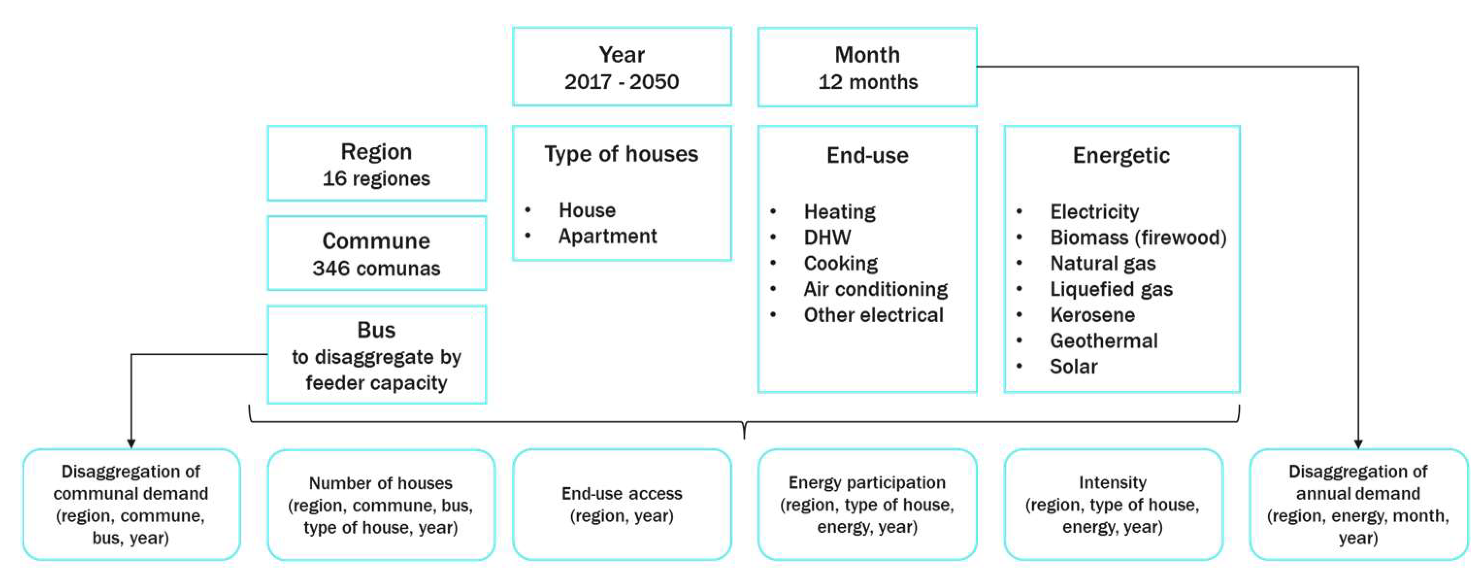
Currently, in Chile, there is an energy policy promoting the development of low-carbon emission technologies to achieve carbon neutrality by 2050 [27]. Due to the econometric models described above, it may not adequately capture the effect of these technologies; projections will need to consider the inclusion of new energy requirements that could affect demand projections. Examples include the electrification of residential consumption (e.g., the increased use of electric heating, air conditioning, etc.), public and private electromobility, energy efficiency, hydrogen production, etc. These electric demand projections will be performed using an end-use model, and then these projections will be added to the projections obtained with the econometric models. Figure 8 shows the general methodology.

The proposed methodology allows for the characterization of energy demand considering all energy sources and the most representative end-uses: heating, hot water, cooking, and electrical appliances. This approach enables the characterization of the increase in electrical demand resulting from the electrification of heating systems, the expected replacement of firewood in the central–southern zone of the country, the electrification of hot water systems, the electrification of cooking systems, and the increased electrical demand due to air conditioning use.

Based on the growth of the number of homes, the characterization of energy consumption in homes, and their energy end uses (heating, hot water, electrical appliances, etc.), it is possible to make annual energy demand projections for each district using the following expression:

$$E_{r,c,v,u,e,y}=N_{r,c,v,y}\times I_{r,v,u,e,y}\times A_{r,v,u,y}\times P_{r,v,u,e,y}$$

where

• $E_{r,c,v,u,e,y}$: Energy demand in region r, district c, type of housing v (house or apartment), end-use u, energy source e, and year y;
• $N_{r,c,v,y}$: Number of homes according to region r, district c, type of housing v, and year y;
• $I_{r,v,u,e,y}$: Energy intensity of each end-use u (expressed in kWh/home) according to region r, type of housing v, energy source e, and year y;
• $A_{r,v,u,y}$: Access to end-use u, for each region r, type of housing v, and year y;
• $P_{r,v,u,e,y}$: Participation of each energy source e in end-use u, according to region r, type of housing v, and year y.

The general methodology considers disaggregated information at a temporal level (year and month), spatial level (region, district, and bus), and energy level (end use and energy sources). This work uses two previous studies carried out by the researchers from the Energy Center: the residential sector database created for Long-Term Energy Planning (PELP, as it is known in Chile) during the 2018–2022 period [28], and the STEP 3.0 model [29] used for transportation sector projections. The first is mainly used for energy calculations and reference values, and the second is used for data structure and processing. For the energy intensities and participation of each energy source in different end uses, and the level of access of dwellings to energy services, information from the study on energy use in Chilean dwellings [30] and the trajectories developed by the Energy Center for the PELP 2018–2022 are used. Then, to update and calibrate the information with the latest official results, the intensity values are weighted until achieving the same energy consumption by energy source and region, as presented in the Regional Energy Balances, using average intensity values for the projection.

From the below equation, it is possible to obtain the monthly energy values t and per bus i, weighted by temporal and spatial distribution factors ($d_t$ and $d_i$, respectively).

$$E_{r,c,b,u,e,y,t}=E_{r,c,u,e,y}\times d_t\left[\%\right]\times d_i[\%]$$

An expected electrification of heating, cooking, and domestic hot water (DHW), and an increase in access to air conditioning in Chilean dwellings are modeled. This responds to decarbonization processes and access to more efficient technologies.

3.5. Driver Projections

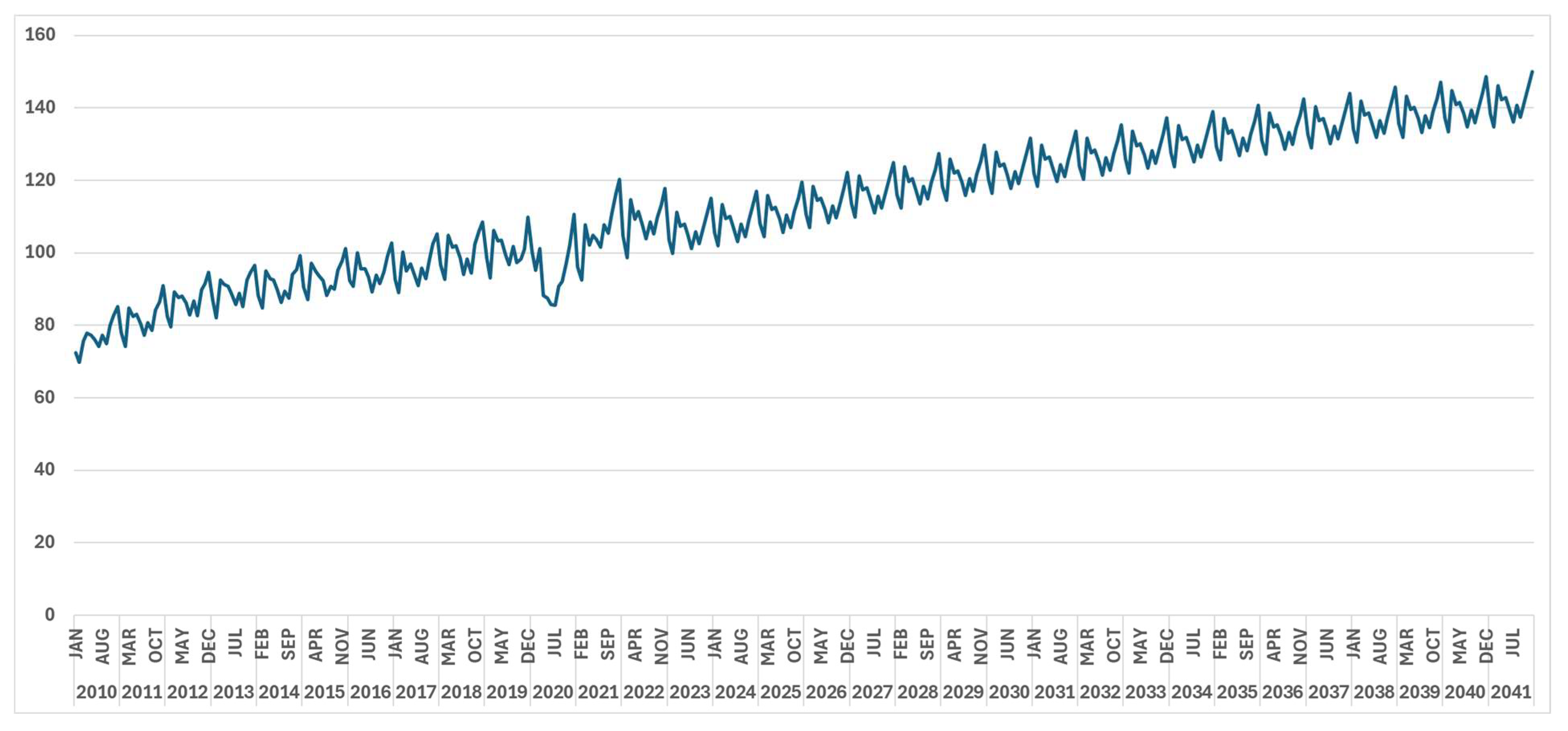
The developed models have, as input, several drivers. The economic growth, represented by the IMACEC index, population and housing, are used as input for the regulated sector and non-regulated sector in the distribution areas. The IMACEC projection is based on the information provided by the Ministry of Finance and OECD (2021). The following Figure 9 shows the IMACEC projection.

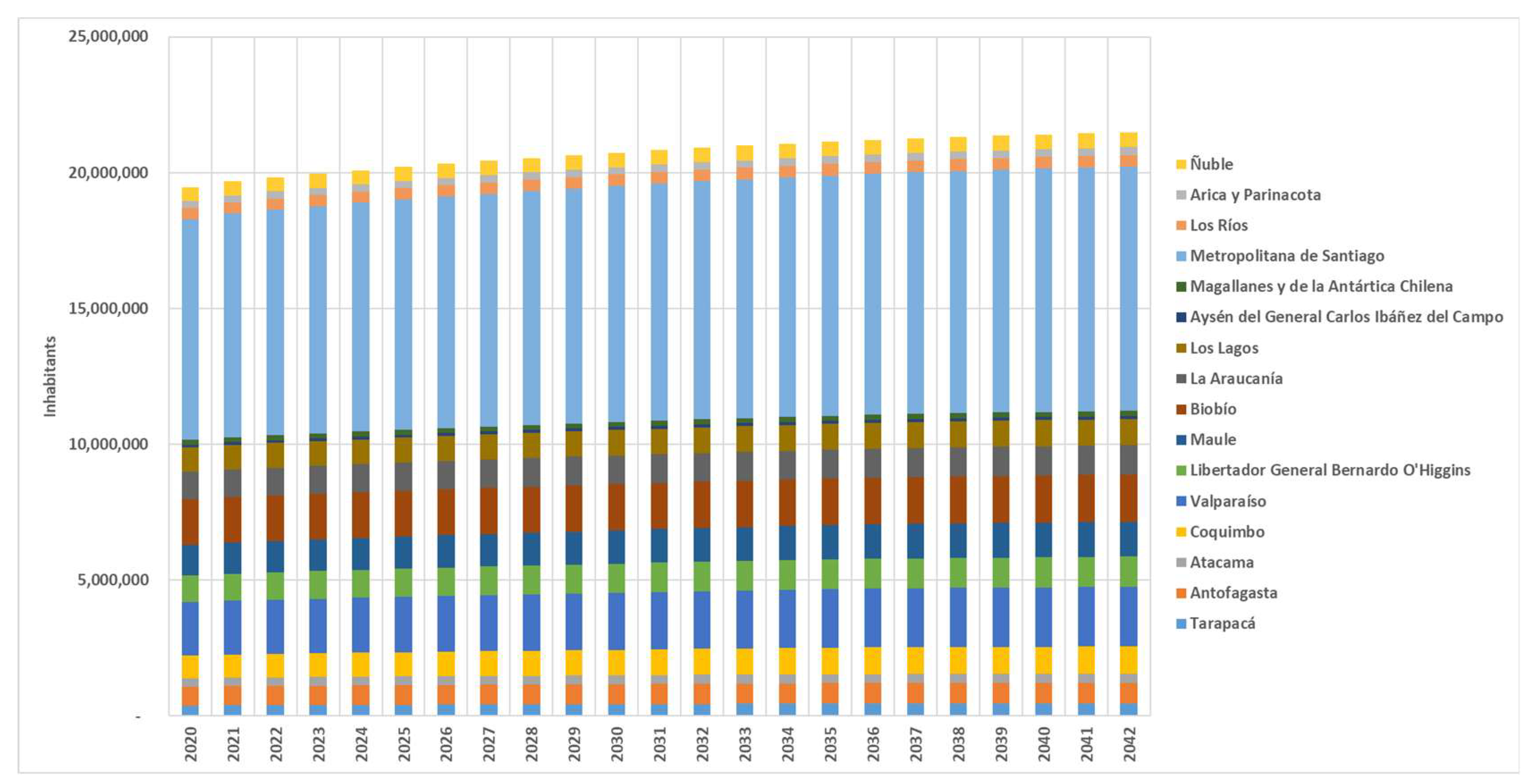
In the case of the population, the National Institute of Statistics carries out estimates and projections to the year 2035, by district and urban and rural area, which are extrapolated from the INE’s national projection to 2050. The following Figure 10 summarizes this projection to the year 2042, by region.

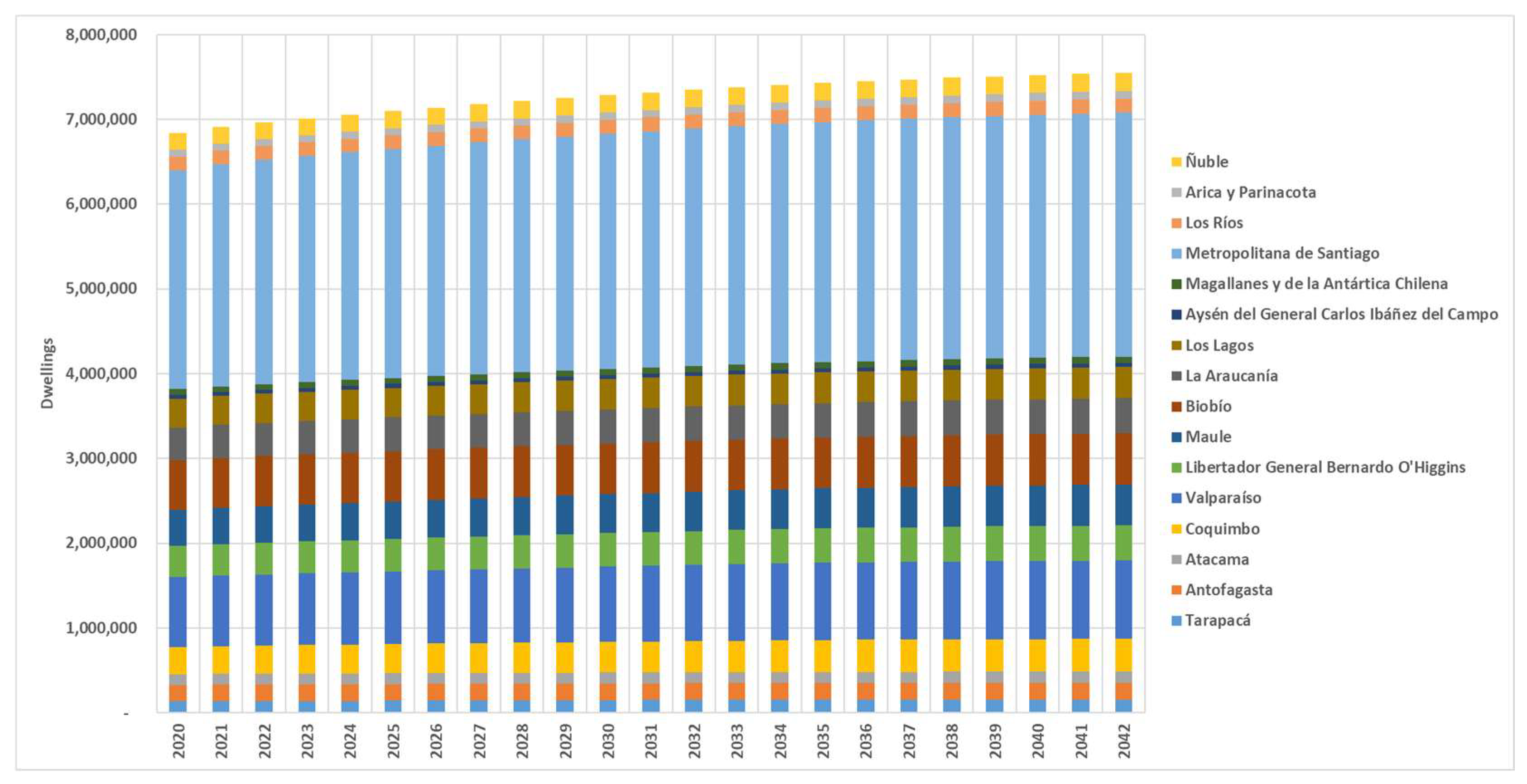
Based on the population projection, an estimate of the number of dwellings in the year 2042 is conducted. For this, housing data from the 2017 Census are used, as well as the projection of inhabitants per dwelling that has been estimated for Chile in previous studies [31]. Such studies project a rate of two inhabitants per dwelling to the year 2050, resulting in an increase in the number of dwellings based on this rate and the number of inhabitants per district. Figure 11 shows the projection of the national number of dwellings disaggregated by regions.

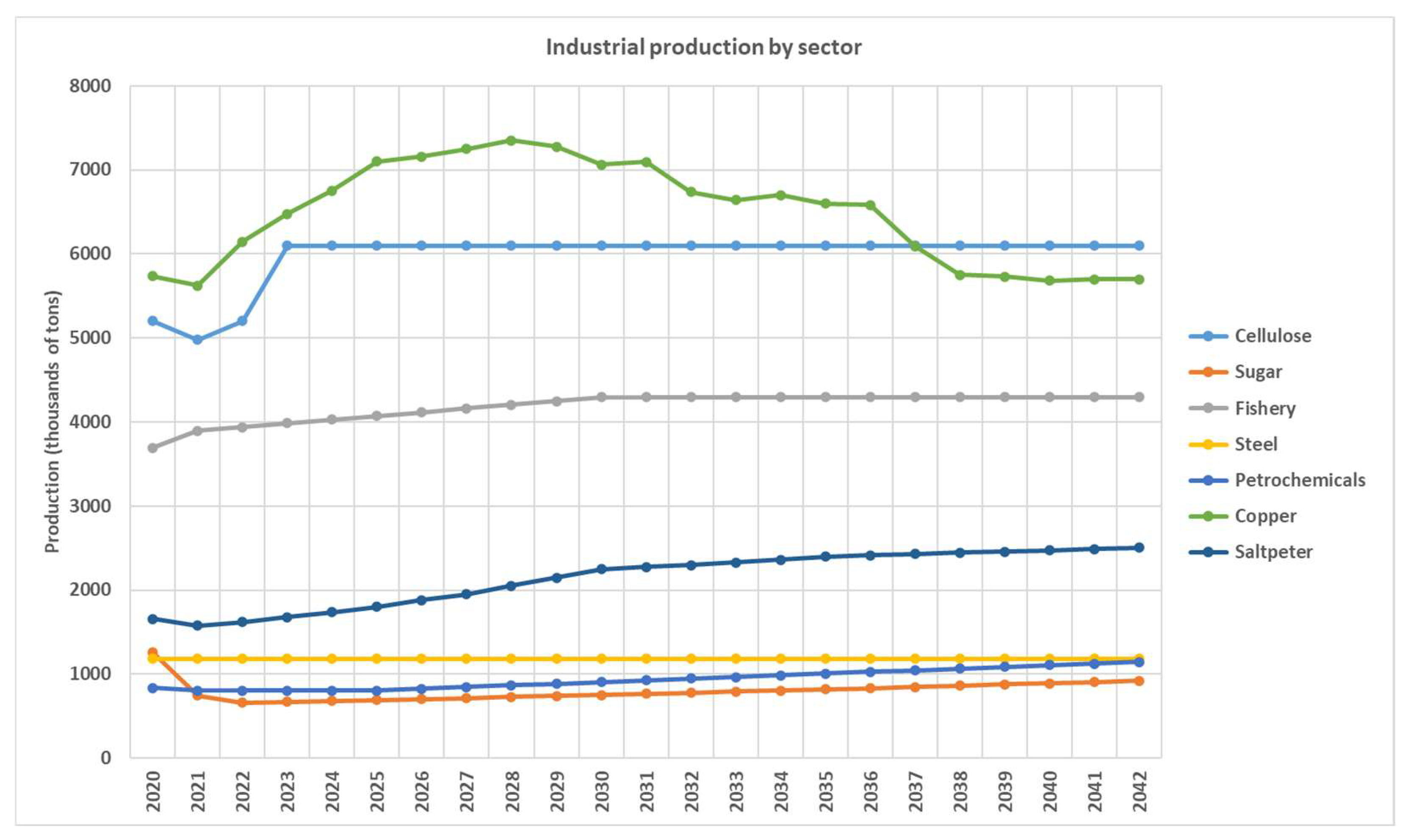
For cooper mining and other industrial sectors, the main driver to project the electric demand is the industrial projection. The copper ore processing for each mining company is used as input for the copper-mining industries electric demand model. For other industries, the industrial production projection is used as input (for example, steel production is used for the steel sector, cellulose production for paper and cellulose, and so on). The following sources of information were used to project the industrial production for each sector:

▪

Projected copper production per mine site from [25], additional information from this institution and Mining Policy 2050 (2021);

▪

Pulp and paper production based on increased installed capacity (MAPA project);

▪

Sugar production based on improved crop yields;

▪

Fishery production with an increase in fishery and aquaculture production of 15% by 2030, based on FAO and OECD statistics;

▪

Steel production is not expected to increase;

▪

Petrochemical production is expected to increase in e-methanol production by 2030, due to the green hydrogen impulse;

▪

Saltpeter production expects an increase in lithium production of 250 thousand tons per year and a potassium production of 2 million tons per year by 2030 [32].

Figure 12 shows the industrial production projection. It is important to highlight the significant drop in copper production that would occur due to the delay in the achievement of Codelco’s strategic projects and the lack of new projects on the country’s production horizon.

4. Results

Combining the estimations provided by the models described in the methodology sections (econometric models, end-use models, and exogenous projections), we forecast the net electric demand for Chile until 2041 for each major economic sector considering national, regional and bus spatial resolution. Two scenarios are evaluated: the base case scenario and a low-carbon emission scenario. In the base case scenario, it is supposed that there are no significant changes in the use of new technologies that could affect the projection of electricity demand. In the low-carbon emission scenario, an increase in electricity demand due to the widespread electrification measure is projected. To project the increase in electricity demand due to the widespread electrification, some measures included in the updated Nationally Determined Contribution (NDC) are taken as a reference. The following policies are included in the low carbon emission scenario:

▪

Electric heating: there will be a 57% and 70% share of electricity in homes and apartments for heating by 2050, respectively; the proportional replacement of other energy sources is considered, assuming a comfortably heated house;

▪

SMDG: there will be 4151 MW of installed capacity by the year 2042;

▪

Net billing: there will be 577 MW of distributed capacity by 2042 in the residential sector, and 2999 MW in the commercial sector;

▪

Electric vehicles: the measure corresponds to a gradual increase in the share of electric vehicles in total light vehicle sales, reaching 60% by 2040 (50% BEV and 10% PHEV). Also, 33% of the urban bus fleet corresponds to electric buses by 2040;

▪

Cooking: there will be a 15% share of energy demand for cooking with electricity by the year 2042;

▪

Air conditioning: 15% of homes will have access to air conditioning by the year 2042.

In the base case scenario, the effect of existing electric vehicles and buses, net billing projects and installed SMGD remains constant, as they are implicit in the historical net demand.

Regarding end uses in the residential sector, the base case corresponds to a constant share of electricity in the different uses, with demand growth only because of the number of dwellings. Therefore, the effect of end uses on the demand projection only considers the difference in electricity demand between the base scenario and the low-carbon emission scenario.

4.1. Base Case Scenario

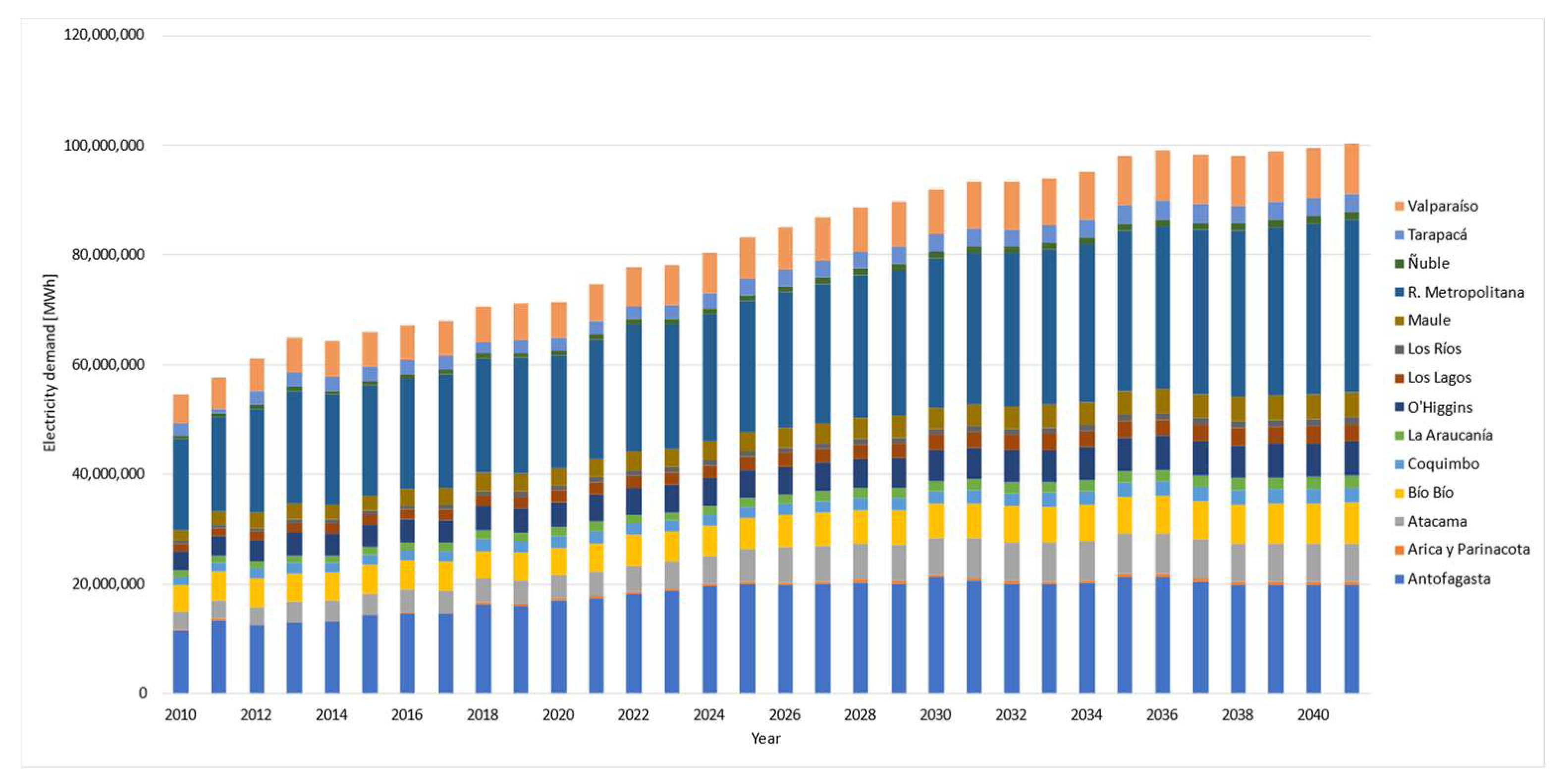
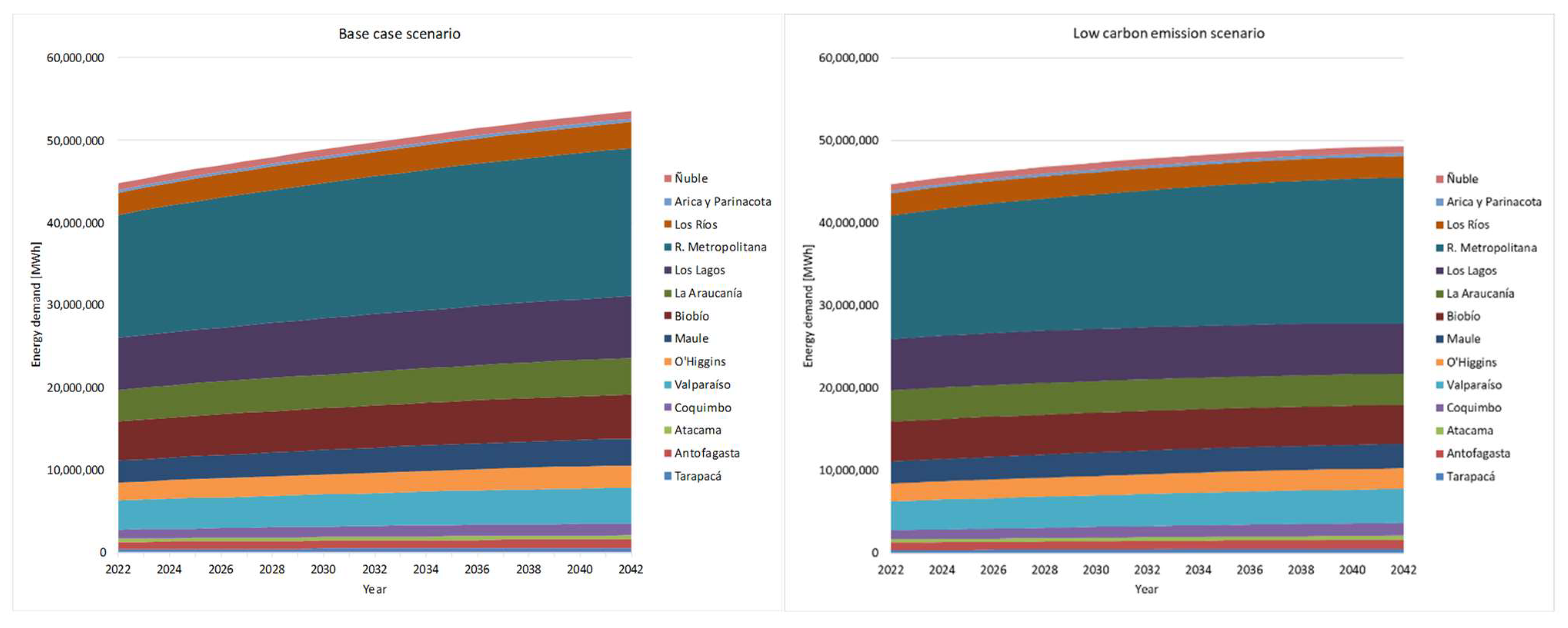
Figure 13 shows the electricity demand projection for each region that is part of the National Electric System for the base case scenario. In the next section, the low-carbon emission scenario results are compared regarding this base case scenario.

4.2. Low Carbon Emission Scenario

The low carbon emission scenario targets have a significant impact on the evolution of the generation and energy demand matrix. The following are some of the most representative.

4.2.1. Electricity Demand for Heating

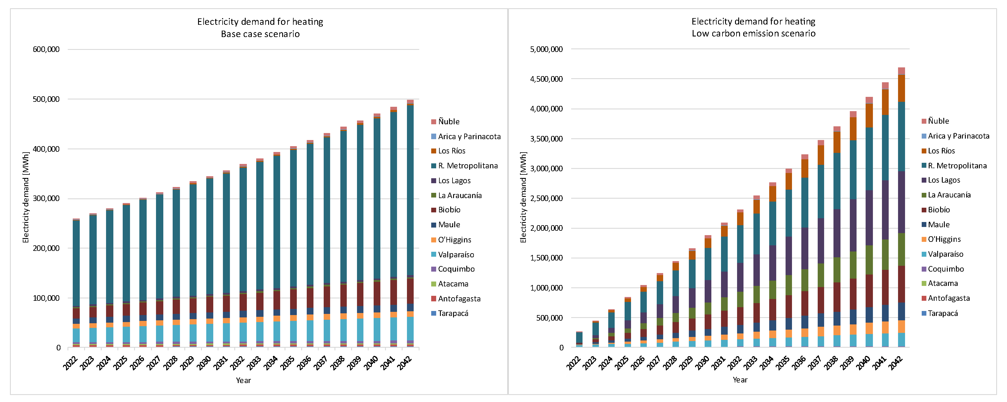
Figure 14 shows the projection of the electricity demand for heating for the low-carbon emission scenario compared to the base case scenario. An increase in electricity demand of 4189 GWh/year by 2042 is estimated in comparison to the base case scenario, highlighting its effect on regions that originally used other energy sources for heating (biomass or wood, liquefied gas, natural gas, and kerosene).

4.2.2. Electromobility

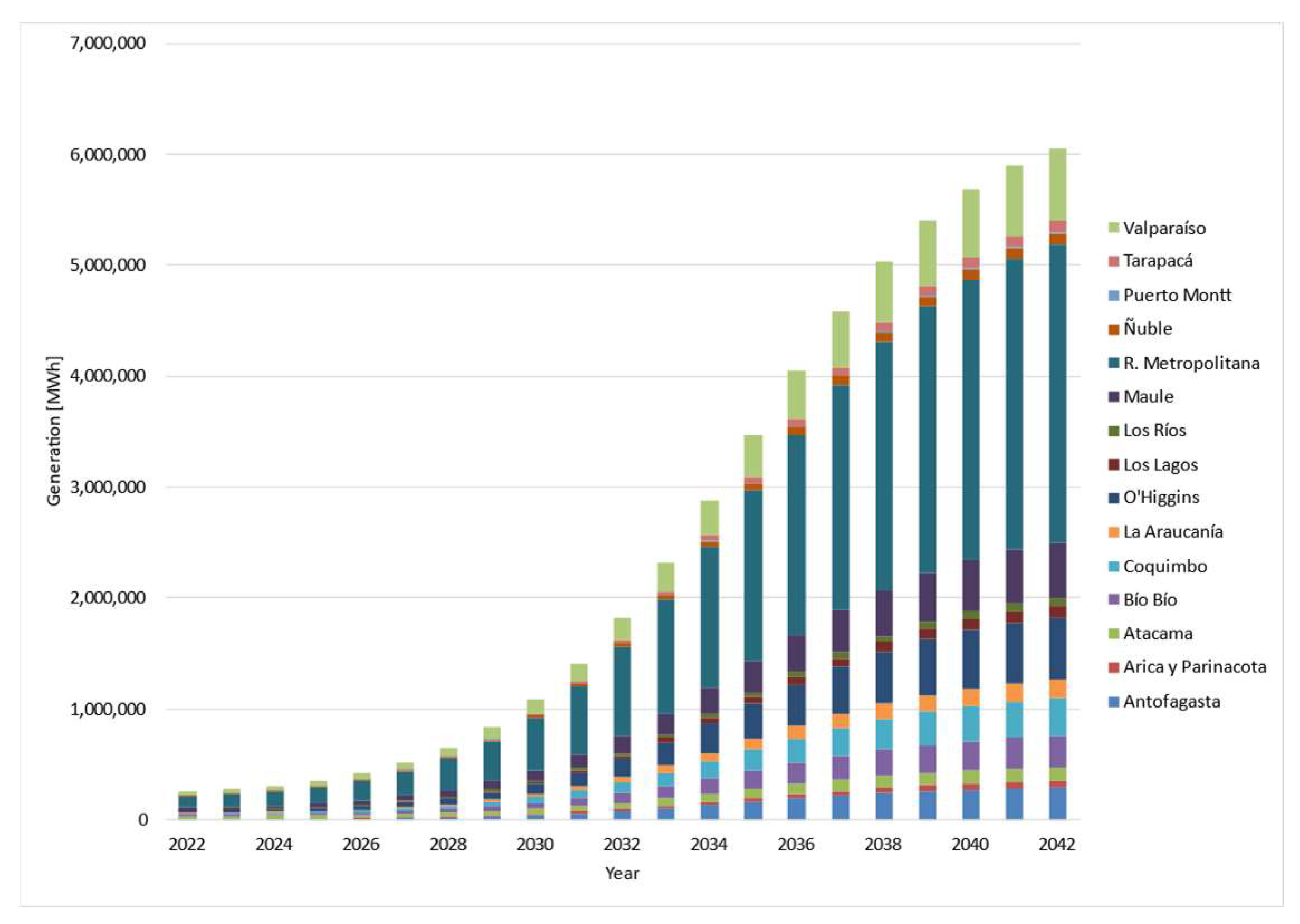
The electric demand resulting from the electromobility of the low-carbon scenario is presented in Figure 15. An increase in the electricity demand of 6014 GWh/year by 2042 is estimated in comparison to the base case scenario.

4.2.3. Net Billing and SMDG

The generation of net billing projects is presented in Figure 16. A decrease of 6054 GWh/year in the total demand by 2042 is estimated due to the introduction of net billing projects.

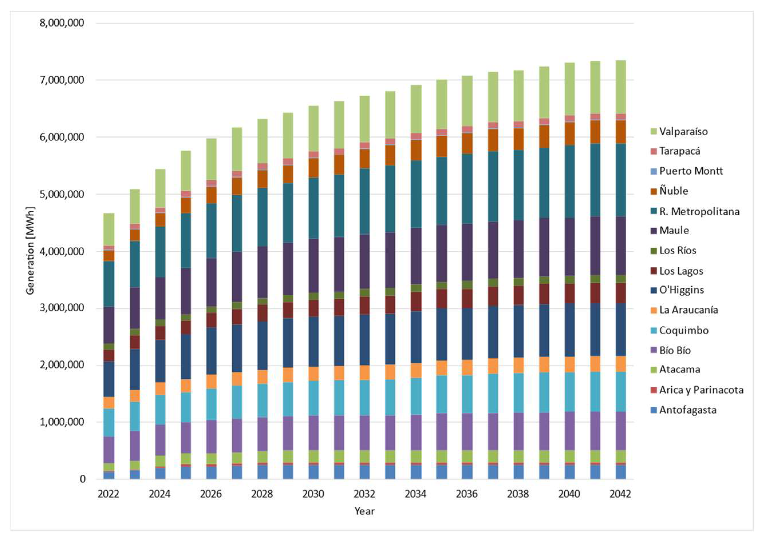
The generation of SMGD is presented in Figure 17. A decrease of 7346 GWh/year in the total demand is estimated by 2042.

4.2.4. Electricity Demand for Air Conditioning

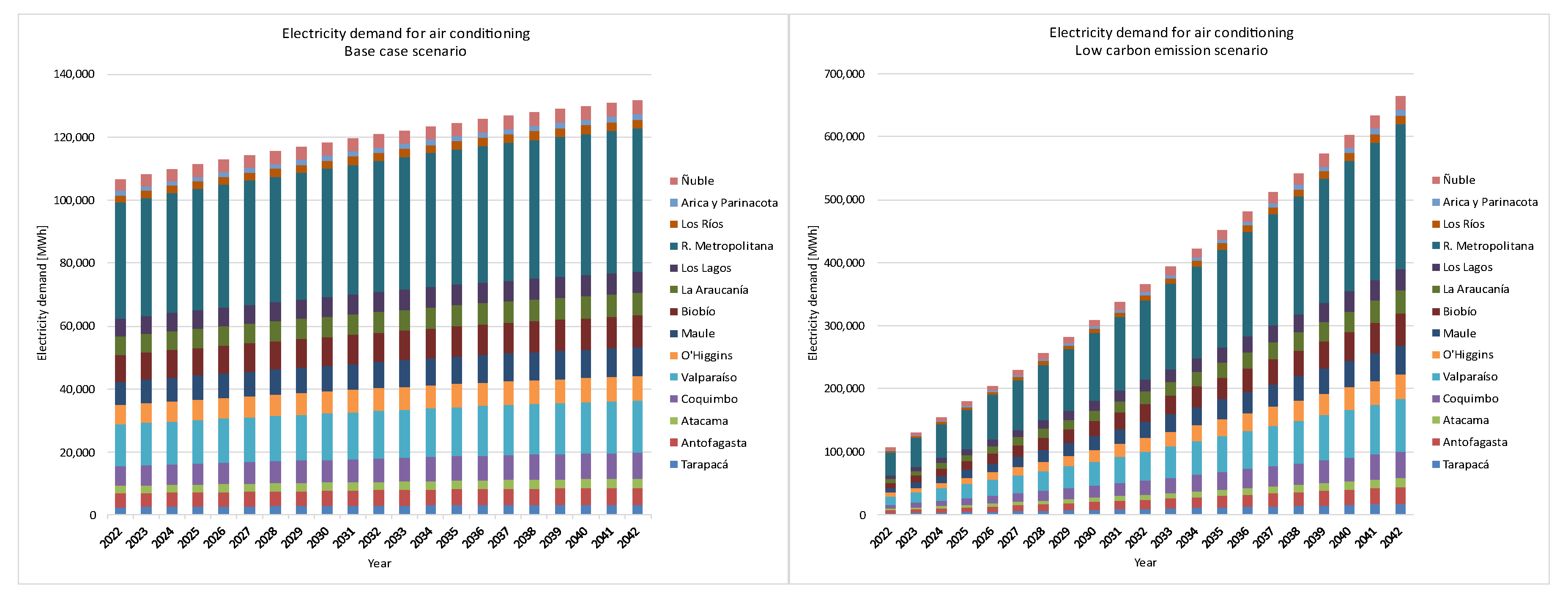
Figure 18 shows the electric demand for air conditioning, with an increase of 13% in access to air conditioning by 2042, compared to 3% in the base scenario; there is an increase in electricity demand of 533 GWh/year.

4.2.5. Energy Demand for Residential Sector

Figure 19 projects the annual total energy for the residential sector at the regional level, which includes all types of fuels, such as biomass, natural gas, kerosene, and electricity. Due to the implementation of mitigation action in the energy sector, the total energy demand by 2042 decreases by 4145 GWh, but the electric demand will increase by 6856 GWh.

4.2.6. Projection of the Net Electricity Demand

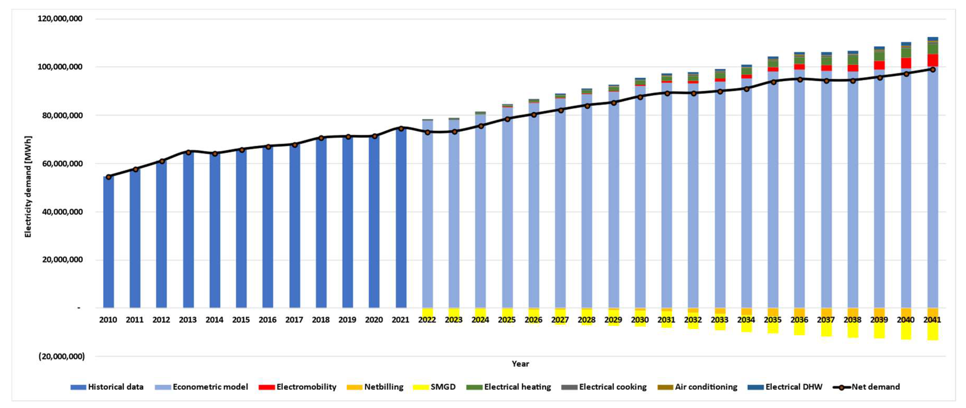
The final projection is shown in Figure 20. The blue bars depict historical data at national level, while light blue bars represent the aggregated projections derived from econometrics models. The green bars represent the effect of electrification in the residential sector, and red bars represent the electrical demand of electromobility projections. Negative values are depicted by yellow and light orange bars, representing the projections associated with SMGD and net billing projects, respectively. Finally, the black line illustrates the net electrical demand.

The result of this paper shows that the forecast of electric demand for Chile in 2041 is about 100.4 TWh/year; for comparison, the electric demand in 2021 was 74.8 TWh/yr. It is expected that electric demand due to electromobility in 2041 will be about 5.1 TWh/year; electrification in the residential sector due to low-carbon emission policies is expected to be about 6.8 TWh/year in 2041. The demand due to distributed generation is expected to be about −5.9 TWh in net billing projects and −7.3 TWh/year due to SMGD projects. Adding all of these up, the net electrical demand for Chile is forecast to be about 99.1 TWh/year in 20 years from today.

When splitting electrical demand into economic sectors at the national level, we can observe the significance of both the regulated sector and the non-regulated sector in distribution areas compared to the total demand. Sub-sectors such as residential, commercial, public sector, and minor industries are included in the demand of distribution areas, represented by the grey area in Figure 21. The copper-mining industry, highlighted in yellow, accounts for nearly a third of Chilean electricity demand. Other relevant economic sectors are other mining industries, paper and cellulose, cement, and steel, among others. It is expected that the regulated sector will keep growing as long as economic growth is increasing too. At the same time, copper demand depends on the development of new mining projects, while the increasing electric demand for existing mining projects can be attributed to efficiency losses due to the decrease in copper ore grade.

The results shown above, at the national level, were also estimated at the bus level for the Chilean electrical grid at monthly resolution and for every economic sector. Figure 22 and Figure 23 (see below) present some projections for buses located in northern and central–southern Chile. The DEMPRO-GIS software, developed as part of this study, enables the forecasting of electrical demand at every bus in the Chilean grid with its georeferenced location. This tool assists the Coordinator in identifying varied growth rates at each location in Chile. For instance, in the northern part of Chile, most of the electrical demand stems from copper-mining industries, while the southern regions exhibit significant residential heating energy consumption, offering substantial potential for electrification initiatives.

5. Conclusions

This paper presents a methodology developed and applied to forecast electrical demand for the Chilean Electrical Power System. The forecast considers national, regional, district and bus spatial disaggregation for the period 2022–2042. In comparison with previous studies, the proposed methodology allows for the projection of the electric demand with bus spatial disaggregation. Using econometric and end-use models, it was possible to forecast the demand considering the impact of low-carbon emission technologies, which the current energy policy in Chile promotes to achieve carbon neutrality by 2050. In the base case scenario, it is projected that electric demand in 2042 will be 100,352 GWh, and due to the massification of the low-carbon emission technologies, the electric demand will be 112,358 GWh. However, due to the introduction of distributed generation (net billing and SMDG), it is expected that the net demand will be 99,119 GWh.

References

1. Ghods, L.; Kalantar, M. Different Methods of Long-Term Electric Load Demand Forecasting; A Comprehensive Review. Iran. J. Electr. Electron. Eng. 2011, 7, 249–259. [Google Scholar]
2. Ahmad, N.; Ieee, M.; Ghadi, Y.; Ieee, S.M.; Adnan, M. Load Forecasting Techniques for Power System: Research Challenges and Survey. IEEE Access 2022, 10, 71054–71090. [Google Scholar] [CrossRef]
3. Mystakidis, A.; Koukaras, P.; Tsalikidis, N.; Ioannidis, D.; Tjortjis, C. Energy Forecasting: A Comprehensive Review of Techniques and Technologies. Energies 2024, 17, 1662. [Google Scholar] [CrossRef]
4. Ha, S.; Tae, S.; Kim, R. Energy Demand Forecast Models for Commercial Buildings in South Korea. Energies 2019, 12, 2313. [Google Scholar] [CrossRef]
5. Agrawal, R.K.; Muchahary, F.; Tripathi, M.M. Long Term Load Forecasting with Hourly Predictions Based on Long-Short-Term-Memory Networks. In Proceedings of the 2018 IEEE Texas Power and Energy Conference, TPEC 2018, College Station, TX, USA, 8–9 February 2018. [Google Scholar] [CrossRef]
6. Gebremeskel, D.H.; Ahlgren, E.O.; Beyene, G.B. Long-Term Evolution of Energy and Electricity Demand Forecasting: The Case of Ethiopia. Energy Strategy Rev. 2021, 36, 100671. [Google Scholar] [CrossRef]
7. Li, J.; Luo, Y.; Wei, S. Long-Term Electricity Consumption Forecasting Method Based on System Dynamics under the Carbon-Neutral Target. Energy 2022, 244, 122572. [Google Scholar] [CrossRef]
8. Jiménez, J.; Pertuz, A.; Quintero, C.G.; Montaña, J. Multivariate Statistical Analysis Based Methodology for Long-Term Demand Forecasting. IEEE Lat. Am. Trans. 2019, 17, 93–101. [Google Scholar] [CrossRef]
9. Velasquez, C.E.; Zocatelli, M.; Estanislau, F.B.G.L.; Castro, V.F. Analysis of Time Series Models for Brazilian Electricity Demand Forecasting. Energy 2022, 247, 123483. [Google Scholar] [CrossRef]
10. Rizzati, M.; De Cian, E.; Guastella, G.; Mistry, M.N.; Pareglio, S. Residential Electricity Demand Projections for Italy: A Spatial Downscaling Approach. Energy Policy 2022, 160, 112639. [Google Scholar] [CrossRef]
11. Zhang, C.; Mauleón, I. Assessing the Energy Efficiency Gains and Savings in China’s 2060 Carbon-Neutral Plan. Energies 2023, 16, 6863. [Google Scholar] [CrossRef]
12. Zhou, K.; Chu, Y.; Hu, R. Energy Supply-Demand Interaction Model Integrating Uncertainty Forecasting and Peer-to-Peer Energy Trading. Energy 2023, 285, 129436. [Google Scholar] [CrossRef]
13. Pesantez, J.E.; Li, B.; Lee, C.; Zhao, Z.; Butala, M.; Stillwell, A.S. A Comparison Study of Predictive Models for Electricity Demand in a Diverse Urban Environment. Energy 2023, 283, 129142. [Google Scholar] [CrossRef]
14. Jin, H.; Guo, J.; Tang, L.; Du, P. Long-Term Electricity Demand Forecasting under Low-Carbon Energy Transition: Based on the Bidirectional Feedback between Power Demand and Generation Mix. Energy 2024, 286, 129435. [Google Scholar] [CrossRef]
15. Bashiri Behmiri, N.; Fezzi, C.; Ravazzolo, F. Incorporating Air Temperature into Mid-Term Electricity Load Forecasting Models Using Time-Series Regressions and Neural Networks. Energy 2023, 278, 127831. [Google Scholar] [CrossRef]
16. Luzia, R.; Rubio, L.; Velasquez, C.E. Sensitivity Analysis for Forecasting Brazilian Electricity Demand Using Artificial Neural Networks and Hybrid Models Based on Autoregressive Integrated Moving Average. Energy 2023, 274, 127365. [Google Scholar] [CrossRef]
17. Bodong, S.; Wiseong, J.; Chengmeng, L.; Khakichi, A. Economic Management and Planning Based on a Probabilistic Model in a Multi-Energy Market in the Presence of Renewable Energy Sources with a Demand-Side Management Program. Energy 2023, 269, 126549. [Google Scholar] [CrossRef]
18. Hamed, M.M.; Ali, H.; Abdelal, Q. Forecasting Annual Electric Power Consumption Using a Random Parameters Model with Heterogeneity in Means and Variances. Energy 2022, 255, 124510. [Google Scholar] [CrossRef]
19. Wu, W.Z.; Pang, H.; Zheng, C.; Xie, W.; Liu, C. Predictive Analysis of Quarterly Electricity Consumption via a Novel Seasonal Fractional Nonhomogeneous Discrete Grey Model: A Case of Hubei in China. Energy 2021, 229, 120714. [Google Scholar] [CrossRef]
20. Zhao, Z.; Zhang, Y.; Yang, Y.; Yuan, S. Load Forecasting via Grey Model-Least Squares Support Vector Machine Model and Spatial-Temporal Distribution of Electric Consumption Intensity. Energy 2022, 255, 124468. [Google Scholar] [CrossRef]
21. Kazemzadeh, M.R.; Amjadian, A.; Amraee, T. A Hybrid Data Mining Driven Algorithm for Long Term Electric Peak Load and Energy Demand Forecasting. Energy 2020, 204, 117948. [Google Scholar] [CrossRef]
22. Coordinador Eléctrico de Estudio. Proyección de Demanda Eléctrica 2019–2039; Coordinador Eléctrico de Estudio: Santiago, Chile, 2018. [Google Scholar]
23. Ministerio de Energía. Planificación Energética de Largo Plazo. Informe Preliminar; Ministerio de Energía: Santiago, Chile, 2021. [Google Scholar]
24. Comisión Nacional de Energía. Informe Definitivo de Previsión de Demanda 2021–2041; Comisión Nacional de Energía: Santiago, Chile, 2022. [Google Scholar]
25. COCHILCO. Proyección Del Consumo de Energía Eléctrica En La Minería Del Cobre 2021–2032; COCHILCO: Santiago, Chile, 2022. [Google Scholar]
26. Valgesta Energía. Estudio de Previsión de Demanda Eléctrica Regulada 2021–2041; Asociación Gremial Empresas Eléctricas: Santiago, Chile, 2021. [Google Scholar]
27. Ministerio de Energía. Gobierno de Chile. Carbono Neutralidad en el Sector Energía. Proyección de Consumo Energético Nacional 2020; Ministerio de Energía: Santiago, Chile, 2020. [Google Scholar]
28. Ministerio de Energía. Proceso de Planificación Energética de Largo Plazo. Informe Final Corregido 2018; Ministerio de Energía: Santiago, Chile, 2018. [Google Scholar]
29. Centro de Energía FCFM Universidad de Chile. Actualización Metodológica Del Modelo de Consumo Energético y Emisiones Para El Sector Transporte (STEP) Etapa II; Ministerio de Transporte y Telecomunicaciones: Santiago, Chile, 2022. [Google Scholar]
30. CDT. Informe Final de Usos de La Energía de Los Hogares de Chile; CDT: Santiago, Chile, 2018. [Google Scholar]
31. Centro de Energía FCFM Universidad de Chile. Estudio de Actualización y Complementación de Herramientas de Prospectiva de Largo Plazo Asociadas a La Demanda Energética; Centro de Energía: Santiago, Chile, 2019. [Google Scholar]
32. Servicio Nacional de Geología y Minería. Anuario de La Minería de Chile 2018; Servicio Nacional de Geología y Minería: Santiago, Chile, 2018. [Google Scholar]
Figure 1. The red points represent the geographical location of some buses in the Electric National System of Chile. The blue, green, and black lines represent transmission lines in different voltage levels.
Energies 17 03448 g001
Figure 2. Electric demand organized by type of clients, where “R” is regulated clients, L is “non-regulated clients”, and “L_D” represents non-regulated clients connected to the distribution power system.
Energies 17 03448 g002
Figure 3. Methodology used to project electrical demand.
Energies 17 03448 g003
Figure 4. Historical generation of SMDG power plants by technology.
Energies 17 03448 g004
Figure 5. Historical generation of SMDG power plants by region.
Energies 17 03448 g005
Figure 6. Estimated historical generation of Net billing projects, by region.
Energies 17 03448 g006
Figure 7. Effect of distributed generation on the estimation of real electricity demand.
Energies 17 03448 g007
Figure 8. Methodological diagram of the cross-referencing of the information and variables used in the end-use model.
Energies 17 03448 g008
Figure 9. IMACEC historical and projection.
Energies 17 03448 g009
Figure 10. National population projection disaggregated by region (1 to 16).
Energies 17 03448 g010
Figure 11. Projection of the national number of dwellings disaggregated by regions (1 to 16).
Energies 17 03448 g011
Figure 12. Industrial production projections.
Energies 17 03448 g012
Figure 13. Annual electricity demand by regions, baseline scenario.
Energies 17 03448 g013
Figure 14. Annual electricity demand for final use in heating by region, base case (left) and low-carbon emission scenario (right).
Energies 17 03448 g014
Figure 15. Annual electricity demand for electromobility by regions.
Energies 17 03448 g015
Figure 16. Annual generation of residential and commercial net billing projects.
Energies 17 03448 g016
Figure 17. Annual energy generated from SMDG projects by regions.
Energies 17 03448 g017
Figure 18. Annual electricity demand for air conditioning end use by regions, base case (left) and low-carbon emission scenario (right).
Energies 17 03448 g018
Figure 19. Annual energy demand by regions, baseline (left) and low carbon emission (right) scenario.
Energies 17 03448 g019
Figure 20. Projected electricity demand for Chile, including econometric models, end-use models, and exogenous projections.
Energies 17 03448 g020
Figure 21. Projected electricity demand for Chile by economic sector.
Energies 17 03448 g021
Figure 22. Monthly electricity withdrawals for Cardones 220 kV bus by a copper-mining company in the north of Chile, historical data (2010–2021) and projection (2022–2041). The blue, green, and orange lines represent transmission lines in different voltage levels.
Energies 17 03448 g022
Figure 23. Monthly electricity withdrawals for Macul 12 kV bus in the city of Santiago, historical data (2010–2021) and projection (2022–2041). The blue, green, and orange lines represent transmission lines in different voltage levels.
Energies 17 03448 g023