Building a Sustainable Future: A Three-Stage Risk Management Model for High-Permeability Power Grid Engineering

Abstract

Under the background of carbon neutrality, it is important to construct a large number of high-permeability power grid engineering (HPGE) systems, since these can aid in addressing the security and stability challenges brought about by the high proportion of renewable energy. Construction and engineering frequently involve multiple risk considerations. In this study, we constructed a three-stage comprehensive risk management model of HPGE, which can help to overcome the issues of redundant risk indicators, imprecise risk assessment techniques, and irrational risk warning models in existing studies. First, we use the fuzzy Delphi model to identify the key risk indicators of HPGE. Then, the Bayesian best–worst method (Bayesian BWM) is adopted, as well as the measurement alternatives and ranking according to the compromise solution (MARCOS) approach, to evaluate the comprehensive risks of projects; these methods are proven to have more reliable weighting results and a larger sample separation through comparative analysis. Finally, we established an early warning risk model on the basis of the non-compensation principle, which can help prevent the issue of actual risk warning outcomes from being obscured by some indicators. The results show that the construction of the new power system and clean energy consumption policy are the key risk factors affecting HPGE. It was found that four projects are in an extremely high-risk warning state, five are in a relatively high-risk warning state, and one is in a medium-risk warning state. Therefore, it is necessary to strengthen the risk prevention of HPGE and to develop a reasonable closed-loop risk control mechanism.

1. Introduction

The emission of greenhouse gases is one of the most prevalent reasons for global warming; according to the World Resources Institute (WRI), carbon dioxide accounts for 77% of all greenhouse gas emissions (World Resources Institute (WRI): https://www.wri.org/). In order to solve the increasingly severe climate change issues and to reduce carbon emissions, various countries have put forward corresponding climate policies. So far, nearly 150 countries and regions have proposed the climate target of “zero carbon” or being “carbon neutral” [1]. As one of the major carbon-emitting countries [2], China has committed to achieving its peak carbon dioxide emissions before 2030 and to bring about carbon neutrality before 2060.

The carbon emissions of the power sector—one of the largest carbon emitters—account for over 40% of China’s emissions [3]. Hence, it is necessary to accelerate the transformation of energy structures and to adjust the energy consumption of the power industry. On 15 March 2021, China proposed the formation of a new power system that is dominated by renewable energy (wind power and photovoltaics) [4]. Under this target, it is suggested that the proportion of non-fossil fuel energy consumption will be at 25% by 2030 and that the proportion of non-fossil fuel energy consumption will be at 80% by 2060 (Central People’s Government of the People’s Republic of China (CPGPRC): http://www.gov.cn). However, high-permeability renewable energy will impact the safe and stable operation of the power system [5]; this also brings about new challenges in the establishment and development of new power systems.

High-permeability power grid engineering (HPGE) is a typical power grid project (PGP) that satisfies the safety, intelligence, and flexibility requirements through the construction of lines, transformers, intelligent control systems, and energy storage devices. On the one hand, resource waste can be prevented and the absorption capacity of renewable energy can be increased through the development of HPGE. On the other hand, it can also increase the effectiveness of the power system’s operation and guard against damage to the electrical equipment and power grid.

However, various risks such as those relating to cost, policy, and social factors will arise during the design, building, and operation processes [6,7,8]. Similarly, HPGE also faces the challenges of intricate internal and external hazards. As the matter stands, value-at-risk (VaR) and optimization algorithms are widely used for risk measurement [9,10,11]. However, these models emphasize the single risk of PGPs and are less able to achieve a multi-dimensional risk collaborative assessment. Thus, thorough risk management is required for HPGE, which can also help to provide closed-loop control over risk identification, assessment, and early warning.

2. Literature Review

Risk management has always been a research hotspot for scholars; common methods of this technique mainly include the VaR approach, optimization algorithms, and the multi-criteria decision-making (MCDM) theory. Among them, the former mainly focuses on the measurement of financial risks in the investment process [12], while the latter focuses more on the comprehensive risk assessment of the evaluation object [13]. Risk management based on MCDM mainly includes the following parts:

➢

Risk identification

Risk identification refers to the first step of risk management. Accurate risk identification is conducive to subsequent risk assessment and risk warning. Zhou et al. established a two-layer neural network risk identification model, which considered the multi-attributes of indicators [14]. Through the proposed risk identification model, the accuracy of subsequent risk calculation results was significantly improved. Rao et al. identified 222 schedule risks of power grid engineering projects through questionnaires and expert interviews [15]. Meanwhile, Zhang et al. used the system dynamics (SD) approach to identify risks in the engineering environment, which can also help in the identification of the interactions among different risk factors [16]. Wang et al. established a railway project construction safety risk identification model based on the work breakdown structure and risk breakdown structure approaches [17].

➢

Risk assessment

On the basis of the risk identification process, it is essential to further evaluate the comprehensive risks faced by the project. Risk assessments based on MCDM mainly include two parts—one is indicator weighting, and the other is the comprehensive assessment of the object to be assessed. The commonly used MCDM models in engineering risk assessment are shown in

Table 1. The commonly used MCDM models in engineering risk assessment.

Type	Sub-Type	Model	Characteristics
Weighting method	Subjective	Analytic hierarchy process (AHP) [18]	The operation is simple, but the indicators need to be compared in pairs.
		Analytic network process (ANP) [19]	ANP considers the interaction between factors or adjacent levels.
		Best–worst method (BWM) [20]	BWM is more convenient and efficient due to the fewer index comparisons.
	Objective	Entropy weight method (EWM) [21]	EWM determines the index weight according to the information entropy.
		Coefficient of variation (CV) [22]	CV gives weight to indicators according to their dispersion.
Evaluation approach	Ranking	CRITIC method [23]	CRITIC simultaneously considers the conflict and comparative strength of indicators.
		TOPSIS method [24]	TOPSIS eliminates the impact of different indicator dimensions but ignores the ideal solution.
		VIKOR method [25]	VIKOR can obtain a compromise scheme with priority but requires certain criteria values.
	Rating/Grading	Gray relation analysis (GRA) [26]	GRA has no strict requirements on sample richness and regularity.
		Matter-element extension model (MEEM) [27]	MEEM can conduct evaluation research even if there is only one evaluation object.

.

As concerns index weighting, there are mainly two types of weighting methods. The first type is that of objective weighting methods, which mainly measure the inter-group differences and dispersion between indicators through quantitative means so as to achieve the weight assignment of each indicator. The second type is that of subjective weighting methods, which are mainly based on expert experience to determine the weight. Although the former can avoid the subjectivity and limitations brought about by the subjective weighting method to a certain extent, it has high requirements for data capacity and sample richness.

As concerns scheme evaluation, the rating/grading models mainly assess the risk level of a single project (such as bad, medium, and good), while the ranking models focus more on the comparison and risk ranking of multiple evaluation objects.

➢

Early risk warning

As a supplement to risk assessment, early risk warning is also an essential process in risk management. The current research on early risk warning is mostly qualitative, which means that the targeted measures and suggestions are put forward as risk responses according to the risk assessment results. When the research object is time series data, some scholars also use machine learning methods for engineering early risk warning. Deng constructed an early risk warning model for engineering based on the BP neural network [28]. He et al. proposed a WOE-GA-BP model to determine geological disaster early risk warnings [29]. The above risk warning research is essentially a prediction of the future project warning situation. In addition, when the research object is a static sample, most studies mainly set a certain early risk warning threshold to achieve a comprehensive early warning of engineering risks [30]; this is the early risk warning processing method used in this paper.

Through a summary of the existing literature, we found that most of the current PGP risk research is only carried out from the viewpoint of one of the three dimensions mentioned above. Few studies have built a relatively complete and comprehensive risk management system for PGPs. As the matter stands, the existing research on the risk management of PGPs focuses more on traditional power transmission projects or ultra-high voltage projects; there is a gap in risk management research for HPGE. Against this background, this paper innovatively proposes a comprehensive risk management model that is applicable to HPGE. The innovations and contributions are as follows:

➢

This paper constructs a risk evaluation index system for HPGE from the following four dimensions: policy, finance, operation, and technical environment. The indicators are obtained through risk identification using the fuzzy Delphi method.

➢

A risk assessment model of a high-permeability PGP is established through the Bayesian best–worst method (Bayesian BWM), as well as the measurement alternatives and ranking according to the compromise solution (MARCOS) approach. The superiority of the applied models is verified by comparing them with the traditional BWM and TOPSIS methods.

➢

Considering the non-compensatory principle among primary indicators, an early risk warning model based on the multiplicative synthesis technique is proposed in this paper.

3. Methodology and Research Framework

3.1. Fuzzy Delphi for Risk Identification

The Delphi method was first proposed by Dalky and Helmer in 1963, and it can integrate the opinions of various experts to achieve evaluation through anonymous voting [31]. The traditional Delphi method requires experts to carry out four rounds of consultations; however, repeated discussions will greatly waste time and decrease efficiency [32]. In addition, it is often difficult to obtain consistent results due to the different experiences of experts. In this paper, we introduced the fuzzy theory into the traditional Delphi method, forming the fuzzy Delphi method; this method can help to cope with the aforementioned problems. Through the use of the membership function instead of expert opinion, experts do not need to repeatedly revise their opinions [33]. Meanwhile, there is no loss of useful information, because all expert opinions are given via the membership function. The steps of the fuzzy Delphi method for risk identification are introduced as follows:

➢

Step 1: Questionnaire design.

The value range of the conservative value and optimistic value of each indicator should be determined by the experts. Usually, the value range is 0–10.

➢

Step 2: Construct the triangular fuzzy number (TFN)

Collect the maximum and minimum values of each indicator scored by experts, and calculate the geometric mean value. The conservative TFN $\left(C_L^i,C_M^i,C_U^i\right)$ and optimistic TFN $\left(O_L^i,O_M^i,O_U^i\right)$ of each indicator are constructed.

Of these, $C_L^i$, $C_U^i$ and $C_M^i$, respectively, represent the minimum conservative value, maximum conservative value, and the geometric mean of the conservative value of experts on the indicator $i$. Correspondingly, $O_L^i$, $O_U^i$ and $O_M^i$, respectively, represent the minimum optimistic value, maximum optimistic value, and geometric mean of the optimistic value of all experts on the indicator $i$.

➢

Step 3: Judge the consistency of each expert’s scoring, and calculate the indicator’s consistent significance value $G_i$.

(1) If $C_U^i\le O_L^i$, it indicates that the expert scoring of the indicator is consistent, and $G_i$ can be calculated as follows:

$$G_i=\frac{C_M^i+O_M^i}{2}$$

(1)

(2) If $C_U^i>O_L^i$, the corresponding gray interval values $Z^i$ and $M^i$ need to be calculated as follows:

$$\{\begin{array}{l}{Z}^i=C_U^i-O_L^i\\ M^i=O_U^i-O_M^i\end{array}$$

(2)

If $M^i\ge Z^i$, $G_i$ can be obtained as follows:

$$G_i=\frac{[(C_U^i\times O_M^i)-(O_L^i\times C_M^i)]}{[(C_U^i-C_M^i)+(O_M^i-O_L^i)]}$$

(3)

If $M^i<Z^i$, it means that the evaluation of indicator $i$ by the experts is not consistent, and $G_i$ cannot be calculated. Hence, it is necessary to re-score the indicator and repeat the previous steps until the experts can converge on the evaluation of the indicator.

➢

Step 4: Filter indicators according to $G_i$.

Set the threshold of $G_i$, and compare the indicator’s consistent significance value of each indicator with the threshold. The indicators with values greater than the threshold value are retained, and the indicators with values less than the threshold value are discarded. In this paper, the threshold is set to 5.5.

3.2. Bayesian Best–Worst Method for Risk Indicator Weighting

Compared with the traditional AHP method, BWM can help decrease the comparison numbers between indicators [34]. However, it also faces outlier sensitivity and restricted information provision issues [35]. In 2019, Mohammadi and Rezaei combined the Bayesian theory and the traditional BWM method to form the Bayesian BWM approach, which can solve the aforementioned problems [36]. Considering the space limitation, the specific steps of the traditional BWM method will not be introduced; interested readers can consult Rezaei’s reference [37]. The basic steps of Bayesian BWM are given as follows:

➢

Step 1: Determine the best (most important) indicator $c_B$ and worst (least important) indicator $c_W$ for HPGE.

The best indicator means the risk factor that has the greatest impact on the HPGE, and the worst indicator means the risk factor that has the least impact on the HPGE.

➢

Step 2: Determine the “Best-to-Others (BO)” vector $A_B$ and the “Others-to-Worst (OW)” vector $A_W$.

Compare $c_B$ with other indicators $c_j$, and use 1 to 9 to represent the importance of $c_B$ with other indicators. The 1 means that the importance of $c_B$ and $c_j$ is equal, 9 means that $c_B$ is far more important than $c_j$. Similarly, compare $c_W$ with other indicators $c_j$, of which, 1 means that the importance of $c_W$ and $c_j$ is equal, and 9 means that the importance of $c_j$ is much higher than that of $c_W$. The BO and OW vectors can be expressed as follows:

$$\{\begin{array}{l}{A}_B=\left(a_{B1},a_{B2},\dots ,a_{Bn}\right)\\ A_W=\left(a_{1W},a_{2W},\dots ,a_{nW}\right)\end{array}$$

(4)

Through Equation (4), we can clearly understand the judgment results of various experts on the importance of various HPGE risk indicators.

➢

Step 3: Construct a multinomial probability distribution function.

Different from the traditional BWM, Bayesian BWM considers the probability interpretation of input and output. In other words, the indicators can be regarded as random events and the weights can be considered as the probability of events. Taking the worst indicator as an example, the multinomial probability distribution function of $c_W$ can be constructed as follows:

$$P\left(A_W|w\right)=\frac{\left({\displaystyle \sum _{j=1}^n{a}_{jW}}\right)!}{{\Pi }_{j=1}^n{a}_{jW}!}{\displaystyle \prod _{j=1}^n{w}_j^{a_{jW}}}$$

(5)

where $w$ represents the probability distribution.

➢

Step 4: Calculate the occurrence probability of indicators for HPGE.

The occurrence probability $w_j$ is positively correlated with the number of occurrences of the event $j$, which can be expressed as follows:

$$w_j\propto \frac{a_{jW}}{{\displaystyle \sum _{j=1}^n{a}_{jW}}}$$

(6)

Therefore, the probability of occurrence of $c_W$ can be expressed as follows:

$$w_{\mathrm{W}}\propto \frac{a_{\mathrm{WW}}}{{\displaystyle \sum _{j=1}^n{a}_{j\mathrm{W}}}}=\frac{1}{{\displaystyle \sum _{j=1}^n{a}_{j\mathrm{W}}}}$$

(7)

Then, it can be obtained through Equations (6) and (7), as follows:

$$\frac{w_j}{w_{\mathrm{W}}}\propto a_{j\mathrm{W}}$$

(8)

Similarly, $c_B$ can be also modeled by the probability distribution function, but its probability distribution is opposite to the probability distribution of $c_W$.

➢

Step 5: Determination of the indicator weights for HPGE.

So far, we have already converted the traditional weight determination process into the probability distribution estimation issues. Then, the problem can be solved by using the hierarchical Bayesian model.

Suppose that the expert group is composed of $K$ decision-makers; then, the optimal comparison vector and worst comparison vector of the $k$-th decision-maker can be represented as $A_{\mathrm{B}}^k$ and $A_{\mathrm{W}}^k$. Then, the weights of each risk indicator can be expressed as $w^k$, and the comprehensive weights $w^{agg}$ determined by all decision-makers can be obtained from the weights of each decision-maker. The joint probability distribution is shown as follows:

$$P\left(w^{agg},w^{1:K}|A_{\mathrm{B}}^{1:K},A_{\mathrm{W}}^{1:K}\right)$$

(9)

Then, the probability of each random variable is shown as follows:

$$P(x)={\displaystyle \sum _{y}P}(x,y)$$

(10)

where $x$ and $y$, respectively, represent random variables.

➢

Step 6: Consistency inspection.

Different from the consistency ratio, the credal ranking method is proposed to judge the importance of comparison probability between indicators, which is shown as follows:

$$P(C_i>C_j)={\displaystyle \int I_{(w_i^{agg}>w_j^{agg})}P(w^{agg})}$$

(11)

where $P(w^{agg})$ represents the posterior distribution of $w^{agg}$. When the subscript condition of $I$ is met, the value is 1; otherwise, it is 0. The closer the value is to 1, the more consistent the opinions of experts are. Referring to the previous studies, we set the threshold of credal ranking value as 0.5, which means that there is a big difference among experts when the value is less than 0.5. Then, the experts need to continue to discuss and re-compare the importance of indicators. Based on Equation (11), we can understand whether experts have consistent judgments on the importance of HPGE risk indicators. If the credal ranking is less than 0.5, i.e., the opinions of the experts on HPGE risk indicators are not consistent, then the above process needs to be repeated.

3.3. MARCOS Approach for Risk Evaluation

Among various evaluation methods, TOPSIS is widely used for scheme ranking due to its simple steps and easy operation. However, it mainly concentrates on the anti-ideal solution, while ignoring the ideal one [38]. To solve this problem, the MARCOS approach considering both the ideal and anti-ideal solution is adopted in this paper. The core principle of the MARCOS method is to calculate the comprehensive utility function of alternatives and to rank options according to the utility function [39]. The steps of MARCOS can be expressed as follows:

➢

Step 1: Construct the initial decision-making matrix.

Suppose there are $n$ risk indicators and $m$ HPGE to be evaluated. Then, the initial decision-making matrix can be expressed as ${\left[x_{ij}\right]}_{m\times n}$.

➢

Step 2: Matrix normalization.

Different types of risk indicators have different normalization methods. Specifically, the cost-type indicators are normalized by Equation (12) and the performance-type indicators are normalized by Equation (13), as follows:

$$n_{ij}=\frac{\underset{i}{min{x}_{ij}}}{x_{ij}}$$

(12)

$$n_{ij}=\frac{x_{ij}}{\underset{i}{ma{x}_{ij}}}$$

(13)

Of these, the cost-type indicators mean that the larger the indicator value, the greater the risk level of HPGE. While the performance-type indicator is exactly the opposite, the smaller the indicator value, the lower the risk of HPGE.

➢

Step 3: Weighting matrix determination by Equation (14).

$$r_{ij}=n_{ij}\ast w_j$$

(14)

where $w_j$ represents the weight of the $j$-th indicator obtained through the Bayesian BWM approach.

➢

Step 4: Ideal solution and anti-ideal solution determination by Equation (15):

$$\{\begin{array}{l}\begin{array}{cc}{S}^{+}=\left\{s_1^{+},s_2^{+},\dots ,s_i^{+}\dots ,s_n^{+}\right\}& s_i^{+}=\underset{j}{max}{r}_{ij}\end{array}\\ \begin{array}{cc}{S}^{-}=\left\{s_1^{-},s_2^{-},\dots ,s_i^{-}\dots ,s_n^{-}\right\}& s_i^{-}=\underset{j}{\min }{r}_{ij}\end{array}\end{array}$$

(15)

where $S^{+}$ and $S^{-}$, respectively, represent the ideal solution and anti-ideal solution. In other words, the former represents the best performance HPGE and the latter means the highest risk HPGE (maybe the ideal and anti-ideal solutions do not really exist, but the set of all HPGe indicators does).

➢

Step 5: Calculate the utility of each HPGE by Equation (16).

$$\{\begin{array}{l}K{(j)}^{+}={\displaystyle {\sum }_{i=1}^n{s}_i}/S^{+}\\ K{(j)}^{-}={\displaystyle {\sum }_{i=1}^n{s}_i}/S^{-}\end{array}$$

(16)

where $K{(j)}^{+}$ represents the utility degree of the engineering relative to the ideal solution, and $K{(j)}^{-}$ represents the utility degree of the engineering relative to the anti-ideal solution.

➢

Step 6: Utility function calculation.

Based on Equation (16), the utility function $f(K_j)$ can be expressed as follows:

$$f(K_j)=\frac{K{(j)}^{+}+K{(j)}^{-}}{1+\frac{1-f(K_j^{+})}{f(K_j^{+})}+\frac{1-f(K_j^{-})}{f(K_j^{-})}}$$

(17)

where $f(K_j^{+})$ represents the utility function relative to the ideal solution, and $f(K_j^{-})$ represents the utility function relative to the anti-ideal solution.

➢

Step 7: HPGE ranking.

3.4. Early Risk Warning Model Based on the Non-Compensation Principle

A two-layer HPGE early risk warning model based on the non-compensation principle [40] is constructed as follows.

➢

Construction of a single risk indicator early warning model

Suppose the risk of indicator $c_j$ is $s_j(0\le s_j\le 100)$, and the risk early warning threshold of $c_j$ is $r_j(0\le r_j\le 100)$. Then, the early warning value $F_j$ of $c_j$ can be calculated as follows:

$$F_j=\sqrt{\frac{\max \left\{s_j-r_j,0\right\}}{100-r_j}}$$

(18)

According to Equation (18), the early risk warning value is 0 if the risk of the indicator is less than the threshold, indicating that the indicator $c_j$ has no early risk warning. On the contrary, if $s_j$ is greater than the threshold, then the early risk warning value will be greater than 0. The higher the risk value of the indicator, the greater the calculated early warning value and the higher the early risk warning level. The standard for the early warning level of the single risk indicator is listed in

Table 2. The standard for early warning level of the single risk indicator.

Early Risk Warning Value	Early Risk Warning Level	Risk Indicator Value (Threshold Is Set to 60)
(0.9, 1]	Red early warning (I)	>92
(0.7, 0.9]	Orange early warning (II)	80–92
(0.5, 0.7]	Yellow early warning (III)	70–80
(0, 0.5]	Blue early warning (IV)	60–70
0	Nonearly warning (V)	0–60

.

➢

Construction of engineering comprehensive early risk warning model

Based on the early warning value of the single indicator, the engineering comprehensive early risk warning model is shown as follows:

$$F=1-{{\displaystyle \prod _{j=1}^J\left(\frac{\left|\min \left\{e^{F_j}-e,0\right\}\right|}{e-1}\right)}}^{w_j}$$

(19)

where $F$ represents the comprehensive early risk warning value of the HPGE.

Traditional early risk warning only judges the quantitative relationship between the comprehensive risk assessment results and the comprehensive risk threshold of the project. In this case, even if the risk value of one indicator reaches its maximum value, it is possible that the overall comprehensive risk of the project will be reduced due to the low risk of other indicators. However, in the actual engineering construction and operation, if an indicator has extremely serious risks, we cannot ignore the risk brought about by this indicator. Therefore, an HPGE comprehensive early risk warning model based on the principle of non-compensation is adopted in this paper. As shown in Equation (18), if the early risk warning value of any indicator is 1, no matter what the early risk warning value of the other indicators is, the comprehensive early risk warning value is 1.

The early warning level evaluation standard for the comprehensive risk level is listed in

Table 3. The standard for early warning level of comprehensive risk.

Comprehensive Early Risk Warning Value	Comprehensive Early Risk Warning Level
(0.9, 1]	Red early warning (I)
(0.7, 0.9]	Orange early warning (II)
(0.5, 0.7]	Yellow early warning (III)
(0.3, 0.5]	Blue early warning (IV)
(0, 0.3]	Nonearly warning (V)

.

3.5. Comprehensive Risk Management Framework of HPGE

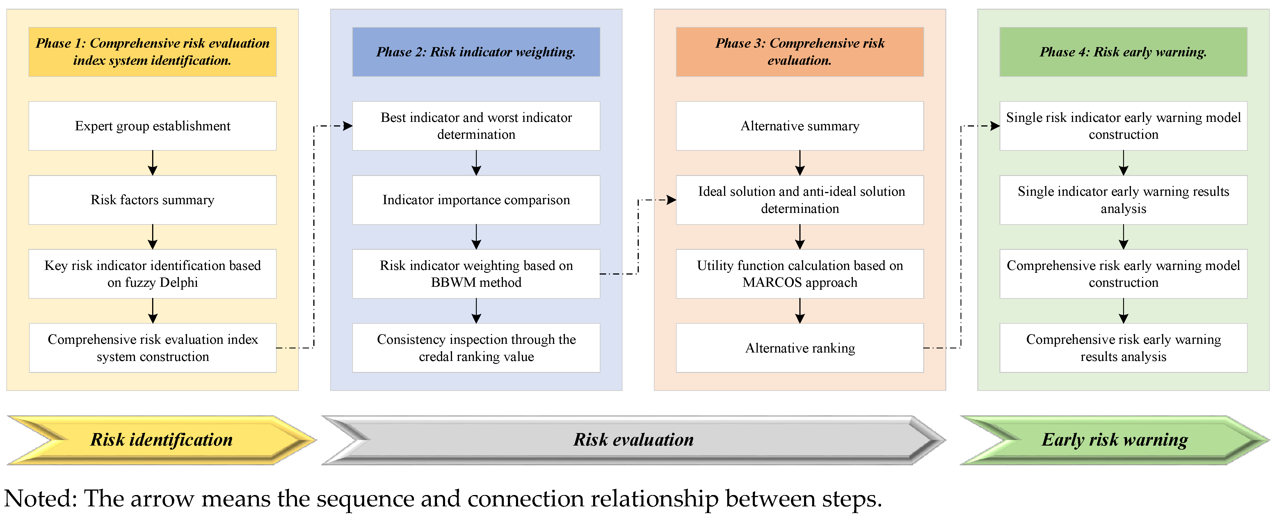
In this paper, a comprehensive risk management framework of HPGE is constructed, as shown in Figure 1.

➢

Phase 1: Comprehensive risk evaluation index system identification.

First, practitioners of power grid engineering and university professors engaged in relevant fields are invited to be members of the expert group. Then, the risk factors affecting high-permeability power grid engineering are summarized. Next, the key risk indicators are identified based on the fuzzy Delphi method. Finally, the comprehensive risk assessment index system is constructed.

➢

Phase 2: Risk indicator weighting.

First, the experts need to determine the best and worst indicators. Then, they should compare the importance of the best and worst indicators with other indicators. Next, the Bayesian BWM method is adopted to determine the weight of each risk indicator. Finally, the consistency of the experts’ opinions is checked by calculating the credal ranking value.

➢

Phase 3: Comprehensive risk evaluation.

First, the alternatives are summarized and the performance of each alternative on each risk indicator is sorted out. Then, both the ideal and anti-ideal solutions are determined. Next, the utility function based on the MARCOS approach is calculated. Finally, all the alternatives are ranked.

➢

Phase 4: Early risk warning.

Based on the previous risk assessment results, the early risk warning of HPGE can be further processed. First, the single risk indicator early warning model is constructed. Then, the single indicator early warning results of each indicator for all the alternatives are analyzed. Next, the comprehensive early risk warning model is constructed. Finally, the comprehensive early warning results for all the alternatives are analyzed.

4. Empirical Analysis

4.1. Data Sources

To verify the effectiveness and superiority of the comprehensive risk management framework put forth in this research, we carried out an empirical analysis in this section. The foundational information for HPGE originates from a southern Chinese province’s prefecture-level city. The province, which is a major center for renewable energy in southern China, has 80 million kilowatts of installed power-producing capacity; among this amount, the installed capacity for clean energy has surpassed 60%. The safe and steady operation of the local power system is also faced with additional issues due to the high percentage of renewable energy.

In light of this, we selected ten scheduled HPGE projects from the region’s project library as examples and established a comprehensive risk management and control mechanism throughout the entire process. Based on the framework presented in Section 3.5, we first compiled a list of all the potential hazards that HPGE could encounter during construction and operation. Then, the most significant risk indicators are identified. Secondly, we calculate the weights of indicators and evaluate the comprehensive risks of ten HPGE projects. Finally, each HPGE’s risk alert status is further estimated. According to the early warning results, we will postpone building for those with high warning levels, and give construction priority to low-risk HPGE projects. The computer used in the empirical analysis had an i7-1185G7 processor, 32 GB memory, and the simulation platform was Matlab 2018b.

4.2. Comprehensive Risk Evaluation Index System Construction

4.2.1. HPGE Risk Factors Analysis

We first invited five experts engaged in relevant fields to form the expert group (including power grid enterprise employees, HPGE designers, and professors). Then, the expert group discussed the risk factors that may affect HPGE through their experience and knowledge. The risk factors are summarized in

Table 4. The risk factors affecting the HPGE summarized by experts.

Target Layer	Risk Dimension	Risk Factor
High-permeability power grid engineering risks	Policy risk (R1)	Construction of new power system (R11)
		Clean energy consumption policy (R12)
		Regulatory policy of transmission and distribution electricity price (R13)
		Environmental protection policy (R14)
	Management risk (R2)	Quality Assurance (R21)
		Contract management (R22)
		Progress management (R23)
		Personnel management (R24)
		Security management (R25)
	Financial risk (R3)	Factor market price fluctuation (R31)
		Transmission-distribution price (R32)
		Financing capacity (R33)
	Operation risk (R4)	Clean energy transmission power (R41)
		Power supply reliability (R42)
		Load rate (R43)
		Voltage qualification rate (R44)
		Number of unplanned outages (R45)
	Technical environmental risk (R5)	Clean energy penetration (R51)
		Electrification rate of terminal energy consumption (R52)
		Flexible and adjustable resource proportion (R53)
	Natural environmental risk (R6)	Natural disaster (R61)
		Geological conditions (R62)
	Social environmental risk (R7)	Compensation for land acquisition and demolition (R71)
		Social public opinion (R72)

.

➢

Policy risk (R1)

When the national macro policy changes or the local policy is adjusted, the construction and operation of the engineering facility may be affected. Therefore, analyzing the policy risks faced by high-permeability power grid engineering is necessary. High-permeability grid engineering is an important means for the construction and development of new power systems, focusing on large-scale access to renewable energy such as wind power and photovoltaics. Hence, the construction of a new power system (R11) and a clean energy consumption policy (R12) are taken into consideration. In addition, the regulatory policy of the transmission and distribution of electricity prices (R13) and the environmental protection policy (R14) are also the key policy risk points faced by the PGPs. It is necessary to judge the compliance of the project according to the policy changes.

➢

Management risk (R2)

Any project will face management risk, including HPGEs. The expert group summarized the five most common management risks in the project, including quality assurance risks (R21), contract management (R22), progress management risks (R23), personnel management (R24), and security management (R25).

➢

Financial risk (R3)

The financial risk of a PGP mainly comes from three aspects. The first is the investment and operation cost of the project, which is affected by the fluctuation of the factor market price (R31). Secondly, the transmission and distribution of electricity prices (R32) is the key factor determining the profitability of the project. Finally, the financing capacity (R33) of the project owner also has a key impact on the smooth implementation of the project.

➢

Operation risk (R4)

The operation risk of the project refers to whether the project can achieve the expected operational objectives. First, clean energy transmission power (R41) is selected to reflect the transmission capacity of the project. Secondly, the quality of the power supply is also a key factor affecting the operation of the project, including power supply reliability (R42), load rate (R43), and voltage qualification rate (R44). Finally, safety and stability are also important aspects that affect the operation of the project; as such, the number of unplanned outages (R45) is selected.

➢

Technical environmental risk (R5)

The construction of high-permeability power grids cannot be separated from the local technical environment. If the clean energy penetration (R51) is high, it is necessary to build a high-permeability power grid to guarantee the safety and steadiness of the power grid. On the contrary, if the proportion of clean energy is low and the demand for high-permeability PGPs is insufficient, the project’s expected benefits may be difficult to achieve. Similarly, if the electricity rate of terminal energy consumption (R52) in the region is low, the demand for the project will also decrease synchronously. Finally, the flexible and adjustable resource proportion (R53) determines whether the project can be successfully planned. If the local adjustable resources are insufficient, it is difficult to support such a large-scale and high proportion of renewable energy deployment.

➢

Natural environmental risk (R6)

The natural environment risk assessment is an indispensable part of engineering construction. For PGPs, common natural environmental risks mainly include natural disasters (R61) and geological conditions (R62).

➢

Social environmental risk (R7)

As well as the natural environmental risk, social environmental risk is also a risk point to be paid attention to during project construction. For PGPs, common social environmental risks mainly include compensation for land acquisition and demolition (R71) and social public opinion (R72).

4.2.2. Key Risk Factors Identification and Index System Construction

After the determination of the risk factors of HPGE, the expert group needs to identify the key risk factors based on the fuzzy Delphi method proposed in Section 3.1. Through Equations (1)–(3), the risk identification results are obtained, as shown in

Table 5. The risk identification results based on the fuzzy Delphi method.

Indicators	Conservative Value		Optimistic Value		Geometric Mean Value		${\mathit{M}}^{\mathit{i}}\mathbf{-}{\mathit{Z}}^{\mathit{i}}$	Consistent Significance Value
	${\mathit{C}}_{\mathit{L}}^{\mathit{i}}$	${\mathit{C}}_{\mathit{U}}^{\mathit{i}}$	${\mathit{O}}_{\mathit{L}}^{\mathit{i}}$	${\mathit{O}}_{\mathit{U}}^{\mathit{i}}$	${\mathit{C}}_{\mathit{M}}^{\mathit{i}}$	${\mathit{O}}_{\mathit{M}}^{\mathit{i}}$		${\mathit{G}}_{\mathit{i}}$
R11	6	8	9	10	7.2	9.6	1.4	8.4 > 5.5
R12	6	7	7	9	6.6	8	1	7.3 > 5.5
R13	4	5	5	7	4.2	5.6	1.4	4.9 < 5.5
R14	3	3	4	5	3	4.4	1.6	3.7 < 5.5
R21	2	4	3	5	3	3.8	0.2	3.4 < 5.5
R22	2	3	3	4	2.6	3.2	0.8	2.9 < 5.5
R23	3	4	4	6	3.6	5	1	4.3 < 5.5
R24	1	2	2	4	1.8	3	1	2.4 < 5.5
R25	3	4	5	7	3.8	6	2	4.9 < 5.5
R31	2	4	4	5	3	4.6	0.4	3.8 < 5.5
R32	5	6	6	8	5.6	7.4	0.6	6.5 > 5.5
R33	1	3	3	4	2	3.4	0.6	2.7 < 5.5
R41	6	7	7	9	6.4	8	1	7.2 > 5.5
R42	4	6	5	7	5.4	5.8	0.2	5.6 > 5.5
R43	5	6	7	8	5.8	7.8	1.2	6.8 > 5.5
R44	3	6	5	7	4.4	6	0	5.4 < 5.5
R45	4	6	6	7	5.4	6.6	0.4	6.0 > 5.5
R51	5	7	8	9	6.4	8.4	1.6	7.4 > 5.5
R52	5	6	6	7	5.8	6.4	0.6	6.1 > 5.5
R53	4	5	6	8	4.2	6.4	2.6	5.3 < 5.5
R61	4	5	4	6	4.4	4.8	0.2	4.6 < 5.5
R62	3	4	4	5	3.4	4.4	0.6	3.9 < 5.5
R71	1	3	3	4	2	3.4	0.6	2.7 < 5.5
R72	2	3	3	4	2.2	3.2	0.8	2.7 < 5.5

.

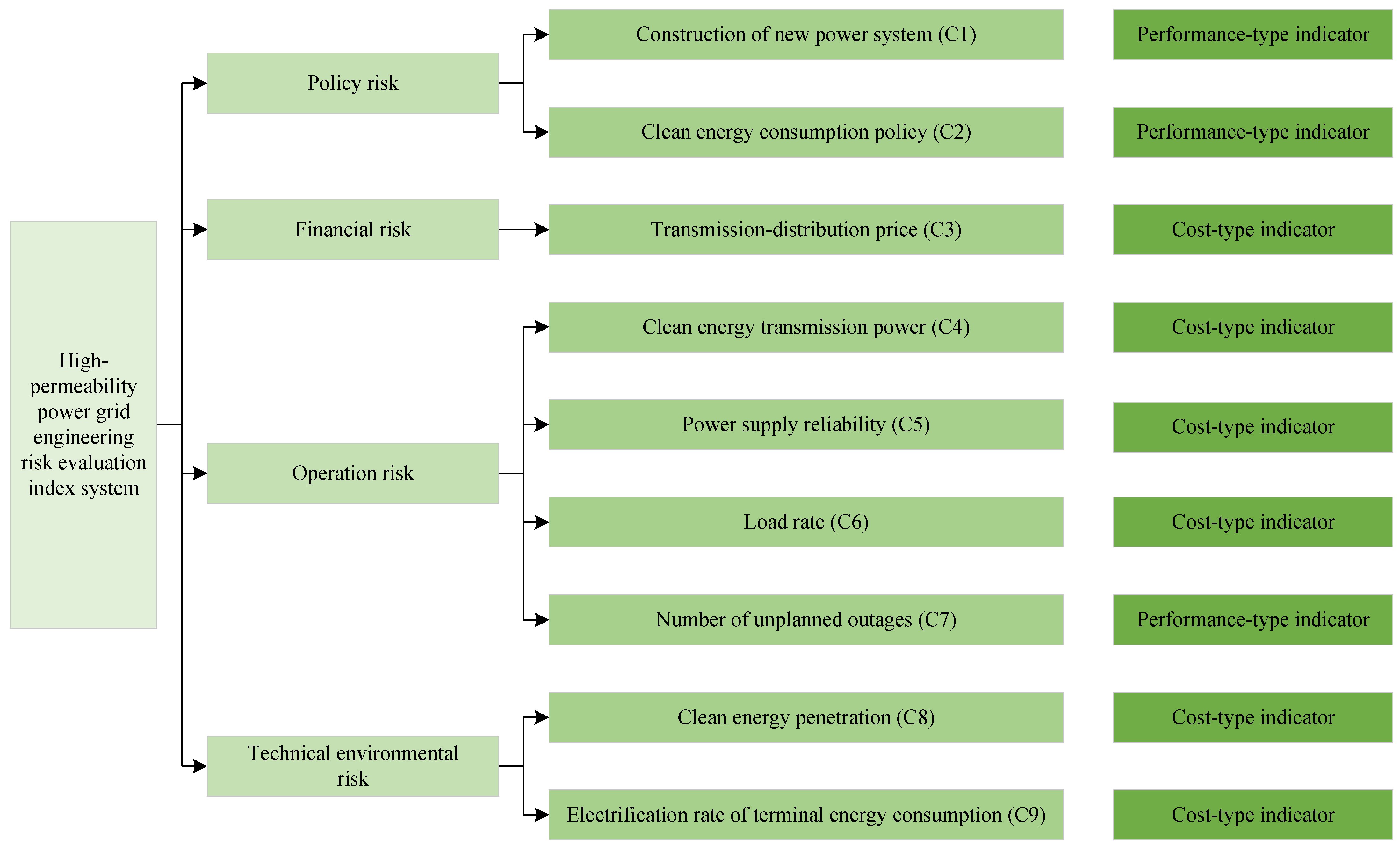
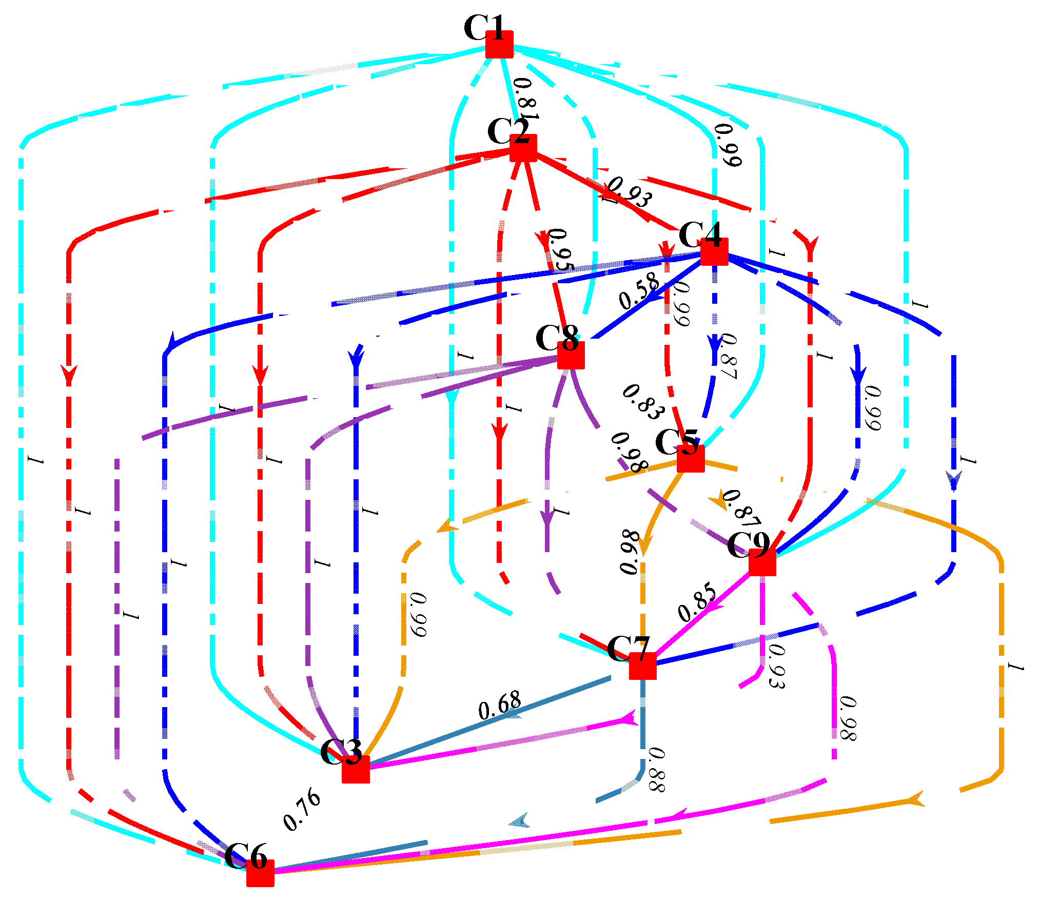
From Table 5, the key risk indicators affecting the HPGE can be further screened out. Then, the risk evaluation index system is composed of these indicators, as shown in Figure 2.

From the seven risk dimensions indicated in Table 4, the expert group places greater emphasis on risks related to policy, finance, operations, and the technological environment. In contrast, the impact of management and risks related to the natural and social environments are not given as much attention. The primary cause of this occurrence is that the expert group pays more attention to risk factors that are highly related to the characteristics of HPGE, and while management risks are common in any engineering facility, they are not the key factors affecting HPGE.

Specifically, the construction of new power systems (C1) and the clean energy consumption policy (C2) are thought to be major risk factors; of these, the former shows that updates and amendments to regulations pertaining to the building of new power systems can readily impact the project’s licensing or performance, while the latter highlights that changing the proportion of renewable energy consumption may affect the construction demand of HPGE. Regarding the financial risk dimension, the transmission–distribution price (C3) has a direct impact on the HPGE’s revenue level, which is also one of the primary financial risk factors. Clean energy transmission power (C4), power supply reliability (C5), load rate (C6), and the number of unscheduled outages (C7) are chosen based on the operating risk dimension. If the clean energy transmission power exceeds expectations, the demand for HPGE from the power grid will increase synchronously. On the contrary, if the power transmission is insufficient, most HPGE projects will be abandoned, resulting in an extremely low efficiency. Similarly, C5, C6, and C7 are the core indicators that reflect the effectiveness of engineering operations, which should likewise be given priority. Regarding the technical environmental risk, clean energy penetration (C8) and the electrification rate of terminal energy consumption (C9) are selected, and the mechanism of action is largely identical to that of C4.

4.3. Risk Indicator Weighting

According to the basic steps of the Bayesian BWM mentioned in Section 3.2, the best and worst indicators are first selected by the experts within the expert group, as listed in

Table 6. The best and worst indicators selected by the experts within the expert group.

Expert Number	Best Indicator	Worst Indicator
1	C1	C6
2	C1	C3
3	C1	C6
4	C1	C6
5	C1	C6

.

Then, the optimal and worst comparison vectors $A_B^{1:K}$ and $A_W^{1:K}$ are shown as follows:

$${\mathit{A}}_{\mathrm{B}}^{1:5}=\left(\begin{array}{rrrrrrrrr}\hfill 1& \hfill 2& \hfill 8& \hfill 3& \hfill 5& \hfill 9& \hfill 7& \hfill 4& \hfill 6\\ \hfill 1& \hfill 2& \hfill 9& \hfill 3& \hfill 5& \hfill 8& \hfill 7& \hfill 4& \hfill 6\\ \hfill 1& \hfill 2& \hfill 7& \hfill 4& \hfill 6& \hfill 9& \hfill 8& \hfill 3& \hfill 5\\ \hfill 1& \hfill 2& \hfill 7& \hfill 4& \hfill 3& \hfill 9& \hfill 8& \hfill 5& \hfill 6\\ \hfill 1& \hfill 2& \hfill 8& \hfill 4& \hfill 5& \hfill 9& \hfill 6& \hfill 3& \hfill 7\end{array}\right){\mathit{A}}_{\mathrm{W}}^{1:5}=\left(\begin{array}{rrrrrrrrr}\hfill 9& \hfill 8& \hfill 2& \hfill 7& \hfill 5& \hfill 1& \hfill 3& \hfill 6& \hfill 4\\ \hfill 9& \hfill 8& \hfill 1& \hfill 7& \hfill 5& \hfill 2& \hfill 3& \hfill 6& \hfill 4\\ \hfill 9& \hfill 8& \hfill 3& \hfill 6& \hfill 4& \hfill 1& \hfill 2& \hfill 7& \hfill 5\\ \hfill 9& \hfill 8& \hfill 3& \hfill 6& \hfill 7& \hfill 1& \hfill 2& \hfill 5& \hfill 4\\ \hfill 9& \hfill 8& \hfill 2& \hfill 6& \hfill 5& \hfill 1& \hfill 4& \hfill 7& \hfill 3\end{array}\right)$$

Next, the weights of risk indicators for HPGEs are calculated based on the Bayesian BWM; these are listed in

Table 7. The weights of risk indicators for HPGE.

Indicator	Weight	Indicator	Weight
C1	0.2176	C6	0.0458
C2	0.1823	C7	0.0612
C3	0.0546	C8	0.1262
C4	0.1324	C9	0.0782
C5	0.1017

.

As shown in Table 7, the introduction and adjustment of relevant policies will directly affect the construction and operation of power grid engineering. Thus, the weights of the construction of new power systems (C1) and the clean energy consumption policy (C2) are the highest of all nine indicators. Of these indicators, the policies related to the construction and development of new power systems will bring the greatest risk to the PGPs. In contrast, the weights of load rate (C6) and transmission–distribution price (C3) are relatively lower, at 0.0458 and 0.0546, respectively. Generally, the load rate of a PGP is normal in the range of 5% to 80%. If the load rate is low, the incremental benefits may be insufficient, while if the load rate is high, an overload phenomenon will occur, which will affect the safety and reliability of the power system’s operation. However, according to the existing distribution network investment report of State Grid, the load rate of most projects is within the normal range; therefore, the weight value of load risk is small. In addition, although the transmission–distribution price will directly affect the income level of the project, it is a common risk factor in various PGPs. This paper focuses on the risk analysis of high-permeability PGPs and pays more attention to the risk factors that are unique to this type of project. Therefore, the adjustment of the transmission–distribution electricity price brings about only low risks to the project.

To ensure the rationality of index weight assignment, it is necessary to carry out consistency tests through credal ranking. The credal ranking results of the risk indicators for HPGE are shown in Figure A1; it can be seen that all the credal ranking values are greater than 0.5 (the threshold of decision consistency), which indicates that all experts have consistency in the weighting results of indicators. Different from the traditional ranking schemes, credal ranking is computed in the Dirichlet distribution. In 2019, Mohammadi and Rezaei proved why 0.5 is the consistency discrimination criteria through mathematical formulas; interested readers can refer to Ref. [36].

4.4. Comprehensive Risk Evaluation

After determining the weights of the risk indicators, we can assess the comprehensive risk of each HPGE. In this paper, ten HPGEs (EI~E10) are selected for comprehensive risk assessment. Since the constructed indicator system includes both qualitative and quantitative indicators, the actual values are used in the evaluation of quantitative indicators, and a score of 1–10 points is used in the evaluation of qualitative indicators, whereby the higher the score, the greater the risk.

According to the MARCOS approach, we first established the initial decision-making matrix, which is listed as follows:

As shown in

Table 8. The initial decision-making matrix.

	C1	C2	C3	C4	C5	C6	C7	C8	C9
E1	3	2	0.0658	85.3	99.92%	66.50%	2	41.20%	10.40%
E2	3	2	0.1092	56.7	99.88%	44.50%	1	28.20%	7.04%
E3	3	2	0.0608	117.5	99.92%	76.20%	3	65.90%	18.91%
E4	2	4	0.16	19.5	99.93%	22.70%	1	14.70%	12.00%
E5	1	3	0.0668	175	99.82%	78.50%	2	20.95%	12.68%
E6	3	3	0.1235	80.5	99.81%	53.80%	1	7.00%	10.70%
E7	4	3	0.0559	68.2	99.84%	55.50%	3	60.70%	46.48%
E8	3	3	0.1579	34.1	99.95%	31.80%	2	18.70%	29.60%
E9	2	3	0.1153	61.4	99.92%	47.20%	1	16.29%	17.48%
E10	3	3	0.0885	40.3	99.95%	46.80%	2	18.97%	8.90%

, different engineering facilities have different performances for each indicator. It is worth mentioning that the heterogeneity between various projects is not very obvious in the index of power supply reliability (C5). If it is directly normalized, each project may have almost the same performance results on this indicator. Therefore, we have dealt with this indicator by reducing the power supply reliability of each project by 99.8% (99.8% is the basic value of power supply reliability required in the “Ten Commitments” of the power supply service of SGGC). Then, the normalization matrix can be obtained using Equations (12) and (13), as depicted in

Table A1. The normalization decision-making matrix.

	C1	C2	C3	C4	C5	C6	C7	C8	C9
E1	0.7500	0.5000	0.8495	0.2286	0.0948	0.3414	0.6667	0.1699	0.6772
E2	0.7500	0.5000	0.5119	0.3439	0.1429	0.5101	0.3333	0.2482	1.0000
E3	0.7500	0.5000	0.9194	0.1660	0.0887	0.2979	1.0000	0.1062	0.3724
E4	0.5000	1.0000	0.3494	1.0000	0.0833	1.0000	0.3333	0.4762	0.5867
E5	0.2500	0.7500	0.8368	0.1114	0.4783	0.2892	0.6667	0.3341	0.5555
E6	0.7500	0.7500	0.4526	0.2422	1.0000	0.4219	0.3333	1.0000	0.6582
E7	1.0000	0.7500	1.0000	0.2859	0.2973	0.4090	1.0000	0.1153	0.1515
E8	0.7500	0.7500	0.3540	0.5718	0.0733	0.7138	0.6667	0.3743	0.2379
E9	0.5000	0.7500	0.4848	0.3176	0.0948	0.4809	0.3333	0.4298	0.4029
E10	0.7500	0.7500	0.6316	0.4839	0.0733	0.4850	0.6667	0.3690	0.7910

. According to the weights of the indicators calculated in Table 7, the weighted normalization matrix can be obtained, as depicted in

Table A2. The weighted normalization decision-making matrix.

	C1	C2	C3	C4	C5	C6	C7	C8	C9
E1	0.1632	0.0912	0.0464	0.0303	0.0096	0.0156	0.0408	0.0214	0.0530
E2	0.1632	0.0912	0.0280	0.0455	0.0145	0.0234	0.0204	0.0313	0.0782
E3	0.1632	0.0912	0.0502	0.0220	0.0090	0.0136	0.0612	0.0134	0.0291
E4	0.1088	0.1823	0.0191	0.1324	0.0085	0.0458	0.0204	0.0601	0.0459
E5	0.0544	0.1367	0.0457	0.0148	0.0486	0.0132	0.0408	0.0422	0.0434
E6	0.1632	0.1367	0.0247	0.0321	0.1017	0.0193	0.0204	0.1262	0.0515
E7	0.2176	0.1367	0.0546	0.0379	0.0302	0.0187	0.0612	0.0146	0.0118
E8	0.1632	0.1367	0.0193	0.0757	0.0075	0.0327	0.0408	0.0472	0.0186
E9	0.1088	0.1367	0.0265	0.0420	0.0096	0.0220	0.0204	0.0542	0.0315
E10	0.1632	0.1367	0.0345	0.0641	0.0075	0.0222	0.0408	0.0466	0.0619

.

Then, the ideal and anti-ideal solutions can be obtained, as depicted in

Table 9. The ideal and anti-ideal solution.

	C1	C2	C3	C4	C5	C6	C7	C8	C9
$S^{+}$	0.2176	0.1823	0.0546	0.1324	0.1017	0.0458	0.0612	0.1262	0.0782
$S^{-}$	0.0544	0.0912	0.0191	0.0148	0.0075	0.0132	0.0204	0.0134	0.0118

. Furthermore, the utility degree of each HPGE is calculated and is shown in

Table 10. The utility degree of each HPGE.

	E1	E2	E3	E4	E5	E6	E7	E8	E9	E10
$K{(j)}^{+}$	4.2781	4.3403	4.2006	5.3290	4.2720	5.6083	5.0091	4.4920	3.7942	5.0006
$K{(j)}^{-}$	19.0255	22.2002	16.8183	27.9241	22.2284	37.8231	21.4824	21.2082	18.3992	24.0222

.

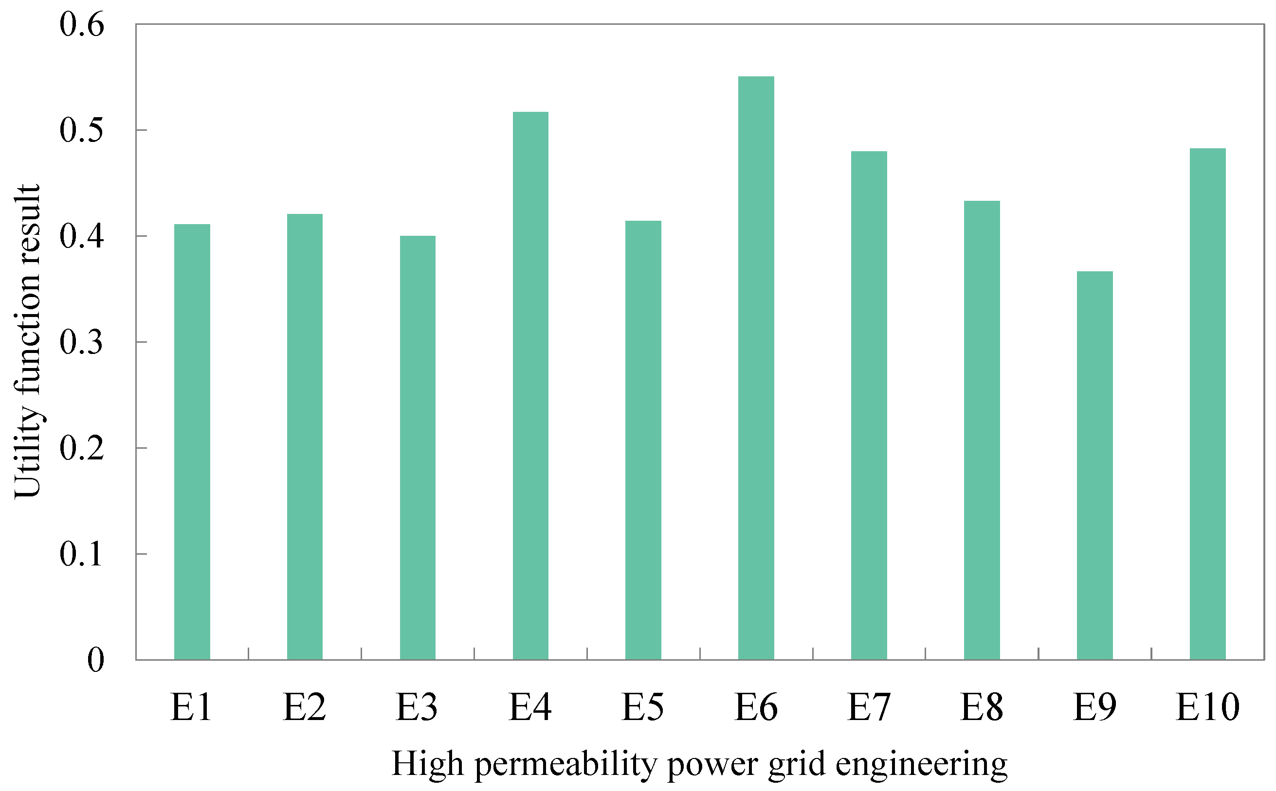
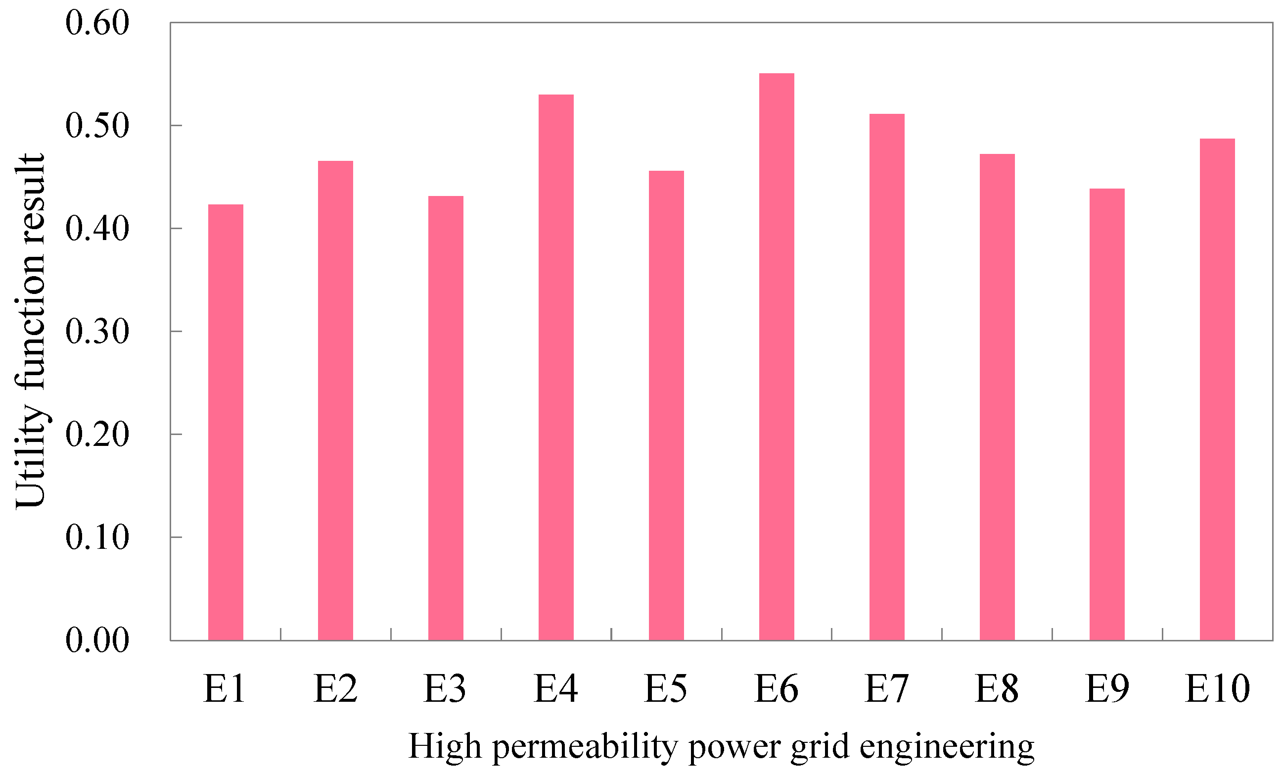
Finally, the utility function of each engineering facility is obtained using Equation (17); the risk evaluation results are shown in Figure 3.

As shown in Figure 3, the risk ranking of the ten HPGEs is E6 > E4 > E10 > E7 > E8 > E2 > E5 > E1 > E3 > E9. Although E6 has a relatively good performance in relation to the C3, C4, and C7 indicators, it has the best performance in the E7 indicators of all ten projects. However, it also has a poor performance in the C1, C2, and C8 indicators with higher weights, resulting in a higher overall risk for the engineering facility. In contrast, E9 has a low risk in the most important indicators; therefore, the comprehensive risk of E9 is the lowest.

4.5. Early Risk Warning Results

4.5.1. Early Risk Warning for a Single Indicator

First, the risk value of each indicator for all the alternatives is given in

Table 11. The risk value of each indicator for all the alternatives.

	C1	C2	C3	C4	C5	C6	C7	C8	C9
E1	30	20	84	57	42	18	40	59	79
E2	30	20	41	72	61	47	20	65	86
E3	30	20	89	41	38	5	60	18	62
E4	20	40	0	90	34	76	20	82	76
E5	10	30	83	13	89	2	40	74	75
E6	30	30	27	60	94	35	20	91	79
E7	40	30	94	66	82	33	60	24	7
E8	30	30	0	83	25	64	40	77	41
E9	20	30	35	69	42	44	20	80	65
E10	30	30	62	80	25	44	40	76	82

.

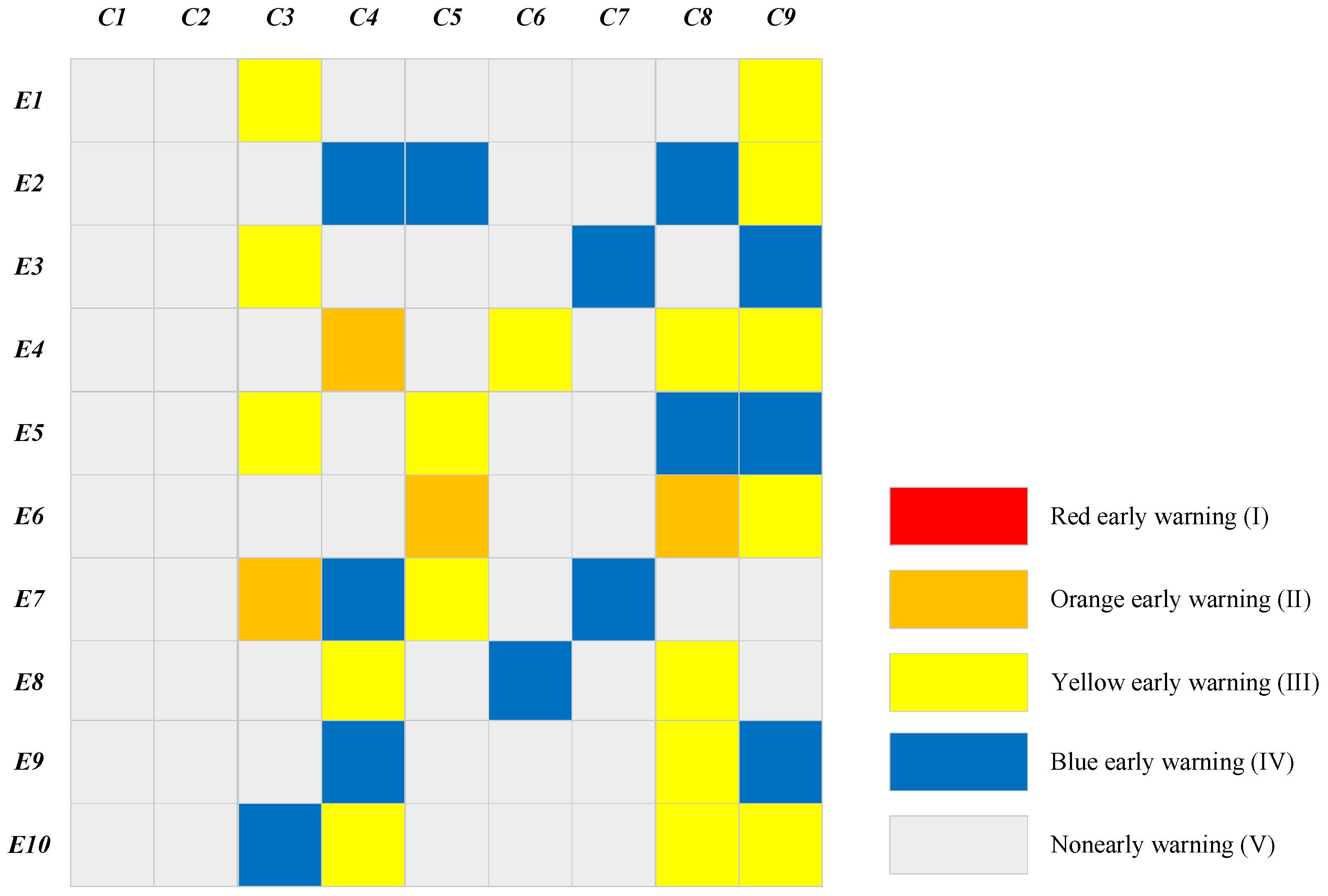
According to Equation (18), the early warning value and level of a single indicator for all the alternatives are calculated, as shown in Figure 4.

As shown in Figure 4, the early warning results of every single indicator also confirm the results of the project risk assessment. Specifically, E4 engineering has one indicator (C4) in the level II early warning state and three indicators (C6, C8, and C9) in the level III early warning state. In contrast, E9 engineering has one indicator (C8) in the level III early warning state, and two indicators (C4 and C9) in the level IV early warning state. From the perspective of indicator dimension, the C8 and C9 indicators have the most serious early warning situations. Specifically, seven projects are in the level II to level IV early warning state on C8 indicators, and eight projects are in the level III to level IV early warning state on C9 indicators.

4.5.2. Early Risk Warning for the Entire HPGE

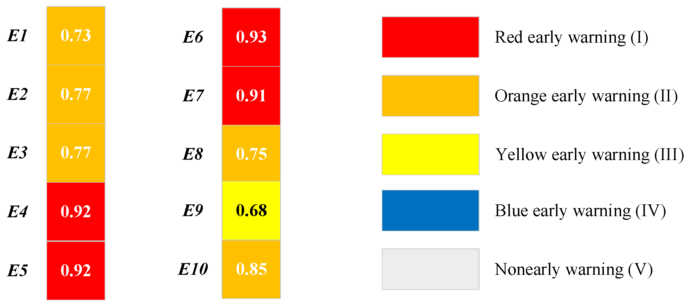
Then, the comprehensive early risk warning value of all the alternatives can be obtained, as shown in Figure 5.

As shown in Figure 5, there are four projects in the level I early risk warning state, five projects in the level II early risk warning state, and one project in the level III early risk warning state.

4.6. Evaluation Results Comparison

In order to prove the effectiveness and superiority of the proposed Bayesian BWM–MARCOS approach in risk evaluation, we established two comparison scenarios, as follows:

4.6.1. Comparison from the Dimension of Indicator Weighting

Compared with the traditional BWM, the Bayesian BWM adopted can introduce the group decision-making process and enhance the rationality of weighting. The weight of each risk indicator for HPGE obtained using the BWM is listed in

Table 12. The weight of each risk indicator for HPGE obtained by BWM.

Expert	Weight
	C1	C2	C3	C4	C5	C6	C7	C8	C9
1	0.3146	0.1915	0.0479	0.1277	0.0766	0.0274	0.0547	0.0958	0.0638
2	0.3146	0.1915	0.0274	0.1277	0.0766	0.0479	0.0547	0.0958	0.0638
3	0.3146	0.1915	0.0547	0.0958	0.0638	0.0274	0.0479	0.1277	0.0766
4	0.3146	0.1915	0.0547	0.0958	0.1277	0.0274	0.0479	0.0766	0.0638
5	0.3146	0.1915	0.0479	0.0958	0.0766	0.0274	0.0638	0.1277	0.0547
Average	0.3146	0.1915	0.0465	0.1086	0.0843	0.0315	0.0538	0.1047	0.0645

.

As shown in Table 12, the Bayesian BWM used in this paper is consistent with the weight ranking of each index obtained using the BWM, and the ranking of the indicators is as follows: C1 > C2 > C4 > C8 > C5 > C9 > C7 > C3 > C6. The difference is that the BWM is easy to expand the heterogeneity between indicators. The weight of the best indicator calculated using the BWM is 0.3146, which is nearly ten times that of the worst indicator (0.0315). On the contrary, through the Bayesian BWM, the weight of the most important indicator is only five times that of the worst indicator. The excessive heterogeneity of indicator weights may easily lead to the neglect and the amplification of the role of some indicators, thus affecting the final risk assessment results.

4.6.2. Comparison from the Dimension of Comprehensive Evaluation

Compared with the traditional TOPSIS method, the proposed MARCOS approach simultaneously considers the influence of the ideal and anti-ideal solutions on the comprehensive evaluation results. The risk evaluation result of each engineering facility based on the TOPSIS method is shown in Figure 6.

As shown in Figure 5, the risk ranking of the ten HPGE based on the TOPSIS method is E6 > E4 > E7 > E10 > E2 > E8 > E5 > E9 > E3 > E1. To prove the MARCOS approach has better ranking performance, four indices are applied to measure the ranking effect of each method: standard deviation $\sigma$, relative range $\theta$, coefficient of variation $\nu$, and sensitivity $\eta$.

$$\{\begin{array}{l}\sigma =\sqrt{\frac{{\displaystyle {\sum }_{j=1}^m{({\delta }_j-\stackrel{-}{\delta })}^2}}{m}}\\ \theta =\frac{{\delta }_{j,max}-{\delta }_{j,min}}{\stackrel{-}{\delta }}\times 100\%\\ \nu =\sigma /\stackrel{-}{\delta }\\ \eta =\frac{{\delta }_{j,max}-{\delta }_{j,sec}}{{\delta }_{j,max}}\end{array}$$

(20)

where ${\delta }_j$ represents the relative proximity of each alternative to the ideal solution, $\stackrel{-}{\delta }$ represents the mean value of ${\delta }_j$, ${\delta }_{j,max}$ and ${\delta }_{j,min}$ represent the maximum and minimum values of ${\delta }_j$, and ${\delta }_{j,sec}$ represents the second largest value of ${\delta }_j$. The above four indicators are all performance-type indices. In other words, the larger the indicator value, the better the sample separation effects of the model.

The sample separation for the TOPSIS method and the MARCOS approach are listed in

Table 13. The sample separation index for the TOPSIS method and the MARCOS approach.

Model	Sample Separation Effect Index
	$\mathit{\sigma }$	$\mathit{\theta }$	$\mathit{\nu }$	$\mathit{\eta }$
TOPSIS	0.0544	39.16%	0.1175	0.0498
MARCOS	0.0659	75.00%	0.2233	0.0550

.

As shown in Table 13, the sample separation performance of the MARCOS approach is better than that of the TOPSIS method.

5. Conclusions and Limitations

5.1. Conclusions

The proposal of the “dual carbon” climate goals and the construction of new power systems have brought about new challenges to HPGE, which not only require the strengthening of the security and stability of power grid transmission, but also steadily increase the access proportion of clean energy. In this context, a three-stage comprehensive risk management framework for HPGE is constructed in this paper, and several conclusions can be obtained as follows:

(1) At present, HPGEs are facing seven major risks from internal and external sources. Of these risks, those concerning policy, finance, operation, and the technical environment are identified to be the most important risk factors based on the fuzzy Delphi method. In the HPGE comprehensive risk assessment index system that includes nine key risk indicators, new power system construction-related and clean energy consumption-related policies are considered to be the most important factors affecting HPGE construction and operation. Therefore, in the follow-up HPGE project planning and construction, it is necessary to pay attention to the latest developments of relevant policies.

(2) Although policy factors have the highest risk, most HPGE projects, in fact, strictly comply with relevant laws, regulations, and policy trends. In contrast, HPGE projects face greater risks in terms of the clean energy penetration rate and the electrification rate of terminal energy consumption. Most HPGE projects have medium-to-high risk warning levels in these two aspects. In the context of the current energy transformation and energy structure adjustment, the large-scale construction, development, and utilization of clean energy have become the general trend. Therefore, in the process of subsequent HPGE project construction, it is necessary to strengthen risk prevention and develop a closed-loop management and control mechanism containing risk identification, risk evaluation, and early risk warning.

(3) From the perspective of risk research methods, the adopted Bayesian BWM has a better weighting performance compared with the traditional BWM, which can reduce the heterogeneity between indicator weights. Compared with TOPSIS, the MARCOS approach has a better sample separation performance. In addition, the traditional early risk warning model ignores the non-compensation between indicators. Even if there is a serious early warning phenomenon in one indicator, it is still possible to lower the early warning level through the better performance of other indicators. The early warning model based on the multiplicative synthesis technique proposed in this paper is much closer to the realistic situation of engineering operations.

5.2. Future Directions and Limitations

Through the proposed HPGE’s entire-process risk management technology, we may offer guidance for investment decisions for power grid companies in the region. Furthermore, other PGP applications can make further use of the models employed in this work. It is important to acknowledge that the focus of this work is HPGE, which presents distinct risks in contrast to conventional power grid engineering. Therefore, when applying the methods to conduct risk assessments on other types of PGPs, it is necessary to separately analyze and sort out risk indicators for different types of projects.

In addition, due to sample size limitations, we only conducted risk analysis on ten HPGEs. In future research, we will further expand our research scope and conduct risk analysis and treatment for HPGEs in different regions and with different characteristics.

References

1. Zhao, Y.; Su, Q.; Li, B.; Zhang, Y.; Wang, X.; Zhao, H.; Guo, S. Have those countries declaring “zero carbon” or “carbon neutral” climate goals achieved carbon emissions-economic growth decoupling? J. Clean. Prod. 2022, 363, 132450. [Google Scholar] [CrossRef]
2. Zheng, J.; Mi, Z.; Coffman, D.; Milcheva, S.; Shan, Y.; Guan, D.; Wang, S. Regional development and carbon emissions in China. Energy Econ. 2019, 81, 25–36. [Google Scholar] [CrossRef]
3. Wang, X.; Fan, F.; Liu, C.; Han, Y.; Liu, Q.; Wang, A. Regional differences and driving factors analysis of carbon emissions from power sector in China. Ecol. Indic. 2022, 142, 109297. [Google Scholar] [CrossRef]
4. Yang, Z.; Yang, F.; Min, H.; Tian, H.; Hu, W.; Liu, J. Review on optimal planning of new power systems with distributed generations and electric vehicles. Energy Rep. 2023, 9, 501–509. [Google Scholar] [CrossRef]
5. Li, H.; Sun, D.; Li, B.; Wang, X.; Zhao, Y.; Wei, M.; Dang, X. Collaborative optimization of VRB-PS hybrid energy storage system for large-scale wind power grid integration. Energy 2023, 265, 126292. [Google Scholar] [CrossRef]
6. Wang, J. Construction of Risk Evaluation Index System for Power Grid Engineering Cost by Applying WBS-RBS and Membership Degree Methods. Math. Probl. Eng. 2020, 2020, 6217872. [Google Scholar] [CrossRef]
7. Jiang, Q.; Huang, R.; Huang, Y.; Chen, S.; He, Y.; Lan, L.; Liu, C. Application of BP Neural Network Based on Genetic Algorithm Optimization in Evaluation of Power Grid Investment Risk. IEEE Access 2019, 7, 154827–154835. [Google Scholar] [CrossRef]
8. Li, C.; Liu, Y.; Li, S. Risk Evaluation of Qinghai–Tibet Power Grid Interconnection Project for Sustainability. Sustainability 2016, 8, 85. [Google Scholar] [CrossRef]
9. You, L.; Ma, H.; Saha, T. A CVaR-constrained optimal power flow model for wind integrated power systems considering Transmission-side flexibility. Int. J. Electr. Power Energy Syst. 2023, 150, 109087. [Google Scholar] [CrossRef]
10. Yang, L.; Chen, Y.; Qiu, Q.; Wang, J. Risk Control of Mission-Critical Systems: Abort Decision-Makings Integrating Health and Age Conditions. IEEE Trans. Ind. Inform. 2022, 18, 6887–6894. [Google Scholar] [CrossRef]
11. Yang, L.; Wei, F.; Qiu, Q. Mission risk control via joint optimization of sampling and abort decisions. Risk Anal. 2023, 44, 666–685. [Google Scholar] [CrossRef] [PubMed]
12. Fan, W.; Tan, Z.; Li, F.; Zhang, A.; Ju, L.; Wang, Y.; De, G. A two-stage optimal scheduling model of integrated energy system based on CVaR theory implementing integrated demand response. Energy 2023, 263, 125783. [Google Scholar] [CrossRef]
13. Duan, Y.; Sun, Y.; Zhang, Y.; Fan, X.; Dong, Q.; Guo, S. Risk Evaluation of Electric Power Grid Investment in China Employing a Hybrid Novel MCDM Method. Mathematics 2021, 9, 473. [Google Scholar] [CrossRef]
14. Zhou, L.; Cai, L.; Jiang, L.; Chen, L. Power Grid Enterprise Intelligent Risk Identification Model Considering Multi-Attribute and Low Correlation Data. IEEE Access 2019, 7, 111324–111331. [Google Scholar] [CrossRef]
15. Rao, R.; Zhang, X.; Shi, Z.; Luo, K.; Tan, Z.; Feng, Y. A Systematical Framework of Schedule Risk Management for Power Grid Engineering Projects’ Sustainable Development. Sustainability 2014, 6, 6872–6901. [Google Scholar] [CrossRef]
16. Zhang, T.; Yu, W.; Lu, Y.; Chen, L. Identification and Correlation Analysis of Engineering Environmental Risk Factors along the Qinghai–Tibet Engineering Corridor. Remote Sens. 2022, 14, 908. [Google Scholar] [CrossRef]
17. Wang, P.; Wei, Q.; Zhao, G.; Wang, J.; Yin, Y. Safety Risk Identification Method for Railway Construction in Complex and Dangerous Areas. Sustainability 2022, 14, 13698. [Google Scholar] [CrossRef]
18. Zhang, K.; Wang, L.; Liu, J.; Wu, H.; Xu, X.; Huang, D.; Jin, K.; Liu, J. Resilience Capacity Evaluation for the Safety Management System of Power Grid Enterprise Based on AHP-MEE Model. Math. Probl. Eng. 2022, 2022, 8065814. [Google Scholar] [CrossRef]
19. Guo, J.; Xiang, P.; Lee, Y. Analyzing and Controlling Construction Engineering Project Gray Rhino Risks with Innovative MCDM Methods: Interference Fuzzy Analytical Network Process and Decision-Making Trial and Evaluation Laboratory. Appl. Sci. 2022, 12, 5693. [Google Scholar] [CrossRef]
20. Golcuk, I. An interval type-2 fuzzy reasoning model for digital transformation project risk assessment. Expert Syst. Appl. 2020, 159, 113579. [Google Scholar] [CrossRef]
21. Zhang, L.; Wu, J.; Zhang, J.; Su, F.; Bian, H.; Li, L. A dynamic and integrated approach of safety investment decision-making for power grid enterprises. Process Saf. Environ. Prot. 2022, 162, 301–312. [Google Scholar] [CrossRef]
22. Shan, Z.; Long, J.; Yu, P.; Shao, L.; Liao, Y. Lightweight optimization of passenger car seat frame based on grey relational analysis and optimized coefficient of variation. Struct. Multidiscip. Optim. 2020, 62, 3429–3455. [Google Scholar] [CrossRef]
23. Wu, H.; Liu, S.; Wang, J.; Yang, T. Construction Safety Risk Assessment of Bridges in the Marine Environment Based on CRITIC and TOPSIS Models. J. Coast. Res. 2020, 108, 206–210. [Google Scholar] [CrossRef]
24. Koulinas, G.; Demesouka, O.; Marhavilas, P.; Vavatsikos, A.; Koulouriotis, D. Risk Assessment Using Fuzzy TOPSIS and PRAT for Sustainable Engineering Projects. Sustainability 2019, 11, 615. [Google Scholar] [CrossRef]
25. Koc, K.; Gurgun, A. Assessment of Readability Risks in Contracts Causing Conflicts in Construction Projects. J. Constr. Eng. Manag. 2021, 147, 04021041. [Google Scholar] [CrossRef]
26. Mi, J.; Huang, W.; Chen, M.; Zhang, W. A Method of Entropy Weight Quantitative Risk Assessment for the Safety and Security Integration of a Typical Industrial Control System. IEEE Access 2021, 9, 90919–90932. [Google Scholar] [CrossRef]
27. Wang, W.; Lyu, S.; Zhang, Y.; Ma, S. A Risk Assessment Model of Coalbed Methane Development Based on the Matter-Element Extension Method. Energies 2019, 12, 3931. [Google Scholar] [CrossRef]
28. Deng, J. Research on the Risk Early Warning of Construction Engineering under the Coupling Disaster of Typhoons and Rainstorms in Coastal Areas Based on BP Neural Network. J. Coast. Res. 2020, 105, 151–154. [Google Scholar] [CrossRef]
29. He, B.; Bai, M.; Shi, H.; Li, X.; Qi, Y.; Li, Y. Risk Assessment of Pipeline Engineering Geological Disaster Based on GIS and WOE-GA-BP Models. Appl. Sci. 2021, 11, 9919. [Google Scholar] [CrossRef]
30. Wang, X.; Zhang, C.; Deng, J.; Su, C.; Gao, Z. Analysis of Factors Influencing Miners’ Unsafe Behaviors in Intelligent Mines using a Novel Hybrid MCDM Model. Int. J. Environ. Res. Public Health 2022, 19, 7368. [Google Scholar] [CrossRef]
31. Dalkey, N.; Helmer, O. An experimental application of the Delphi method to the use of experts. Manag. Sci. 1963, 9, 458–467. [Google Scholar] [CrossRef]
32. Ishikawa, A.; Amagasa, M.; Shiga, T.; Tomizawa, G.; Tatsuta, R.; Mieno, H. The max-min Delphi method and fuzzy Delphi method via fuzzy integration. Fuzzy Sets Syst. 1993, 55, 241–253. [Google Scholar] [CrossRef]
33. Zhao, H.; Guo, S.; Zhao, H. Comprehensive assessment for battery energy storage systems based on fuzzy-MCDM considering risk preferences. Energy 2019, 168, 450–461. [Google Scholar] [CrossRef]
34. Liang, M.; Li, W.; Ji, J.; Zhou, Z.; Zhao, Y.; Zhao, H.; Guo, S. Evaluating the Comprehensive Performance of 5G Base Station: A Hybrid MCDM Model Based on Bayesian Best-Worst Method and DQ-GRA Technique. Math. Probl. Eng. 2022, 2022, 4038369. [Google Scholar] [CrossRef]
35. Zhang, Y.; Zhao, H.; Li, B.; Zhao, Y.; Qi, Z. Research on credit rating and risk measurement of electricity retailers based on Bayesian Best Worst Method-Cloud Model and improved Credit Metrics model in China’s power market. Energy 2022, 252, 124088. [Google Scholar] [CrossRef]
36. Mohammadi, M.; Rezaei, J. Bayesian best-worst method: A probabilistic group decision making model. Omega 2019, 96, 102075. [Google Scholar] [CrossRef]
37. Rezaei, J. Best-worst multi-criteria decision-making method. Omega 2015, 53, 49–57. [Google Scholar] [CrossRef]
38. Zhang, Z.; Lin, S.; Ye, Y.; Xu, Z.; Zhao, Y.; Zhao, H.; Sun, J. A Hybrid MCDM Model for Evaluating the Market-Oriented Business Regulatory Risk of Power Grid Enterprises Based on the Bayesian Best-Worst Method and MARCOS Approach. Energies 2022, 15, 2978. [Google Scholar] [CrossRef]
39. Zolfani, S.; Bazrafshan, R.; Ecer, F.; Karamasa, C. The Suitability-Feasibility-Acceptability Strategy Integrated with Bayesian BWM-MARCOS Methods to Determine the Optimal Lithium Battery Plant Located in South America. Mathematics 2022, 10, 2401. [Google Scholar] [CrossRef]
40. Li, H.; Li, B.; Yang, G.; Chen, C.; Chen, Y.; Zhao, C. Evaluating the Regulatory Environment of Overseas Electric Power Market Based on a Hybrid Evaluation Model. Int. J. Fuzzy Syst. 2020, 22, 138–155. [Google Scholar] [CrossRef]
Figure 1. Comprehensive risk management framework of HPGE.
Energies 17 03439 g001
Figure 2. The comprehensive risk assessment index system of HPGE.
Energies 17 03439 g002
Figure 3. The utility function results of HPGE.
Energies 17 03439 g003
Figure 4. The early warning value and level of a single indicator for all the alternatives.
Energies 17 03439 g004
Figure 5. The comprehensive early risk warning value of all the alternatives.
Energies 17 03439 g005
Figure 6. The risk evaluation result of each engineering system based on the TOPSIS method.
Energies 17 03439 g006