Article

Analysis of the Measurement of Transportation Carbon Emissions and the Emission Reduction Path in the Yangtze River Economic Belt under the Background of “Dual Carbon” Goals

1
School of Transportation, Shandong University of Science and Technology, Qingdao 266590, China
2
International Cooperation Center of National Development and Reform Commission, Beijing 100038, China
*
Author to whom correspondence should be addressed.
Energies 2024, 17(14), 3364; https://doi.org/10.3390/en17143364
Submission received: 1 June 2024 / Revised: 24 June 2024 / Accepted: 4 July 2024 / Published: 9 July 2024
(This article belongs to the Section B: Energy and Environment)

Abstract

:
Carbon emissions from the Yangtze River Economic Belt are an important element of China’s carbon emission endeavor, and a study of its emission reduction pathway can provide a reference for the country’s overall management of carbon emission reduction. From the perspective of energy consumption, this paper uses the carbon emission factor method to estimate the carbon emissions of the transportation industry in the Yangtze River Economic Belt during 2006–2020, based on the extended STIRPAT model, considering the influence of seven factors, i.e., population size, urbanization rate, GDP per capita, transportation added value, energy structure, energy intensity, and transportation intensity, on carbon emissions. Based on these factors, a scenario analysis, combined with a forecasting model, is used to predict the peak carbon performance of the transportation industry under different development scenarios. The results show that the overall carbon emissions of transportation in the YEB from 2006 to 2020 show a fluctuating upward trend, and the downstream carbon emissions are significantly higher than those in other regions. The main factors influencing carbon emissions from transportation in different upstream, midstream, and downstream regions vary, with both population and economic factors contributing to carbon emissions, while technical factors affect them differently. There are significant differences in the peak carbon performance of transportation under different development scenarios, and the government should take effective measures to work towards achieving the goals of the low-carbon or enhanced low-carbon scenarios.

1. Introduction

Over the course of the last few years, climate change, with global warming as the main trend, has attracted wide attention from the international community [1]. As the world’s largest carbon emitter [2,3], China is committed to achieving peak carbon dioxide emissions by 2030 and carbon neutrality by 2060 [4]. Based on this goal, carbon emissions and the carbon footprint have emerged as focal points within scholarly inquiries and dialogues. As a core industry driving China’s economic development [5], the transportation sector consumes a significant amount of energy [6] and is a crucial area for fulfilling China’s “dual carbon” objective [7]. In addition, as one of China’s “three major strategies” for regional development, the Yangtze River Economic Belt is strategically located across three major regions in Eastern, Central, and Western China, covering 11 provinces and municipalities along the river, and occupying 21.4% of China’s territorial area. At the same time, its population and GDP collectively surpass 40% of those of the entire nation [8,9], pushing China’s economic patterns to shift from east to west. The general secretary pointed out that we should adhere to the establishment of conservation measures for the Yangtze River and halt its excessive development, maintaining ecological and green development priorities. Therefore, taking transportation as the research industry and the YEB as the research area, the examination of its energy usage and CO2 discharges is vital for realizing China’s sustainable development goals.
At the present stage, the TCE is mainly measured using the carbon emission factor method, which can be divided into two categories: the “top-down” method and the “bottom-up”, method based on different accounting paths. Wang et al. [10] used the “top-down” method to obtain the TCE of China from 2000 to 2015. Sun et al. [11] calculated the TCE of China’s low-carbon pilot and non-pilot provinces during 2010–2019 using the “top-down” method. Solís and Sheinbaum [12] measured the TCE of passenger and freight roads in Mexico based on a “bottom-up” method, disaggregating their fuel consumption. Alam et al. [13] applied a “bottom-up” method to estimate carbon emissions from road transportation in Ireland. González Palencia et al. [14] measured the energy usage and carbon emissions of light-duty buses in Japan using a “bottom-up” approach. In addition, some scholars combine the two methods to evaluate TCE originating from the transportation sector. For example, Cai et al. [15] firstly used the “bottom-up” model to measure the TCE from China’s overall and provincial and road transportation systems in 2007 and then used the “top-down” model to calculate the TCE associated with waterborne and air transportation.
Sorting out the influencing elements that impact the degree of CO2 emissions is the key to achieving CO2 emission reduction. Xu et al. [16] utilized the IPAT equation to study the elements actuating the TCE sector at the regional level of China. Xie et al. [17] applied the enhanced STIRPAT method to examine the influence of urban transportation infrastructure on carbon emissions at the city scale. They also identified and summarized the key mechanisms through which this impact is manifested. Yang et al. [18] used STIRPAT and NSGA-II to conduct an analysis and optimization of the influence of economic restructuring on carbon emissions in Shanghai, revealing that efforts should be made to decrease the proportion of industrial activities in the overall output value. Li et al. [19] measured the impact of CO2 emission efficiency factors using the LMDI method. Solaymani [20] analyzed the drivers of carbon emissions in the transportation sector using the LMDI methodology to evaluate seven major carbon-emitting countries and found that carbon intensity is the main factor of focus for CO2 reduction in most countries. Bai et al. [21] measured the total factor productivity in 88 economies using a parametric Malmquist Index approach. Wang et al. [22] constructed the LMDI@1 model and linked extra-industry factors to the system, based on the general analytical theory of exponential decomposition, to analyze the degree of contribution of elements to the change in regional cultural expression in China. Xiao et al. [23] examined the carbon emission efficiency of 136 countries in the world and synthesized the influencing factors using the tobit model.
The prediction of future carbon emissions can inform local government policy making. At present, most scholars use various forecasting models. Wu et al. [24] used a novel multivariate grey model to study CO2 emission trends in BRICS countries. Li et al. [25] established a system dynamics model to study potential trends in CO2 emission in China’s primary aluminum industry over the ensuing 15 years. Wu et al. [26] determined the relationship between different driving factors and CO2 emissions, drawing on the STIRPAT model and data from Qingdao during 1988–2014, predicting the peak of CO2 emissions. Fang et al. [27] applied a prediction method based on the random forest (RF) technique to forecast carbon emissions throughout the construction phase. Gao et al. [28] proposed a new fractional grey Riccati model [FGRM(1,1)] and prediction of CO2 emissions for the United States, China, and Japan. The results suggest that the three countries will gradually reduce CO2 emissions in the future. Liu et al. [29] presented a novel ensemble prediction system which can perform point and interval prediction.
As mentioned earlier, most current studies on carbon emissions are conducted at the national, provincial, and municipal levels, and there are fewer studies that analyze a combined region from the perspective of the transportation industry. Therefore, studying the TCE pattern in the YEB and predicting its future development trend is of great practical significance for formulating regional energy-saving and emission-reduction policies. In this research, the carbon emission factor method was used to calculate the TCE in the YEB from the perspective of energy consumption from 2006 to 2020. Subsequently, the extensible STIRPAT model was extended from the perspective of the three dimensions of population, economy, and technology level to comprehensively examine the impacts of seven influencing factors, i.e., P, U, AGDP, TVA, ES, EI, and TI. On this basis, four different development scenarios were set up, and projections of future carbon emissions were carried out.

2. Methods

2.1. TCE Accounting Methods

Currently, the CO2 emission measurement methods of the transport industry mainly consist of the “top-down” as well as “bottom-up” methods presented in the 2006 IPCC. Among these, the “top-down” method holds energy consumption at its core, in which the final energy consumption and its corresponding carbon emission coefficient are multiplied by the cumulative carbon emissions. The “bottom-up” method takes the travel data as its core, and multiples the energy carbon emission coefficient corresponding to each transportation mode with its energy consumption per unit mileage and driving mileage to gain the carbon emission total. The “bottom-up” measurement method is more targeted, and thus more suitable for small-range measurement; due to difficulty regarding obtaining data, it is less feasible for large-scale measurements. The YEB is a vast area, encompassing a large amount of data and huge values of various aspects. Therefore, this paper chooses to use a “top-down” approach that is suitable for large-scale, fossil fuel-burning emissions. The methodology accounts for transportation emissions generated directly from energy consumption and excludes carbon emissions indirectly generated during the construction of transportation infrastructure. In the meantime, only the end-use energy consumption is calculated, regardless of the losses caused during processing, conversion, transportation, distribution, and storage. The calculation formula is shown below:
C = ( E i N C V i C O F i 44 12 )
where i indicates the type of energy, C represents TCE, Ei stands for the consumption of energy, NCVi represents the net calorific value (CV), CCi shows the carbon content per unit of calorific value, COFi stands for the carbon oxidation rate, and 44/12 reflects the conversion coefficient of carbon to CO2.

2.2. Extended STIRPAT Model

American ecologist Ehrlich et al. [30] came up with the IPAT equation for the first time in 1971; this equation assessed the impact on the environment through regression analysis of three elements: population, economy, and technology. Considering the limitations of the IPAT equation in practical application, many experts and scholars have optimized and improved it. York et al. [31] expanded the STIRPAT model to further explain the definitions of three factors, including population, economy, and technology levels, adding additional factors to the analysis. Compared with other models, such as LMDI, NSGA-II, and the multivariate grey model, the extended STIRPAT model offers many advantages. First, it can specifically reflect the changing relationship between carbon emissions and influencing factors, quantifying the rate of change of each factor’s impact on the environment. Secondly, it can be extended according to different research objects, making it applicable to more complex research scenarios. Third, the constructed regression equations can be combined with specific scenario analysis to predict future environmental impact trends and provide decision support for policymakers. As a result, STIRPAT has become increasingly popular in the areas of energy and carbon emission research. The underlying expression for this new method is as follows:
I = a P b A c T d e
where I indicates the impact on the environment; a denotes the model coefficient, P represents the population effect, A stands for the economic effect, T shows the technology effect, e indicates the random error term, and finally, b, c, and d indicate the coefficients of the variables.
By taking logarithmic values for the model, the influence of the effect of heteroskedasticity between independent variables in reduced, resulting in the following equation:
l n I = l n a + b l n P + c l n A + d l n T + l n e
To ensure that the model performs its analytical and explanatory role more effectively, this study extends the STIRPAT model by summarizing the references to the current study and comprehensively considers the various crucial factors of TCE from the standpoint of the effect dimensions, which include population, economy, and technology. The Yangtze River Belt is not only vast, but also possesses a large residential population and a superior level of economic development, also exhibiting a huge difference in transportation habits between different provinces, cities, and urban and rural residents. Therefore, the population size and urbanization rate are used to analyze the demographic effect. The GDP is often the factor that can best reflect the degree of regional economic development. At the same time, the economic efficiency of the transportation industry is usually measured using the added value of transportation as the key influencing factor. As a result, GDP per capita and transportation-added value are used as indicators to reflect the economic impact. The level of technology is usually measured by indicators such as transport organization and management technologies, along with the working efficiency in the transportation sector. Compared with traditional energy sources (mainly coal, oil, etc.), the consumption of clean energy, with natural gas and electricity as the main components, produces less CO2. Energy consumption per unit of turnover equals energy intensity, and its lower value represents less energy consumption and lower carbon emissions. The intensity of transportation can reflect the technical level and efficiency of organization management, to some extent. Therefore, the level of technology is analyzed through energy structure, energy strength, and transportation.
In summary, this study constructs a CO2 emissions prediction model for transportation in the YEB, according to the extended STIRPAT model. The expression of the model is presented below, while the variables are described in Table 1.
l n C = l n a + b l n P + c l n U + d l n A G D P + e l n T V A + f l n E S + g l n E I + h l n T I + l n i

2.3. Data Sources

According to the Outline of the National Land Master Plan, the scope of the YEB is defined as the 11 provinces and their municipalities. The 2006–2020 transportation energy consumption data of the YEB selected for this study come from the China Energy Statistics Yearbook, and after statistical analysis, it was found that the transport energy consumption in the region mainly involves coal, oil, and natural gas. The net calorific value (CV), carbon content per unit of calorific value, carbon oxidation rate, and other data used to determine the standard are derived from the Guide to the Compilation of Provincial Greenhouse Gas Inventories. The passenger and cargo conversion coefficients for the different modes of transportation were based on the provisions of the Chinese Statistical System, as shown in Table 2 and Table 3. Data regarding GDP, population size, value-added transportation, and passenger and freight turnover for each province were obtained from the China Statistical Yearbook and the corresponding yearbook statistics or calculations for each province in previous years. In addition, with the improvement of China’s economic and technological level, electricity has now become widely used in the transportation industry [32]. Due to its high emission efficiency, the development of electricity as a clean energy source is strongly supported by the state. To provide a comprehensive picture of carbon emissions from the transport sector, this study includes electricity consumption in the measurement of carbon emissions.

3. Empirical Analysis

3.1. Analysis of Changes in Carbon Emissions from Transportation in the Yangtze River Economic Belt

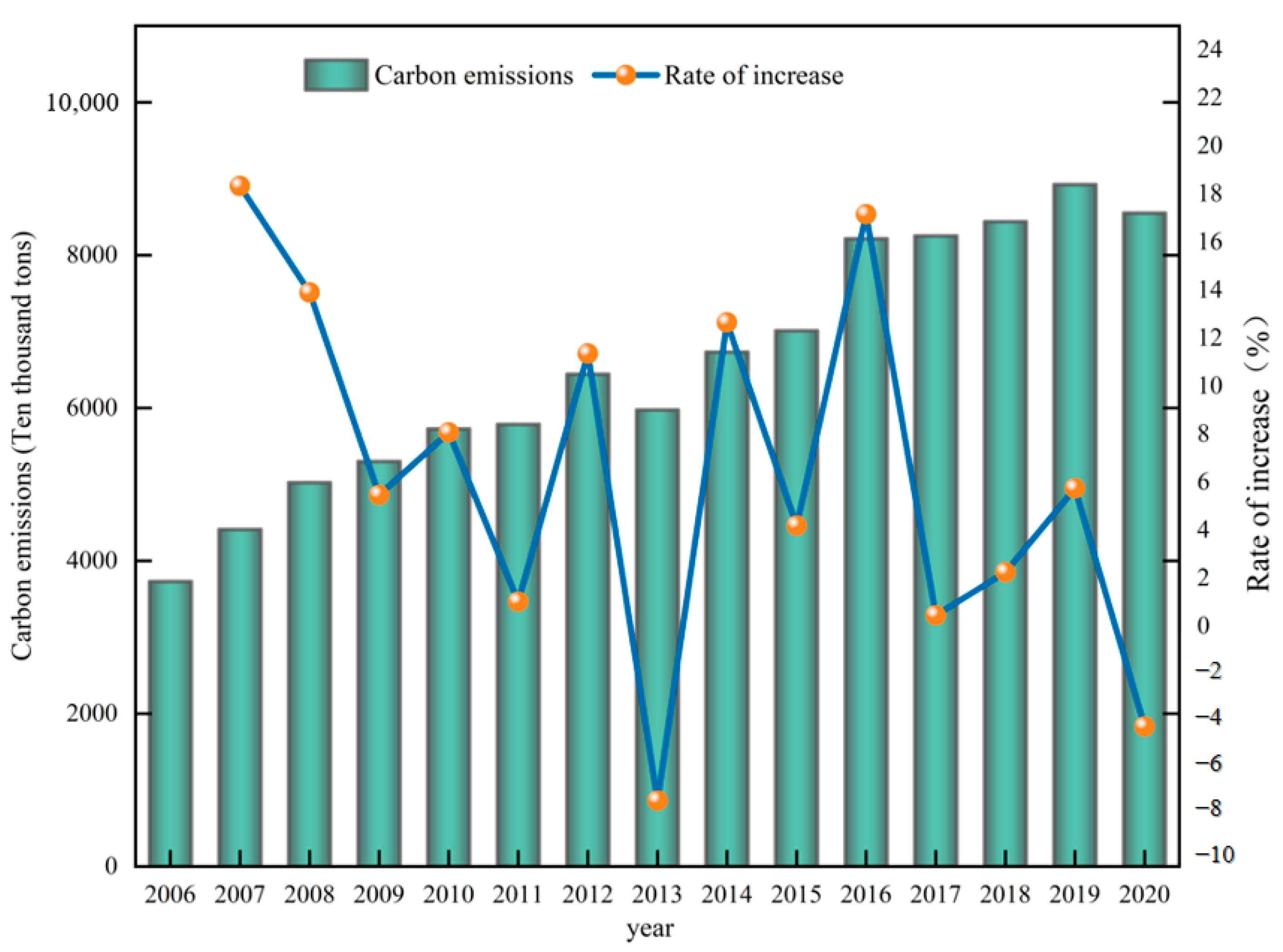
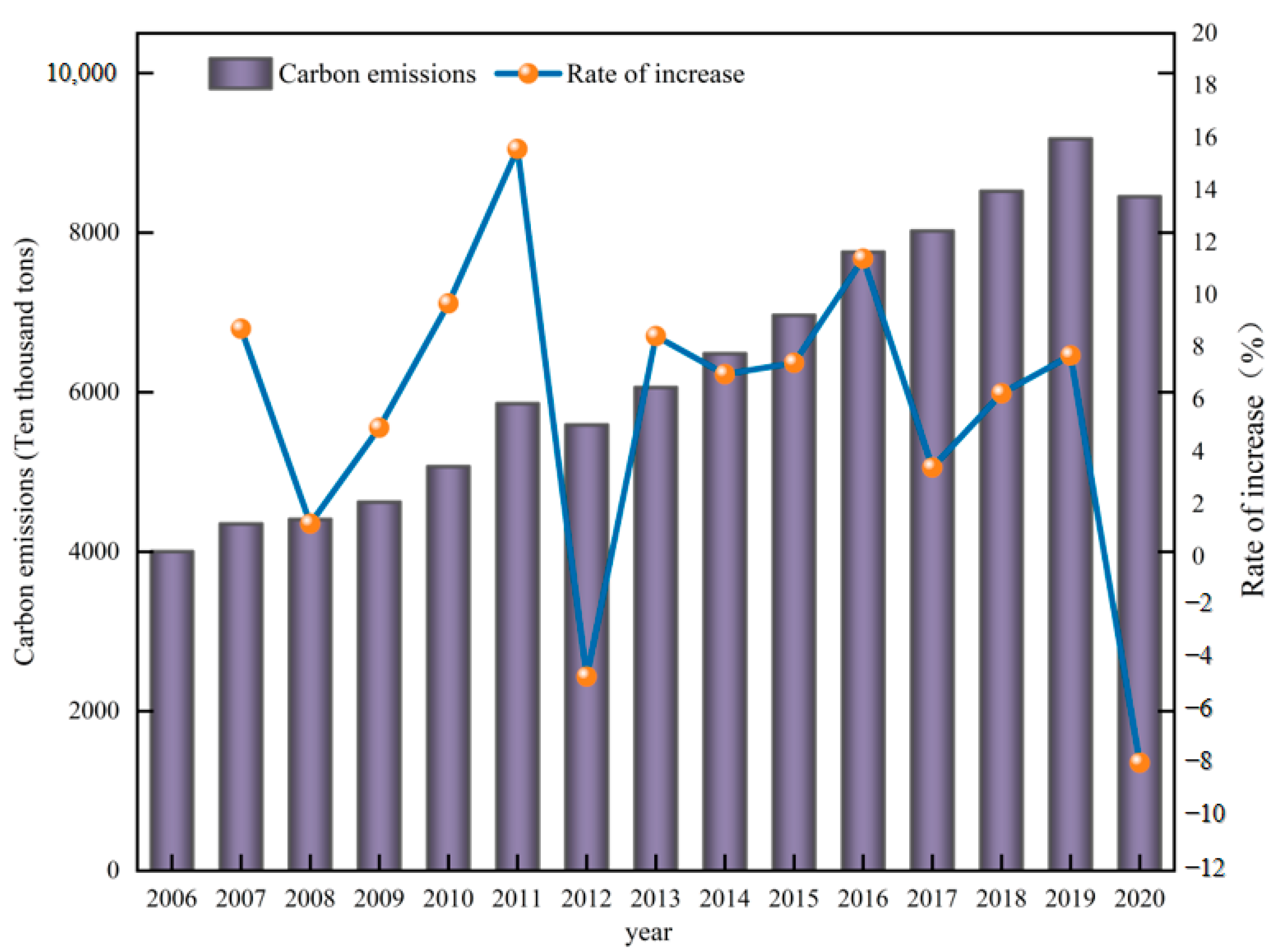
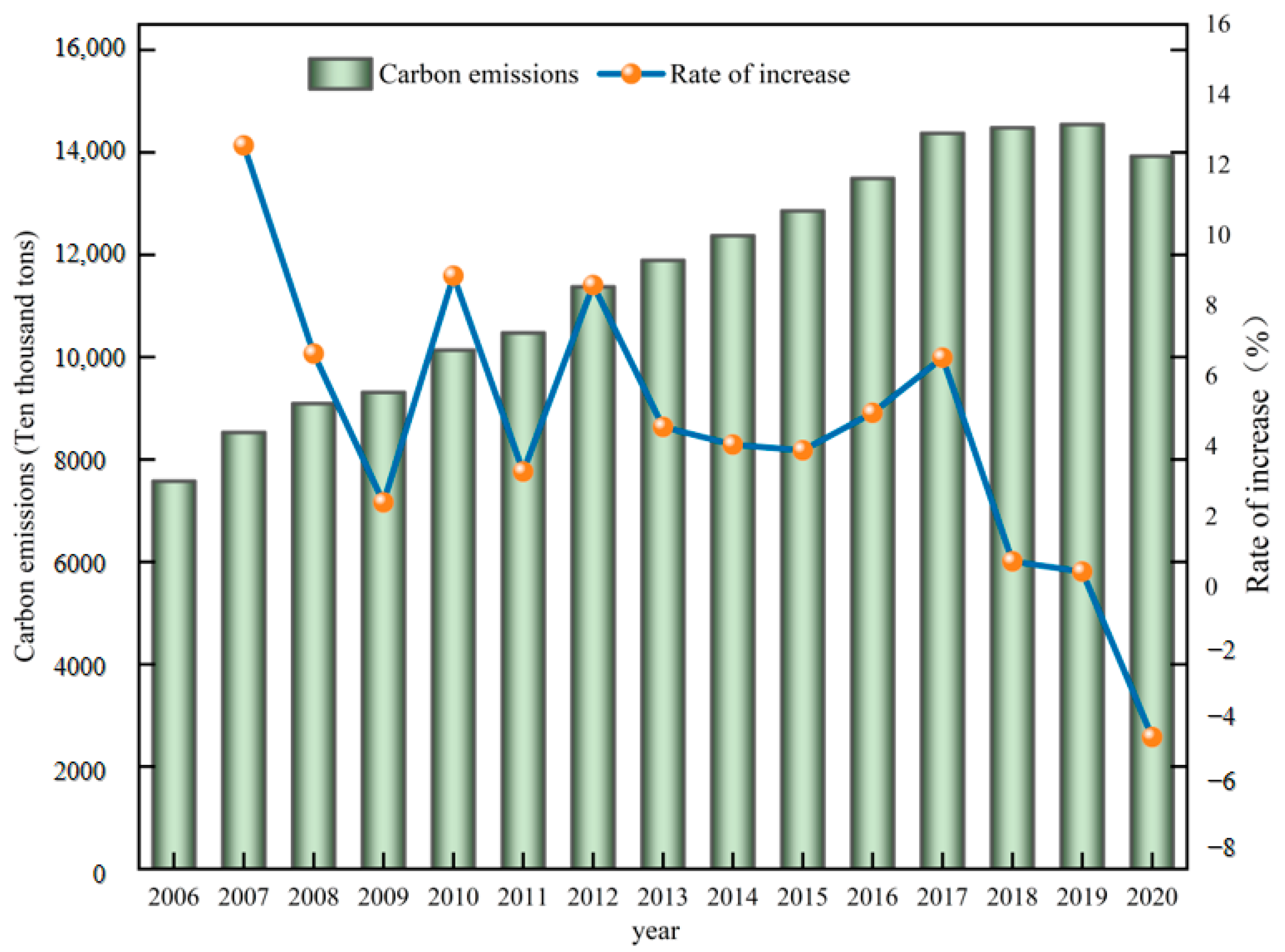
Due to the vast area of the YEB, the economic, social, and cultural characteristics of various provinces and cities are diverse and distinct, thus presenting spatial heterogeneity. Therefore, according to the official classification, this study is divided into three regions: upstream (Chongqing, Sichuan, Guizhou, and Yunnan), midstream (Jiangxi, Hubei, and Hunan), and downstream (Shanghai, Jiangsu, Zhejiang, and Anhui). This partitioning method is not only consistent with the geographical characteristics of the provinces and municipalities, but also with their administrative and economic characteristics. The results related to the changes in carbon emissions from transportation energy in the YEB from 2006 to 2020 were accounted for by the above carbon emission calculation methods, and the specific data are shown in Figure 1, Figure 2, Figure 3 and Figure 4.
The results of carbon emissions were analyzed, as follows. Regarding the overall trend, during the period 2006–2020, the total carbon emissions from energy consumption in the YEB show a fluctuating growth trend. In specific terms, the carbon emissions amounted to 153.35 million tons in 2006, and by 2020, it had escalated to 309.28 million tons, registering an average annual growth rate of 5.14%. However, the overall growth rate of carbon emissions showed a trend of fluctuation and decrease over this period. Further segmentation analysis reveals that, except for between 2019–2020, the growth rate of TCE sector has increased steadily, i.e., the growth rates reached 12.73% in 2006–2007 and 9.81% in 2015–2016. Affected by the pandemic, the major indicators of the transportation industry fluctuated considerably in 2019–2020, with significant declines in transport volumes, resulting in a corresponding reduction in energy consumption and carbon emissions, which decreased by 17.14 million tonnes in 2020 compared to 2019.
From a regional perspective: the distribution of TCE in the YEB from 2006 to 2020 shows that there are distinctive emission trends in the upstream, midstream, and downstream regions. The carbon emissions in the upstream region showed fluctuating growth in general and only showed a downward trend in 2012–2013 and 2019–2020, in which carbon emissions in 2012 decreased by about 7.26% compared to 2013. In the middle regions, except for the declining trend in 2011–2012 and 2019–2020, the remaining periods showed an increasing trend, especially during 2010–2011, when the growth rate was as high as 15.57%. The development trend of carbon emissions in the downstream region is similar to the overall emission trend of the YEB, which generally shows a fluctuating growth trend. Beyond 2019–2020, carbon emissions have grown steadily, from 75.76 million tons in 2006 to 13.925 million tons in 2020, with a total growth of 6.349 million tons and an average annual growth of 4.44%.
In conclusion, along with economic development and social progress, there has been a consistent increase in energy consumption and TCE in the YEB region. Therefore, conducting research on TCE in this area is of paramount importance for ecological environmental protection and sustainable development.

3.2. Construction of a Carbon Emission Prediction Model

3.2.1. Multicollinearity Test

A number of studies have shown that there are interactions between population, economy, and technology. There is a precise or high correlation between their data; that is, there may be a degree of co-linearity, resulting in distortion of the model estimate, thereby reducing accuracy. Therefore, this study uses SPSS 27.0 software to carry out ordinary least squares linear (OLS) regression and analyzes the multiple co-linearities between the various influencing factors in the extended STIRPAT model. The specific regression results are arranged as shown in Table 4. From the regression results, it can be observed that most of the explanatory variables exhibit VIF values greater than 10, indicating that there is a significant problem of multicollinearity among the variables.

3.2.2. Ridge Regression Analysis

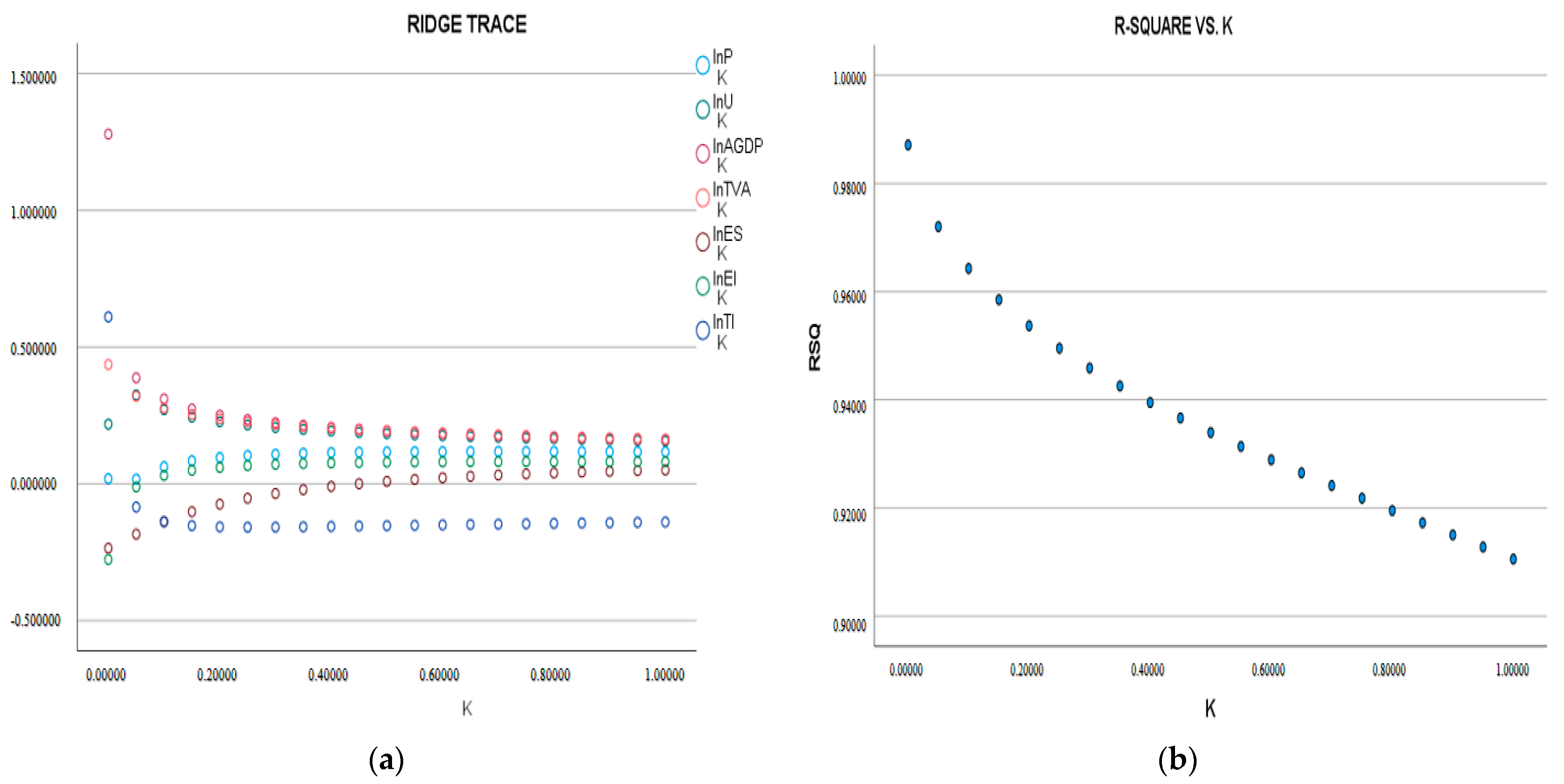
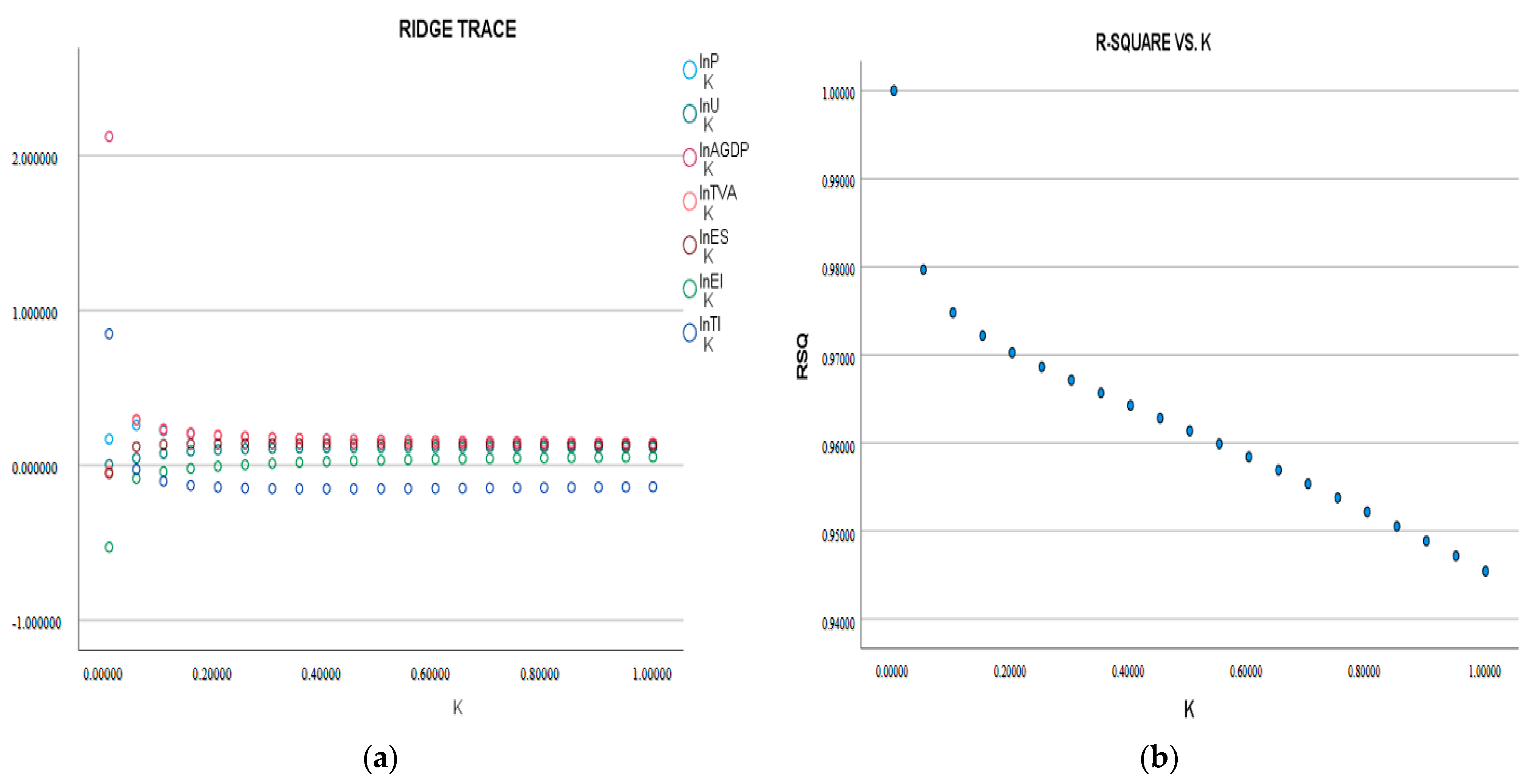
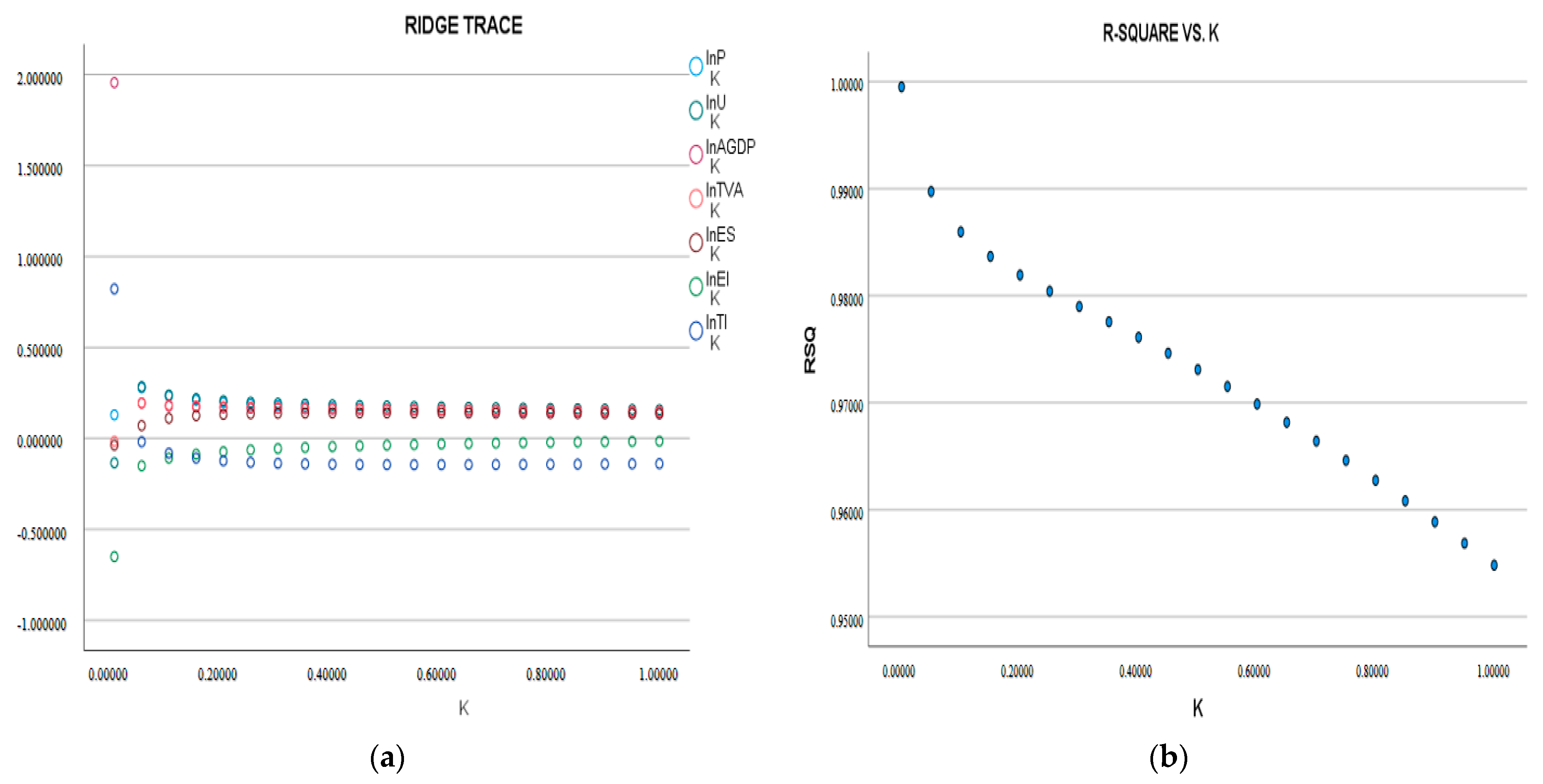
From the above analysis, it can be seen that the data series discussed in this study is not suitable for the application of ordinary least squares analysis for unbiased parameter estimation. In order to minimize the effect of multicollinearity on the estimation results and to obtain more reliable fitting results, the data are re-analyzed using the ridge regression method. Ridge regression is an improved method of OLS which limits the size of the regression coefficients by discarding the unbiased nature of the OLS and giving up part of the data information and prediction accuracy to make the estimation results closer to the reality, thus improving the reliability [33]. Due to its ability to both ameliorate the multicollinearity problem and reduce the coefficient differences between the features of interest, while not being susceptible to outliers when obtaining stable estimation results, as well as its ability to handle high-latitude datasets to avoid overfitting, ridge regression is currently widely used for covariance data analysis. By observing the ridge trace map and the change map of R2 (Figure 5, Figure 6 and Figure 7), the optimal ridge parameter K is determined, which is 0.15 in the upstream, 0.10 in the midstream, and 0.20 in the downstream regions. Based on this method, the analysis results of ridge regression are shown in Table 5.
As can be seen from ridge regression results, the R2 of the prediction model for carbon emissions from transportation in the upstream, midstream, and downstream regions of the YEB both exceeds 0.97, which indicates that the regression results are reliable, and the Sig F values are all 0.000 (less than 5%), passing the F-test, indicating that the regression equations are significant, and the model is of practical significance. The resulting extended STIRPAT models are as follows:
upstream region:
l n C = 3.17843 + 1.05714 l n P + 0.40774 l n U + 0.12926 l n A G D P + 0.13140 l n T V A 0.15681 l n E S + 0.12170 l n E I 0.19240 l n T I
Midstream region:
l n C = 37.56379 + 4.52064 l n P + 0.47867 l n U + 0.09107 l n A G D P + 0.10925 l n T V A + 0.11890 l n E S 0.15688 l n E I 0.08953 l n T I
Downstream region:
l n C = 1.83044 + 1.00646 l n P + 0.22497 l n U + 0.09361 l n A G D P + 0.10607 l n T V A + 0.08477 l n E S 0.01215 l n E I 0.16616 l n T I

3.2.3. Test of Fit Effect

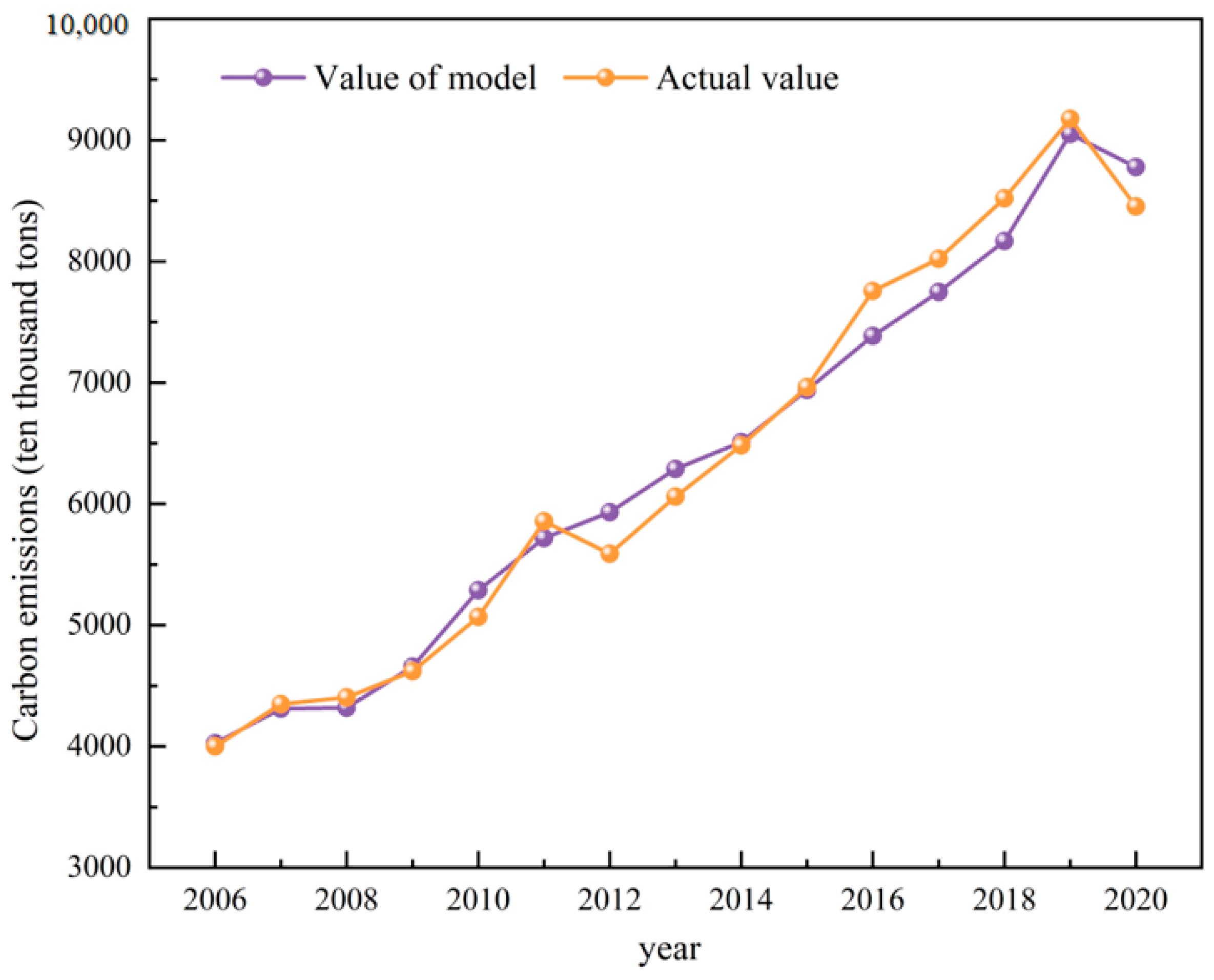
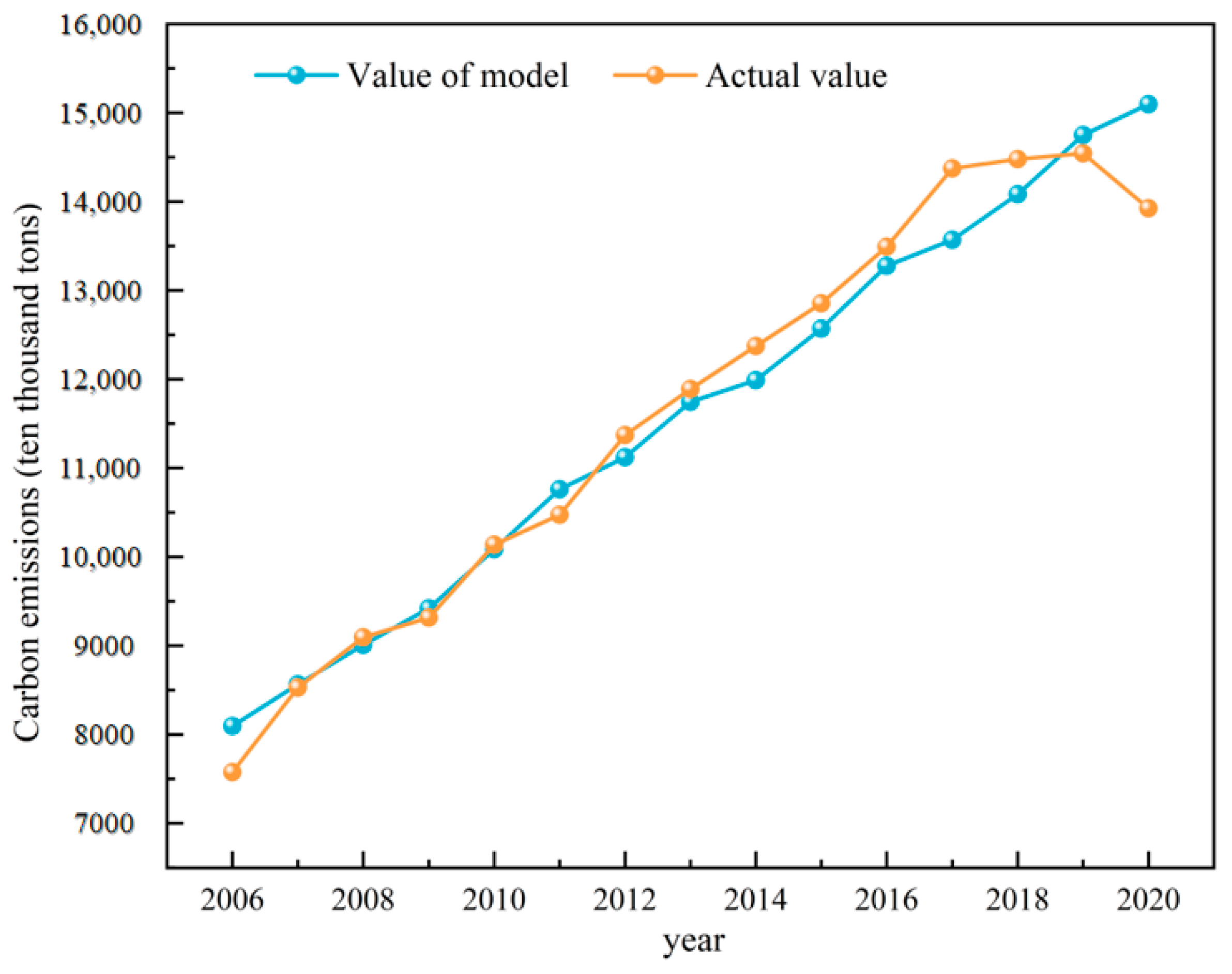
Prior to predicting and analyzing future carbon emissions, it is essential to assess the goodness-of-fit of the regression model that captures the factors influencing carbon emissions from transportation sector in the YEB. In this paper, the back-generation test method is used to fit the value of the model with the actual values from 2006 to 2020, and the results are shown in Figure 8, Figure 9 and Figure 10. The average errors of the upstream, midstream, and downstream regions are 4.23%, 2.49%, and 2.74% respectively, which are all within a reasonable range. This paper demonstrates that the prediction model developed here exhibits high accuracy and can be utilized for forecasting TCE in the area. Hence, it can be inferred that the model holds significant practical value in predicting transportation-related carbon emissions in the YEB region.

4. Projections of Peak Carbon Emissions

4.1. Scenario Analysis

The practice of scenario analysis is commonly employed to examine the future trajectory of carbon emissions. In order to ensure the accuracy of the parameter settings, this paper combines the actual situation with the relevant policy planning, based on the research of previous scholars. Based on the actual situation of the economic and social development of the YEB from 2006 to 2020, the paper summarizes the current situation in regards to development, relevant development planning, policy, and related literature, and hypothesizes the future emissions of the YEB transportation sector. The study proposes four development scenarios, namely the benchmark scenario (BM), the low-carbon scenario (LC), the strengthened low-carbon scenario (ELC), and the high-carbon scenario (HC), and is divided into three forecast intervals: 2021–2025, 2026–2030, and 2031–2035.
The benchmark scenario is guided by natural and related development policies. Under this scenario, the trends in economic development, population growth, energy consumption, and the transportation industry will continue in the current situation and will be developed, to some extent, in accordance with the relevant policy and planning directives already in place.
The low-carbon scenario is based on the benchmark scenario. While implementing regional development policies, provinces and cities have intensified the implementation of energy-saving and emission-reduction policies, and are rapidly moving towards low-carbon socio-economic development and carbon emission scenarios. Under this scenario, in order to realize the early carbon peak as the goal, the focus is on the quality of economic development and economic growth, progressing to the medium and low-speed stage, while enhancing the effectiveness of the energy system and maintaining the total energy consumption at reasonable levels.
The strengthened low-carbon scenario contemplates the completion of the 14th Five-Year Plan for the Target for Dual Control of Energy and Carbon Intensity Reduction and the achievement of the goal of peak carbon emissions by 2030. On the basis of the existing development conditions and policy measures, the scenario strives to achieve the goal of reaching the peak of carbon emissions before 2030, implementing stronger measures to conserve energy and lower emissions, and adopting extraordinary emission reduction policies and measures to significantly improve energy system efficiency and maintain total energy consumption at a low level.
The high-carbon scenario regards economic growth as the main goal, and the realization of green low-carbon goals is regulated by economic development. This scenario is was created due to the impact of the global COVID-19 pandemic, as the recent level of economic development has not been able to meet the expected development goals. Thus, under this scenario, the pursuit of economic growth will be the primary goal of future development, and energy conservation, carbon reduction, and green development goals will become secondary.
The four carbon emission projection scenarios are provided, and the reasons for their impacts are included, as follows:
(1)
P:
At present, the population of various regions in China is experiencing a growing trend. On the one hand, the YEB is an important economic development center in China, with residents earning high incomes and the area offering a large number of employment opportunities, attracting many talented individuals to come here for work. On the other hand, as living standards and medical facilities continue to improve, the average life expectancy of people continues to increase. The National Population Development Plan (2016–2030) predicts that China’s population will peak and stabilize around 2030. Most scholars also believe that China may reach its population peak around 2030 [34], and that the growth trend may decline around the population peak [35]. Therefore, it is assumed that in the preceding period, the P will remain at a stable low fertility level for a long period of time, will then experience a growth trend, reaching a peak at a certain point, and then will stabilize or even decrease slightly.
(2)
U:
From 2006 to 2020, the U in all regions of the YEB has increased year by year. On the one hand, the YEB is committed to accelerating the urbanization process and promoting rural revitalization. On the other hand, the outline of the Vision 2023 goal points out that China is in a period of rapid development, with a 30% to 70% urbanization rate, and the Development Research Center of the State Council and other institutions predict that China’s urbanization rate will reach 66% to 73% in 2030. Accordingly, it is assumed that with the sustained development of the YEB, the urbanization growth rate will gradually run out of steam.
(3)
AGDP:
The AGDP growth rate is mainly influenced by the rate of economic growth. Generally speaking, after economic development reaches a certain stage, it will gradually trend to stabilize at a low and steady growth state. The historical development of AGDP in the YEB has shown an obvious growth trend, which is due to the region’s abundant resources, superior geographical advantages, and the boosting role in China’s continuous economic growth. Therefore, it can be inferred that as the region’s economy continues to develop and the role of national policy planning deepens, AGDP will continue to grow, but the growth rate shows a downward trend.
(4)
TVA:
The TVA refers to the newly created value of transportation in the process of production and operation over a certain period of time. TVA is an important part of the gross domestic product (GDP) and reflects the development and dynamic degree of the transportation industry in a country or region. From 2006 to 2020, the GDP of the YEB continued to grow in regards to the transportation industry gross domestic product, but the average annual growth rate gradually declined, shifting from a high growth rate in 2006–2010 to a medium-high growth rate in the latter period. Therefore, it is assumed that the TVA will continue to show a declining growth rate year by year.
(5)
ES:
With the promotion of the high-quality development of the YEB, ES has changed dramatically, and the proportion of clean energy has sustained growth. At the same time, the 14th Five-Year Plan, the Dual Carbon Goals, the YEB Planning and Development Outline, and the current promotion of green transportation, low-carbon transportation, and other policies require a sustained increase in the proportion of clean energy, and they vigorously promote new energy vehicles. Therefore, it is assumed that the ES shows an increasing trend, but the growth rate will decrease with each passing year.
(6)
EI:
The EI indicates the energy consumption per unit turnover and serves as an indicator of the efficiency of energy-saving and emission-reduction technologies. As the level of these technologies reaches a marginal effect, the difficulty of carbon reduction is gradually increased, with the decline in the rate of energy consumption per unit of turnover gradually slowing down. On the one hand, the Outline of the Planning and Development of the YEB and the Overview of China’s Transportation Energy Conservation and Emission Reduction Related Data and Key Standards and Regulations requires a decrease in energy consumption per unit of turnover. On the other hand, according to the guidance of the 14th Five-Year Plan, China is currently facing many difficulties and challenges in regards to emission reduction. Therefore, it is assumed that the EI is transitioning from the rapid decline stage to the medium-high decline stage and an overall negative growth trend.
(7)
TI:
As a basic indicator to evaluate the development level of the transportation industry, a decline in TI value can reduce ineffective conveyance in the transportation process, enhancing the organizational management technology level and the efficiency of the transportation industry. The outline proposes to improve the comprehensive transport pattern, speed up the construction of a modern comprehensive transport system, and support relevant policies required to improve transport efficiency and optimize the transport system. Therefore, it is assumed that as the transportation system and infrastructure are consistently optimized and enhanced, transport efficiency will continue to improve, and the TI will gradually decrease.
In summary, the growth rate settings of the model-related parameters, under different scenarios and in different regions of the YEB from 2031 to 2035, are shown in Table 6.

4.2. Analysis of Prediction Results

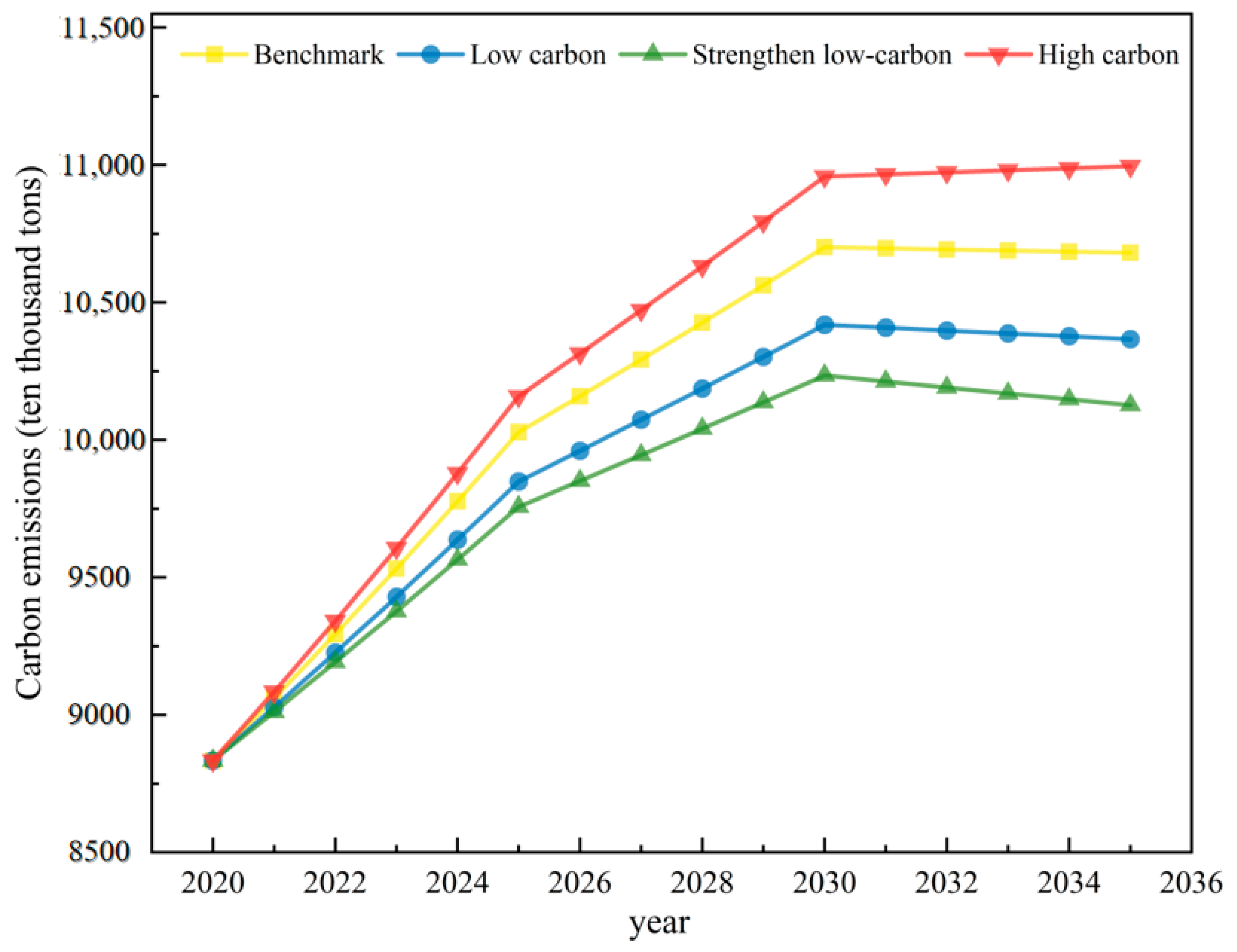
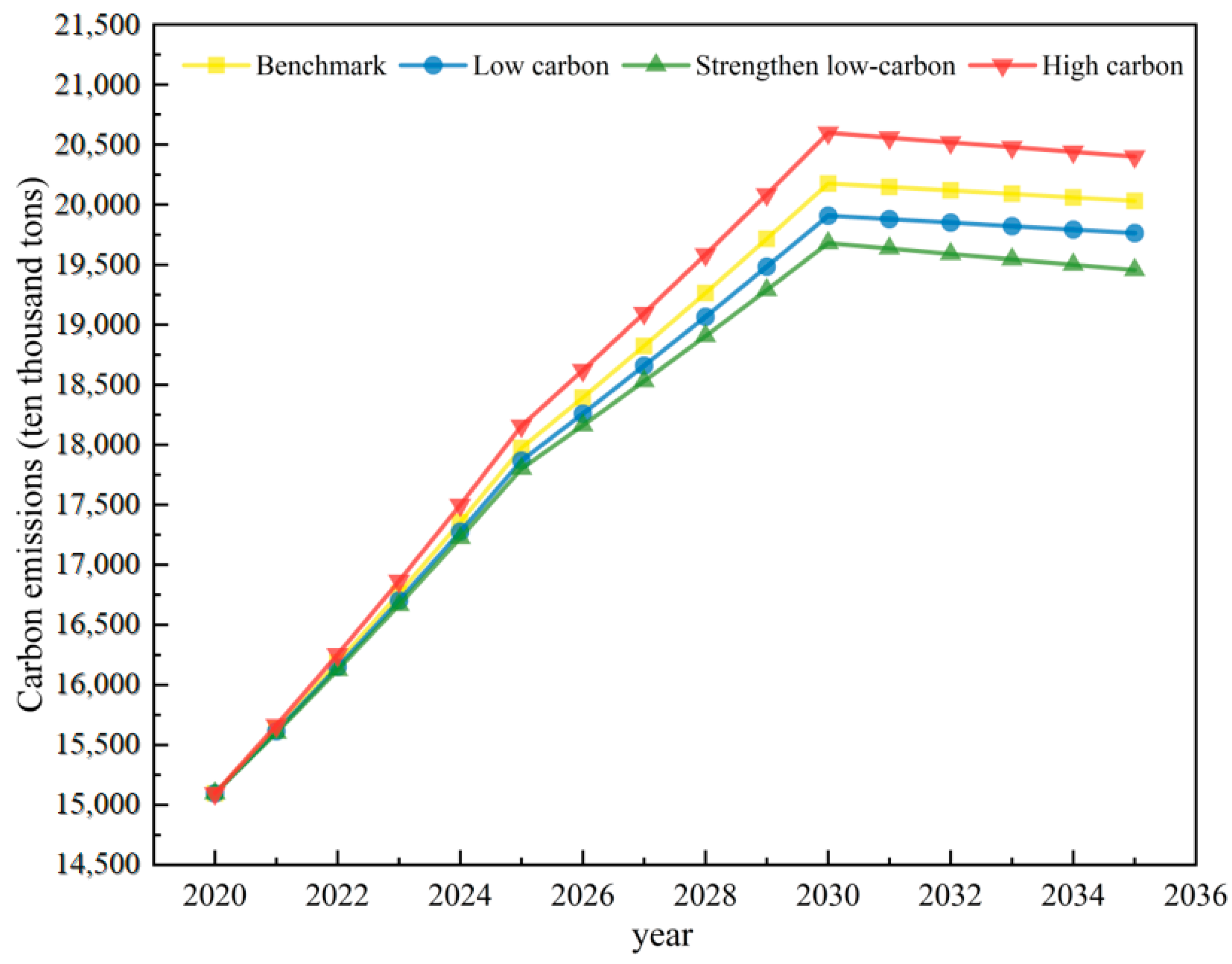
According to different scenarios combined with the constructed extended STIRPAT model, the carbon emissions from transportation in the YEB from 2021 to 2035 are predicted. The results of each scenario are shown in Figure 11, Figure 12 and Figure 13.
According to the projected results, there are significant variations in transportation-related carbon emissions across different regions of the YEB under various scenarios, with differing peak levels and carbon emissions. In the upstream region, carbon emissions resulting from transportation under the BM, LC, and ELC scenarios are projected to peak in 2030, followed by slow declines at different rates. In the HC scenario, TCE will not peak in 2030 and will show a low growth trend after that because these provinces and cities focus more on economic growth rather than green, low-carbon, and high-quality development. In the midstream region, the forecast shows that transport carbon emissions will peak in 2030 under all scenarios, with a peak of 136.2 million tons in the BM scenario, 134.57 million tons in the LC scenario, 133.13 million tons in the ELC scenario, and 138.73 million tons in the HC scenario. Therefore, it is predicted that the development of the midstream region is expected to achieve the national targets of peaking carbon emissions by 2030 and carbon neutrality by 2060. In the downstream region, the projections show that all scenarios are able to reach peak carbon emissions by 2030. This is due to the economic prosperity of the downstream cities, the relative prosperity of the residents, and the high degree of advanced modernization, which are the key pilot factors in the important development planning policies for many countries. Therefore, it is predicted that the downstream provinces and municipalities will be able to meet the 14th Five-Year Plan and the national “double carbon” target. In summary, it is predicted that except for the upstream HC scenario, other regions are expected to reach the peak of carbon emissions in 2030 under all scenarios. Therefore, for the sake of realizing the overall peak of carbon emissions in the YEB, it is necessary to focus on the regulation of the upstream region to technically reduce total emissions and carbon emissions.

5. Conclusions and Recommendations

5.1. Conclusions

The primary findings derived from this study are as follows:
(1)
From 2006 to 2019, the TCE in the YEB showed a fluctuating growth trend and decreased slightly in 2020. Ranking the carbon emissions of the regions in descending order, the downstream is the highest, the midstream the second, and the upstream the lowest, a phenomenon that is mainly associated with the level of development of each region.
(2)
Each influencing factor exhibited different impacts on TCE in different regions. P, U, AGDP, and TVA all contributed to an increase in carbon emissions in the upstream, midstream, and downstream regions. In terms of technology, each factor showed a different level of influence, i.e., the upstream region is mainly affected by TI, the midstream region by EI, and the downstream region by TI.
(3)
Under different scenarios, there are significant differences in the carbon peak condition of the transport industry in different regions, not only in terms of peak carbon emissions, but also in terms of peak time. To better realize the requirements of the 14th Five-Year Plan and to achieve the “double carbon” goals, adopting a low-carbon scenario or a strengthened low-carbon scenario may be more in line with the future development trend.

5.2. Recommendations

This paper proposes the following recommendations to mitigate the growth of carbon emissions from transportation in the YEB:
(1)
Promote the organic integration of urban development with the construction of low-carbon cities and transportation.
This can be achieved by appropriately increasing financial support for the construction of new low-carbon cities, using low-carbon and environmentally friendly materials to build roads, and reducing carbon emissions during road construction and maintenance. The rational planning of the layout of cities to promote the balanced distribution of residential, commercial, and industrial areas and to reduce commuting distances should also be employed. Relevant laws should be formulated to mandate emission standards and low-carbon requirements for public transportation, guiding enterprises and citizens to participate in the construction of low-carbon transportation through taxation, subsidies, and other policy instruments. At the same time, according to the different foundations and advantages in each region of opening up to the outside world, the level of open economy development should be upgraded according to local conditions in order to realize a win–win situation beneficial to both economic development and ecological and environmental protection.
(2)
Enhance the utilization of clean energy and the optimize the pattern of energy consumption.
The electrification of vehicles should be encouraged by promoting new means of transportation such as electric vehicles, hybrid vehicles, hybrid ships, and hybrid trains, increasing subsidies for new energy vehicles, and building more charging piles and power exchange stations. The public transportation system should be optimized, encourage non-motorized travel and gradually reducing the use of traditional fuel vehicles. Meanwhile, the use of biofuels, hydrogen energy, and other clean energy sources can also be explored to replace traditional fuels and promote the formation of a low-carbon, scientific, and rational pattern of diversified energy consumption.
(3)
Improve the efficacy of energy-saving technology and reduce energy intensity.
Regional governments should actively promote cooperation among scientific research institutions, enterprises, and institutions of higher education to jointly carry out research and development in regards to energy-saving technologies and actively push the transformation and application of scientific and technological achievements. In this process, they should focus on energy utilization and clean energy research and development, strengthen the studies and promotion of new energy technologies, and strive to raise energy utilization efficiency.
(4)
Develop smart transportation and improve transport efficiency.
The construction of new types of infrastructure, like smart highways, railroads, ports, waterways, and hubs, should be enhanced, and the in-depth fusion of cutting-edge technologies, such as 5G and artificial intelligence, should be accelerated within the field of transportation. Self-driving buses and cabs, as well as vehicle–road coordination technologies, should be promoted to reduce traffic accidents and improve road usage efficiency. Intelligent traffic signal systems should also be applied to adjust signals based on real-time traffic flow to reduce traffic congestion and carbon emissions.
At the same time, each region should strengthen all aspects of carbon emissions reduction work, according to its own actual situation in compliance with local conditions. Upstream regions can rely on resource advantages to develop low-carbon industries; to strengthen the informatization construction of railroad transportation; to use technologies, such as big data and the Internet of things, to improve the efficiency and management level of transportation; to promote transport integration and convergence; and to promote the construction of logistics information platforms to achieve the sharing and optimization of logistics information. The midstream region can give full play to its industrial advantages, upgrading the industrial chain and fostering the enhancement and upgrading of its industrial structure. It can also use these advantages to strengthen the construction of transportation infrastructure; to raise the quality of and standards for roads, bridges, and other transportation facilities; and to develop smart ports, promote the intelligent transformation of established ports, and improve the operational efficiency and service level of these ports. Downstream areas, on the other hand, can make full use of the advantages of their location by expanding their current opening up to the outside world, attracting foreign investment, introducing advanced technology and management experience, and enhancing international competitiveness. This region can also focus on the advancement of intelligent waterborne transportation systems to enhance the communication and convenience of waterborne transportation and promote intelligent public transportation systems to reduce traffic congestion.

Author Contributions

Conceptualization, Y.S. and G.Z.; methodology, Y.S.; software, G.Z.; validation, Y.S. and G.Z.; formal analysis, Y.S.; investigation, Y.S.; resources, Y.S. and G.Z.; data curation, G.Z.; writing—original draft preparation, Y.S.; writing—review and editing, Y.S. and G.Z.; visualization, Y.S. and G.Z.; supervision, Y.S.; project administration, Y.S.; funding acquisition, Y.S. All authors have read and agreed to the published version of the manuscript.

Funding

This research received no external funding.

Data Availability Statement

Restrictions apply to the availability of these data. Data was obtained from China Statistics Bureau and are available China Statistics Bureau with the permission of China Statistics Bureau.

Conflicts of Interest

The authors declare no conflict of interest.

References

  1. Zhang, Y.; Li, X.; Zhang, Y. A novel integrated optimization model for carbon emission prediction: A case study on the group of 20. J. Environ. Manag. 2023, 344, 118422. [Google Scholar] [CrossRef] [PubMed]
  2. Miao, L. Examining the impact factors of urban residential energy consumption and CO2 emissions in China—Evidence from city-level data. Ecol. Indic. 2017, 73, 29–37. [Google Scholar] [CrossRef]
  3. Li, J.; Lin, B. Does energy and CO2 emissions performance of China benefit from regional integration? Energy Policy 2017, 101, 366–378. [Google Scholar] [CrossRef] [PubMed]
  4. Chen, X.; Shuai, C.; Wu, Y.; Zhang, Y. Analysis on the carbon emission peaks of China’s industrial, building, transport, and agricultural sectors. Sci. Total Environ. 2020, 709, 135768. [Google Scholar] [CrossRef]
  5. Li, F.; Cai, B.; Ye, Z.; Wang, Z.; Zhang, W.; Zhou, P.; Chen, J. Changing patterns and determinants of transportation carbon emissions in Chinese cities. Energy 2019, 174, 562–575. [Google Scholar] [CrossRef]
  6. Wang, Y.; Xie, T.; Yang, S. Carbon emission and its decoupling research of transportation in Jiangsu Province. J. Clean. Prod. 2017, 142, 907–914. [Google Scholar] [CrossRef]
  7. Bai, C.; Chen, Z.; Wang, D. Transportation carbon emission reduction potential and mitigation strategy in China. Sci. Total Environ. 2023, 873, 162074. [Google Scholar] [CrossRef]
  8. Zhang, Y.; Sun, M.; Yang, R.; Li, X.; Zhang, L.; Li, M. Decoupling water environment pressures from economic growth in the Yangtze River Economic Belt, China. Ecol. Indic. 2021, 122, 107314. [Google Scholar] [CrossRef]
  9. Li, D.; Zhang, J. Measurement and analysis of ecological pressure due to industrial development in the Yangtze River economic belt from 2010 to 2018. J. Clean. Prod. 2022, 353, 131614. [Google Scholar] [CrossRef]
  10. Wang, Y.; Zhou, Y.; Zhu, L.; Zhang, F.; Zhang, Y. Influencing Factors and Decoupling Elasticity of China’s Transportation Carbon Emissions: 5. Energies 2018, 11, 1157. [Google Scholar] [CrossRef]
  11. Sun, Y.; Liu, S.; Li, L. Grey Correlation Analysis of Transportation Carbon Emissions under the Background of Carbon Peak and Carbon Neutrality: 9. Energies 2022, 15, 3064. [Google Scholar] [CrossRef]
  12. Solís, J.C.; Sheinbaum, C. Energy consumption and greenhouse gas emission trends in Mexican road transport. Energy Sustain. Dev. 2013, 17, 280–287. [Google Scholar] [CrossRef]
  13. Alam, M.S.; Hyde, B.; Duffy, P.; McNabola, A. Assessment of pathways to reduce CO2 emissions from passenger car fleets: Case study in Ireland. Appl. Energy 2017, 189, 283–300. [Google Scholar] [CrossRef]
  14. González Palencia, J.C.; Otsuka, Y.; Araki, M.; Shiga, S. Scenario analysis of lightweight and electric-drive vehicle market penetration in the long-term and impact on the light-duty vehicle fleet. Appl. Energy 2017, 204, 1444–1462. [Google Scholar] [CrossRef]
  15. Cai, B.; Cao, L.; Lei, Y.; Wang, C.; Zhang, L.; Zhu, J.; Li, M.; Du, M.; Lv, C.; Jiang, H.; et al. China’s carbon emission pathway under the carbon neutrality target. China Popul. Resour. Environ. 2021, 31, 7–14. [Google Scholar]
  16. Xu, B.; Lin, B. Differences in regional emissions in China’s transport sector: Determinants and reduction strategies. Energy 2016, 95, 459–470. [Google Scholar] [CrossRef]
  17. Xie, R.; Fang, J.; Liu, C. The effects of transportation infrastructure on urban carbon emissions. Appl. Energy 2017, 196, 199–207. [Google Scholar] [CrossRef]
  18. Yang, S.; Cao, D.; Lo, K. Analyzing and optimizing the impact of economic restructuring on Shanghai’s carbon emissions using STIRPAT and NSG-Ⅱ. Sustain. Cities Soc. 2018, 40, 44–53. [Google Scholar] [CrossRef]
  19. Li, Y.; Du, Q.; Lu, X.; Wu, J.; Han, X. Relationship between the development and CO2 emissions of transport sector in China. Transp. Res. Part D Transp. Environ. 2019, 74, 1–14. [Google Scholar] [CrossRef]
  20. Solaymani, S. CO2 emissions patterns in 7 top carbon emitter economies: The case of transport sector. Energy 2019, 168, 989–1001. [Google Scholar] [CrossRef]
  21. Bai, C.; Du, K.; Yu, Y.; Feng, C. Understanding the trend of total factor carbon productivity in the world: Insights from convergence analysis. Energy Econ. 2019, 81, 698–708. [Google Scholar] [CrossRef]
  22. Wang, S.; Li, J.; Zhao, E. Pathways to achieve low-carbon transition in the transportation sector under the constraints of carbon peak and carbon neutrality targets: A comprehensive analysis of intra- and extra-industry factors. Sustain. Energy Technol. Assess. 2023, 60, 103490. [Google Scholar] [CrossRef]
  23. Xiao, Y.; Ma, D.; Zhang, F.; Zhao, N.; Wang, L.; Guo, Z.; Zhang, J.; An, B.; Xiao, Y. Spatiotemporal differentiation of carbon emission efficiency and influencing factors: From the perspective of 136 countries. Sci. Total Environ. 2023, 879, 163032. [Google Scholar] [CrossRef] [PubMed]
  24. Wu, L.; Liu, S.; Liu, D.; Fang, Z.; Xu, H. Modelling and forecasting CO2 emissions in the BRICS (Brazil, Russia, India, China, and South Africa) countries using a novel multi-variable grey model. Energy 2015, 79, 489–495. [Google Scholar] [CrossRef]
  25. Li, Q.; Zhang, W.; Li, H.; He, P. CO2 emission trends of China’s primary aluminum industry: A scenario analysis using system dynamics model. Energy Policy 2017, 105, 225–235. [Google Scholar] [CrossRef]
  26. Wu, C.B.; Huang, G.H.; Xin, B.G.; Chen, J.K. Scenario analysis of carbon emissions’ anti-driving effect on Qingdao’s energy structure adjustment with an optimization model, Part I: Carbon emissions peak value prediction. J. Clean. Prod. 2018, 172, 466–474. [Google Scholar] [CrossRef]
  27. Fang, Y.; Lu, X.; Li, H. A random forest-based model for the prediction of construction-stage carbon emissions at the early design stage. J. Clean. Prod. 2021, 328, 129657. [Google Scholar] [CrossRef]
  28. Gao, M.; Yang, H.; Xiao, Q.; Goh, M. A novel fractional grey Riccati model for carbon emission prediction. J. Clean. Prod. 2021, 282, 124471. [Google Scholar] [CrossRef]
  29. Liu, Z.; Jiang, P.; Wang, J.; Zhang, L. Ensemble system for short term carbon dioxide emissions forecasting based on multi-objective tangent search algorithm. J. Environ. Manag. 2022, 302, 113951. [Google Scholar] [CrossRef]
  30. Ehrlich, P.R.; Holdren, J.P. Impact of Population Growth: Complacency concerning this component of man’s predicament is unjustified and counterproductive. Science 1971, 171, 1212–1217. [Google Scholar] [CrossRef]
  31. York, R.; Rosa, E.A.; Dietz, T. STIRPAT, IPAT and ImPACT: Analytic tools for unpacking the driving forces of environmental impacts. Ecol. Econ. 2003, 46, 351–365. [Google Scholar] [CrossRef]
  32. Sun, Y.; Yang, Y.; Liu, S.; Li, Q. Research on Transportation Carbon Emission Peak Prediction and Judgment System in China. Sustainability 2023, 15, 14880. [Google Scholar] [CrossRef]
  33. Qian, Y.; Sun, L.; Qiu, Q.; Tang, L.; Shang, X.; Lu, C. Analysis of CO2 Drivers and Emissions Forecast in a Typical Industry-Oriented County: Changxing County, China. Energies 2020, 13, 1212. [Google Scholar] [CrossRef]
  34. Zhang, X.; Zhai, Z.; Tao, T. Trends and Patterns of Negative Population Growth in China. Popul. Res. 2020, 44, 3–20. [Google Scholar]
  35. Lin, N. The influence of the downward tendency of the gross labor force on long-term competitiveness of major countries—An International comparative study on the UN World Population Prospects (2017). Macroecon. Manag. 2019, 3, 31–37. [Google Scholar]
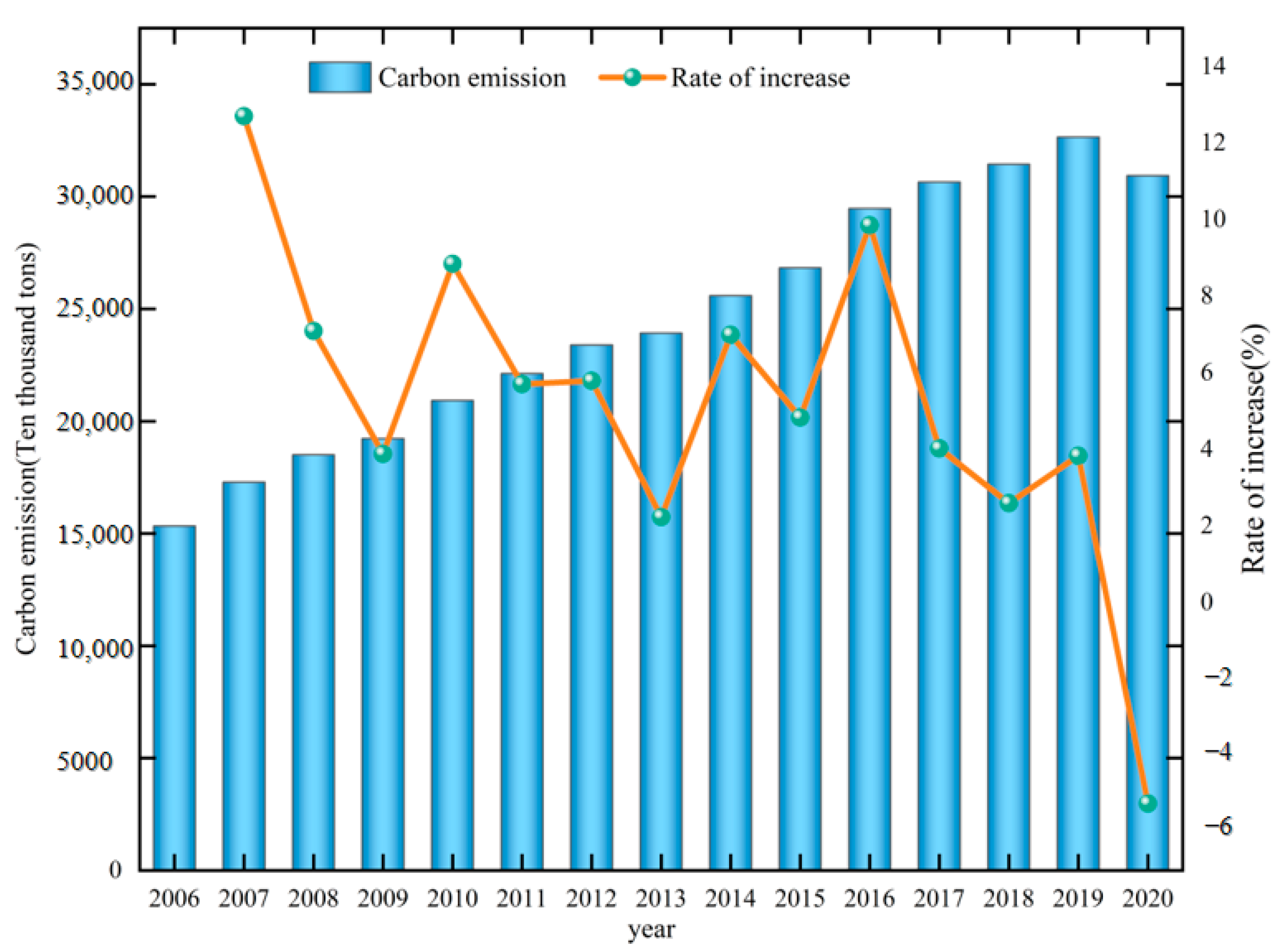
Figure 1. Carbon emissions of YEB.
Energies 17 03364 g001
Figure 2. Carbon emissions of upstream region.
Energies 17 03364 g002
Figure 3. Carbon emissions of midstream region.
Energies 17 03364 g003
Figure 4. Carbon emissions of downstream region.
Energies 17 03364 g004
Figure 5. Ridge regression results for the upstream region. (a) ridge trace; (b) R-squared vs. K.
Energies 17 03364 g005
Figure 6. Ridge regression results for the midstream region. (a) ridge trace; (b) R-squared vs. K.
Energies 17 03364 g006
Figure 7. Ridge regression results for the downstream region. (a) ridge trace; (b) R-squared vs. K.
Energies 17 03364 g007
Figure 8. The fitting results for upstream region.
Energies 17 03364 g008
Figure 9. The fitting results for the midstream region.
Energies 17 03364 g009
Figure 10. The fitting results for the downstream region.
Energies 17 03364 g010
Figure 11. Predicted results for the upstream region.
Energies 17 03364 g011
Figure 12. Predicted results for the midstream region.
Energies 17 03364 g012
Figure 13. Predicted results for the downstream region.
Energies 17 03364 g013
Table 1. Model variable description.
CharacteristicVariantDescription and Calculation Method
IC (CO2 emissions)CO2 emissions from transportation energy consumption
PP (population size)Regional population
PU (urbanization rate)Urban population as a percentage of total population
AAGDP (GDP per capita)Ratio of gross regional product to population size
ATVA (transportation added value)Gross product of the transportation sector
TES (energy structure)Share of clean energy consumption in total energy consumption (including natural gas and electricity)
TEI (energy intensity)Ratio of transportation turnover to energy consumption
TTI (transportation intensity)Ratio of transportation turnover to GDP
Table 2. Carbon emission coefficient for each type of energy consumption.
Energy TypeNet Calorific Value (kJ/kg)Carbon Content per Unit of Calorific Value (t-C/TJ)Carbon Oxidation Rate (%)Carbon Emission Coefficient (kgCO2/kg)Reduced Standard Coal Coefficient (kgce/kg)
Raw coal20,90826.37941.90030.7143
Coke28,43529.42932.85270.9714
Gasoline43,07018.90982.92511.4714
Kerosene43,07019.50983.01791.4714
Diesel oil42,65220.20983.09591.4571
Fuel Oil41,81621.10983.17051.4286
Liquefied petroleum gas50,17917.20983.10131.7143
Natural gas38,93115.32992.16501.3300
Table 3. Passenger–cargo conversion coefficient.
Mode of TransportHighwayWaterwayRailway
Passenger and cargo conversion factor0.10.331
Table 4. Results of ordinary least squares analysis.
RegionVariantBStandard ErrorBetaTSig.VIF
UpstreamConstant−0.49633.031−0.0150.988
lnP0.2363.6470.0190.0650.9545.561
lnU0.3641.2750.2190.2860.783317.824
lnAGDP0.6030.3941.2791.5330.169377.246
lnTVA0.2250.2560.4360.8810.408133.254
lnES−0.3640.182−0.236−1.9980.0867.541
lnEI−0.6810.289−0.277−2.3550.0517.477
lnTI0.7700.4060.6101.8950.10056.273
MidstreamConstant−19.38323.217−0.8350.431
lnP2.5212.3790.1301.060.324218.380
lnU−0.270.415−0.134−0.6490.537620.513
lnAGDP1.0020.1791.9565.608<0.0011765.983
lnTVA−0.0090.071−0.016−0.1300.900208.486
lnES−0.0390.116−0.037−0.3400.744170.884
lnEI−0.940.141−0.650−6.681<0.001137.368
lnTI0.9060.1750.8225.1760.001365.768
DownstreamConstant−4.9100.823−5.964<0.001
lnP0.8810.0830.17010.644<0.001187.120
lnU0.0130.0180.0060.7210.49547.166
lnAGDP1.0300.0122.12287.515<0.001430.171
lnTVA−0.0220.013−0.040−1.7110.131406.817
lnES−0.0310.015−0.052−2.1180.072441.346
lnEI−1.0060.015−0.528−67.850<0.00144.270
lnTI1.0070.0160.85062.407<0.001135.618
Table 5. Results of ridge regression analysis.
RegionR2VariantBStandard ErrorBetaT ValueF Value
Upstream0.979constant−3.178439.347720.00000−0.3400223.096
LnP1.057140.946320.084001.11711
LnU0.407740.066670.244766.11545
LnAGDP0.129260.021610.273865.98198
LnTVA0.131400.024040.254565.46511
LnES−0.156810.13987−0.10154−1.12111
LnEI0.121700.177100.049450.68720
LnTI−0.192400.07173−0.15258−2.68235
Midstream0.993constant−37.563799.587050.00000−3.9181870.238
LnP4.520640.983580.233164.59612
LnU0.478670.076490.238246.25802
LnAGDP0.091070.011310.177848.05492
LnTVA0.109250.017920.184246.09530
LnES0.118900.044140.111492.69396
LnEI−0.156880.06375−0.10854−2.46086
LnTI−0.089530.05153−0.08122−1.73760
Downstream0.985constant−1.830441.408040.00000−1.3000032.627
LnP1.006460.146060.194406.89068
LnU0.224970.090380.100932.48923
LnAGDP0.093610.009440.192959.92000
LnTVA0.106070.013700.197257.74396
LnES0.084770.011610.140207.30097
LnEI−0.012150.11026−0.00637−0.11018
LnTI−0.166160.05056−0.14024−3.28621
Table 6. Growth rate settings of influencing factors under different modes (%).
RegionScenarioForecast IntervalsPUAGDPTVAESEITI
UpstreamBM2021–20250.332.588.307.807.76−3.09−3.50
2026–20300.141.186.305.806.76−2.59−2.50
2031–2035−0.400.354.504.306.16−1.89−1.50
LC2021–20250.282.287.307.308.76−3.59−4.50
2026–20300.120.985.805.807.76−3.09−3.50
2031–2035−0.400.453.504.306.76−2.59−2.50
SLC2021–20250.262.186.806.809.76−4.09−5.50
2026–20300.120.885.305.308.76−3.59−4.50
2031–2035−0.400.453.203.807.76−3.09−3.50
HC2021–20250.382.789.308.306.76−3.09−2.50
2026–20300.181.287.306.305.76−2.59−1.50
2031–2035−0.350.355.504.305.16−2.09−0.50
MidstreamBM2021–20250.302.036.006.893.32−4.91−7.30
2026–20300.130.854.504.892.82−3.91−5.30
2031–2035−0.35−0.853.252.892.32−2.91−3.30
LC2021–20250.201.835.505.894.32−6.91−8.30
2026–20300.050.654.004.393.82−5.41−6.30
2031–2035−0.40−0.852.752.893.32−3.91−4.30
SLC2021–20250.101.635.007.395.39−7.91−9.30
2026–2030−0.050.553.505.393.89−6.41−7.30
2031–2035−0.40−0.852.251.392.89−4.91−5.30
HC2021–20250.402.237.007.892.82−3.91−5.30
2026–20300.171.035.505.892.32−2.91−3.30
2031–2035−0.30−0.853.503.391.82−1.91−2.30
DownstreamBM2021–20250.631.108.736.206.50−4.00−3.58
2026–20300.230.426.735.205.50−3.00−2.08
2031–2035−1.20−1.304.734.203.50−2.00−1.08
LC2021–20250.430.907.735.707.50−5.00−4.58
2026–20300.130.205.734.706.00−4.00−2.58
2031–2035−1.20−1.303.733.704.00−3.00−1.58
SLC2021–20250.330.807.235.208.00−6.00−5.08
2026–20300.030.155.234.206.50−5.00−2.58
2031–2035−1.20−1.303.233.204.00−4.00−1.58
HC2021–20250.731.207.739.735.50−3.00−3.08
2026–20300.330.426.737.234.50−2.00−2.08
2031–2035−1.20−1.303.734.733.50−1.00−1.08
Disclaimer/Publisher’s Note: The statements, opinions and data contained in all publications are solely those of the individual author(s) and contributor(s) and not of MDPI and/or the editor(s). MDPI and/or the editor(s) disclaim responsibility for any injury to people or property resulting from any ideas, methods, instructions or products referred to in the content.