Abstract
Currently, most studies on the optimization of wind farm layouts on flat terrain employ a discrete grid-based arrangement method and result in irregular layouts that may damage the visual appeal of wind farms. To meet the practical requirements of wind farms, a two-step optimization method called “grid–coordinate” based on a genetic algorithm is proposed in this paper. The core idea is to initially determine the number of wind turbines and their initial positions using a grid-based approach, followed by a fine-tuning of the wind farm layout by moving the turbines in a row/column manner. This two-step process not only achieves an aesthetically pleasing arrangement but also maximizes power generation. This algorithm is conducted to optimize a 2 km × 2 km wind farm under three classic wind conditions, one improved wind condition, and a real wind condition employing both the Jensen and Gaussian wake models. To validate the effectiveness of the proposed method, the optimization of configurations based on different wake models was conducted, yielding results including the efficiency, total power output, number of wind turbines, and unit cost of electricity generation. These results were compared and analyzed against the classical literature. The findings indicate that the unit cost of electricity generation using the two-step optimization approach with the Gaussian wake model is higher than that of the initial grid optimization method. Additionally, varying the number of wind turbines can lead to instances of high power generation coupled with low efficiency. This phenomenon should be carefully considered in the wind farm layout optimization process.
1. Introduction
Two main reasons for interest in wind energy are reducing the use of fossil fuels and decreasing the pollution by the fossil fuels in the environment. The World Wind Energy Association (WWEA) reported that more than 77.6 GW of wind power has been installed worldwide in 2022, with a cumulative installed capacity of 906 GW. Wind farms with different scales and layouts have been established worldwide to utilize wind energy [1,2,3]. However, the wake generated by wind turbines causes significant wake effects, resulting in a 10–20% reduction in the overall power generation of the wind farm [4,5]. Therefore, extensive research has been conducted to optimize wind farm layouts in order to reduce the wake effect and increase the overall power generation of wind farms.
Various optimization algorithms have been applied by researchers to wind farm layout optimization [6,7,8]. Mosetti et al. [9] were the first to combine a wake-based wind farm model with a genetic algorithm to optimize the layout of wind turbines. The Monte Carlo simulation method was introduced by Marmidis et al. [10] to optimize the wind farm layout based on the criteria of maximizing power generation and minimizing installation costs. Similarly, a simulated annealing algorithm was devised by Bilbao et al. [11], which aimed at identifying the optimal wind turbine layout that maximizes the annual profit of the wind farm. To confirm the availability of evolutionary algorithms in this domain, González et al. [12] verified the performance of the algorithm for wind farm layout optimization. Şişbot et al. [13] employed a multi-objective genetic algorithm for the optimization of the wind turbine layout on the Gokceada Island in the northern Aegean Sea. Feng et al. [14] proposed a multi-objective stochastic search method for wind farm layout optimization. To address the problem of discrete wind turbine placement, Biswas et al. [15] introduced a decomposition-based multi-objective evolutionary algorithm, offering more options for wind farm layout optimization. To explore alternative approaches, Ituarte-Villarreal and Espiritu [16] used a virus-based optimization algorithm to determine the optimal solution for wind turbine placement. Chowdhury et al. [17] developed an unconstrained wind farm layout optimization model and applied the Particle Swarm Optimization (PSO) algorithm to optimize the wind farm layout. An ant colony algorithm was proposed by Eroğlu et al. [18] for maximizing power generation in wind farms through efficient wind turbine placement. Mathematical programming methods were applied to wind farm layout optimization by Turner et al. [19]. The impacts of the wind direction and speed on annual energy production (AEP) was quantified by Padron et al. [20] using polynomial chaos, and the wind farm layout was optimized accordingly. To accommodate regional-scale considerations, Shakoor et al. [21] employed both regional-scale and point-wise techniques for optimizing wind farm layouts. Gualtieri et al. [22] combined artificial neural networks with wind farm optimization to minimize the Levelized Cost of Electricity (LCOE) and enhance power production efficiency. Dykes [23] explored the impact of “beyond LCOE” metrics on wind farm design optimization. Stanley [24] introduced boundary grid parameterization, addressing the challenge of a large number of design variables and the extreme multimodality of the design space. In Thomas’s [25] study, an algorithm comparison was conducted for a wind farm layout optimization case study, involving eight optimization methods applied or directed by researchers who developed those algorithms or had extensive experience using them. Overall, diverse approaches and techniques are used in wind farm layout optimization and progress has been made in this field.
Among various optimization algorithms, the genetic algorithm has generated significant attention due to its global nature and robustness. The initial work by Mosetti et al. [9] involved the random placement of wind turbines within a 2 km × 2 km wind farm grid and optimization of their positions using genetic operations, such as selection, crossover, and mutation, to achieve maximum power generation with a minimal installation cost. Based on this research, Grady et al. [26] improved the power generation layout of wind farms by increasing the population size and number of iterations. Wan et al. [27] further enhanced the power generation of wind farms by introducing random adjustments to the turbine coordinates within each grid based on Grady et al. [26]. A new encoding method is implemented in a genetic algorithm to solve the turbine placement problem, which results in significant improvements compared to previous studies by Emami and Noghreh [28]. To address a constrained wind turbine layout optimization, Geem and Hong [29] proposed an optimization formula and compared two different objective functions. Pillai et al. [30] applied a wind farm layout optimization framework to the Danish Middelgrunden wind farm. Yang et al. [31] introduced an improved genetic algorithm based on Binary Coded Genetic Algorithm (BCGA) and optimized wind farm layouts for different grid densities, demonstrating its suitability for a layout with high-precision grid divisions. In the latest study, Jiang et al. [32] utilized a two-step optimization approach combining grid-based and coordinate-based methods to improve the power generation of wind farms. Masoudi and Baneshi [33] explored wind farm layout optimization across a range of grid densities. They employed a genetic algorithm with LCOE as the primary objective function.
The aforementioned studies on genetic algorithms for wind farm layout optimization can be classified into grid-based and coordinate-based approaches. The grid-based algorithms were used by Mosetti et al. [9], Grady et al. [26], and Yang et al. [31] to install turbines at the center of each grid, which offer high optimization efficiency but limit the flexibility and precision of turbine arrangements. On the other hand, the coordinate-based algorithm employed by Wan et al. [27] can optimize when the number of wind turbines is fixed. However, due to the high dimensionality of the optimization problem, this approach trends to have slower convergence and lower efficiency compared to grid-based algorithms. Meanwhile, Jiang et al. [32] considered both grid-based and coordinate-based methods, which did not impose constraints on turbine rows and columns. This approach is not suitable for optimizing wind farms with specific regular layout requirements, such as the Princess Amalia wind farm and Denmark’s Horn Rev wind farms.
To address the demand for regular turbine placement in practical wind farms, a two-step turbine placement optimization method, named “grid-coordinate” based on the genetic algorithm, is proposed in this study. This approach encompasses a grid-based layout as the initial step, followed by a coordinate-based algorithm that takes into account constraints on row and column arrangements to refine the turbine positions. The effectiveness of the proposed method is evaluated and verified by comparing the results obtained from the Jensen wake model and Gaussian wake model. The paper is organized into five sections: Section 2 introduces the wake models, superposition models used in the optimization process, and the two-step optimization algorithm. The validity and analysis of the method under different optimization cases are discussed in Section 3. Finally, a summary of the presented work is provided in the concluding section.
2. Methods
2.1. Wake Models
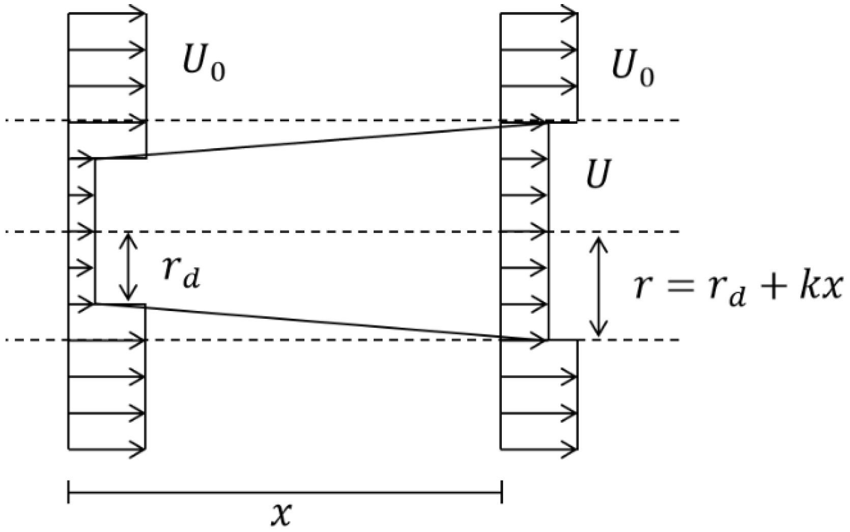
The Jensen wake model is widely used in wind farm layout optimization studies to calculate wake effects [34]. Assuming that the mass is conserved in the wake and the model is a top-hat shape, the wind speed U downstream the turbine is as follows:
where U0 is the inflow wind speed, a is the axial induction factor, rd is the wake impact radius, and k is the entrainment constant calculated based on empirical data (see Figure 1).

Figure 1.
Schematic of the Jensen wake model.
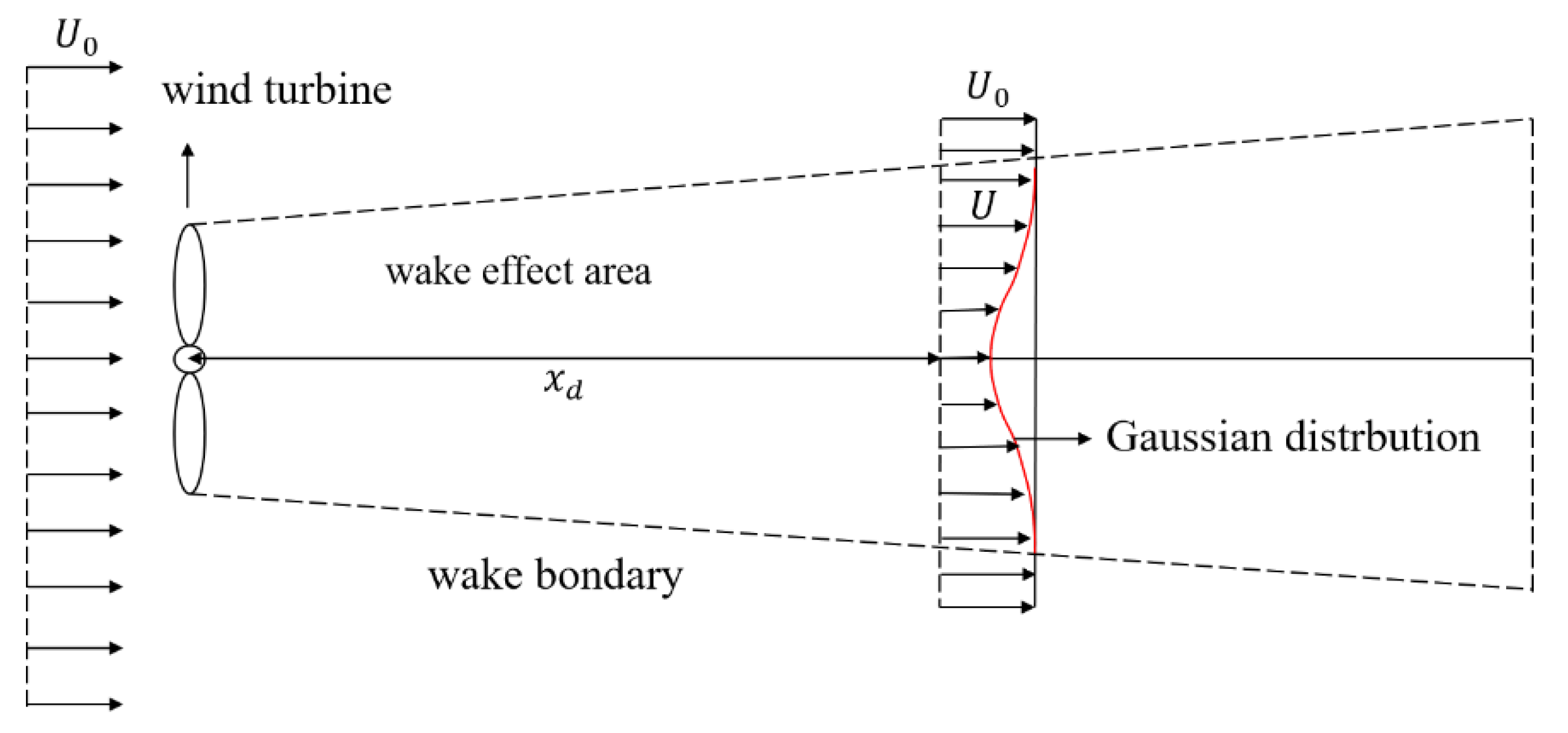
The Jensen wake model, which only considers mass conservation, tends to predict the velocity deficit at the center of the wake while overestimating it at the outer region of the wake. Then, Frandsen et al. [35] applied both mass and momentum conservation principles to a control volume around the turbine and proposed a revised expression for the wake velocity deficit. Nevertheless, the model still assumes a top-hat shape for the wake. Bastankhah et al. [36] pointed out that the Jensen wake model’s improper assessment of wind speed leads to significant errors in velocity predictions. They proposed an alternative wake deficit model following a Gaussian distribution. However, this model still presents challenges in terms of robustness and universality. To address the issue of the low wind speed prediction accuracy observed in the Jensen wake model, Ishihara et al. [37] proposed a wake cross-sectional velocity deficit model based on a Gaussian distribution, which is considered a more reasonable approach than the Jensen top-hat assumption. The velocity deficit in the Gaussian wake model is illustrated in Figure 2.

Figure 2.
Schematic of the Gaussian wake model (The red curve represents the Gaussian distribution).
The Gaussian wake model is derived from the assumptions of an axisymmetric and self-similar wake deficit. In comparison to the Jensen model, the Gaussian wake model can more accurately predict the wind speed deficit within the wake-affected region. Consequently, it exhibits a broader range of applicability. In the Gaussian wake model proposed by Ishihara et al. [37], the wind speed U at a specific location downstream with a downwind distance of xd and a crosswind distance of rd from the upstream turbine hub position is described as follows:
where F(CT, Ia, xd/D) represents the velocity deficit function at the downstream location xd along the downwind direction. ϕ(rd/σ) is the velocity deficit distribution function at the radial distance rd along the spanwise direction. CT refers to the thrust coefficient. Ia represents the ambient turbulence intensity. D is the rotor diameter of the wind turbine. σ is the typical wake width. h is the hub height. y is the horizontal distance from the specified point to the hub height, and z is the vertical distance from the specified point to the hub height.
The following parameters are obtained by fitting the experimental results and data [36]: , , , and .
To account for the impacts of multiple upstream wind turbine wakes on the downstream turbine, it is essential to calculate the effects of the wakes using wake superposition models. Commonly employed wake superposition models include the linear superposition model [38], the energy balance superposition model [39] and the sum of squares superposition model [40], which all are based on the cumulative flow characteristics within the superposition region formed by the wakes of all upstream turbines [41]. Among these models, the sum of squares superposition model assumes that the total kinetic energy deficit is equal to the sum of kinetic energy deficit from the upstream turbines. This model provides more accurate predictions compared to other models. Therefore, the sum of squares superposition model was selected for calculating the wind speed deficit of the downstream turbine.
When optimizing a wind farm layout using the Jensen wake model, the overlap area between the upstream wake and the rotor plane of the downstream turbine has an impact on average velocity of the rotor plane of downstream turbine. A uniform velocity distribution is assumed within the wake region to predict wind speed. The velocity of the i + 1 wind turbine behind multiple turbines is denoted as Ui+1 as follows:
where U0 represents the incoming wind speed, Ui represents the wake velocity affected only by the ith upstream turbine, n represents the number of turbines in the wind farm, and represents the overlap area between the wake of the ith upstream turbine and the rotor area Ar of the downstream turbine.
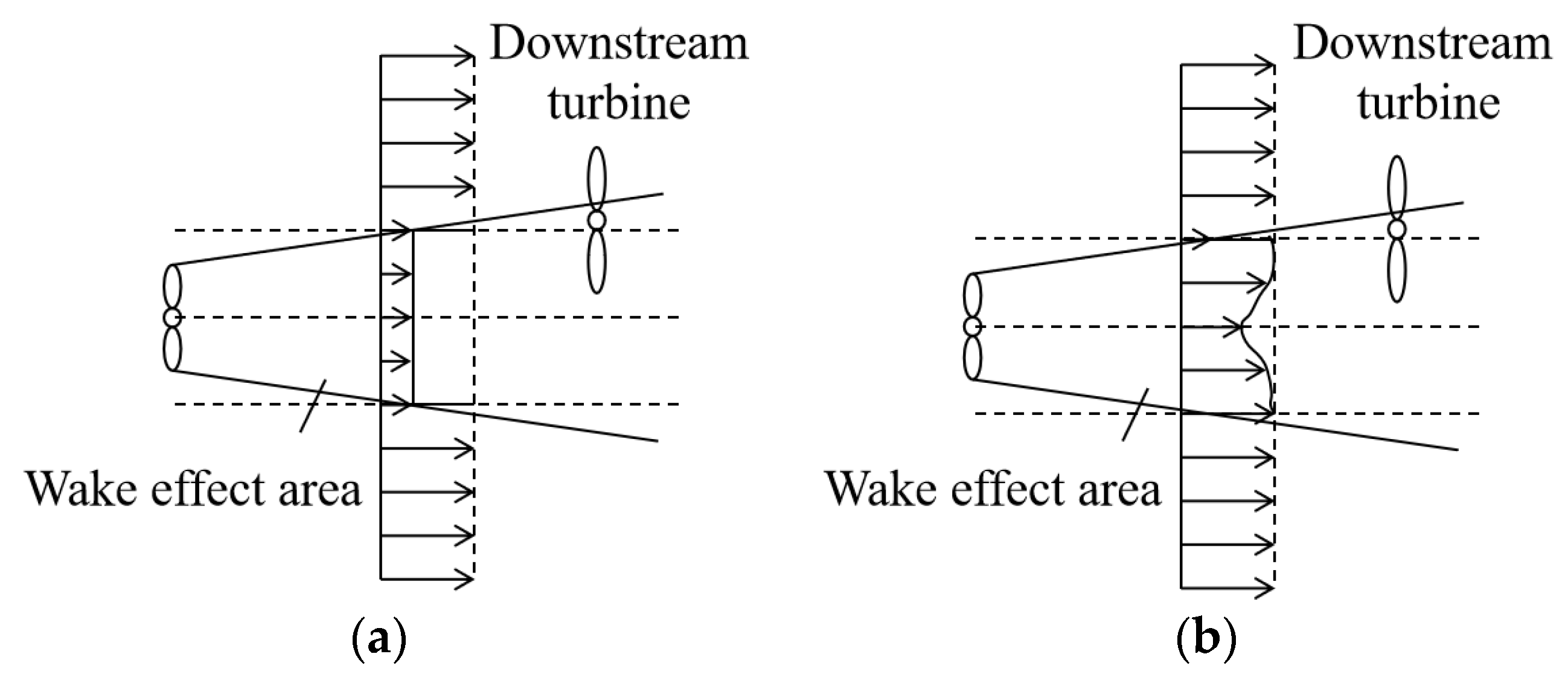
When optimizing the layout of a wind farm using the Gaussian wake model, the average wind speed of the entire rotor disk is calculated through the integration of wind speed within the disk. The Gaussian wake model provides a consistent description of the downstream wind speed, thereby obviating the necessity of an individual consideration of the overlapping region. The superposition diagram of the two wake models is illustrated in Figure 3. In wind farm optimization using the Gaussian wake model, the velocity of the i + 1 wind turbine denoted as Ui+1 after multiple turbines can be expressed as follows:

Figure 3.
Schematic diagram of wake superposition: (a) Jensen wake model and (b) Gaussian wake model.
2.2. Optimization Algorithm
2.2.1. Genetic Algorithm
Genetic algorithm is a famous meta-heuristic algorithm, inspired by the survival of the fittest theory proposed by Darwin in the process of biological evolution, and searches for the global optimal solution by imitating the principle of the survival of the fittest in nature. Genetic algorithm can evaluate multiple individuals and generate multiple optimal solutions, and so it has better global search ability than other optimization algorithms.
The genetic algorithm based on grid division in wind farm layout optimization research usually consists of the following steps:
- (1)
- Generate the initial population
The wind farm is divided into a certain number of grids, the fans are arbitrarily arranged in the center of the divided grid, and the layout is binary coded. One layout is an individual, randomly generating a certain number of individuals to form an initial population.
- (2)
- Chromosome fitness is calculated
The wind farm layout represented by individual decoding is substituted into the wake model and power function to calculate the fitness.
- (3)
- The roulette principle selects the next-generation population
The fitness of all individuals in the initial population is calculated, and the next-generation population is selected according to the genetic principle that the fitness of individuals is proportional to the probability.
- (4)
- Crossover operation to update the population
The crossover operation is performed with a certain probability: select two individuals in the new population, select any point, and exchange the chromosomes of the second half of the point of the two individuals. After the exchange, new individuals are placed in the new population.
- (5)
- Mutation operation to update the population
Perform a mutation operation with a certain probability: mutate the chromosome value of any point of an individual, that is, when the point is 0, it mutates to 1 in binary, and when it is 1, it mutates to 0. The mutant individuals are also placed in the new population.
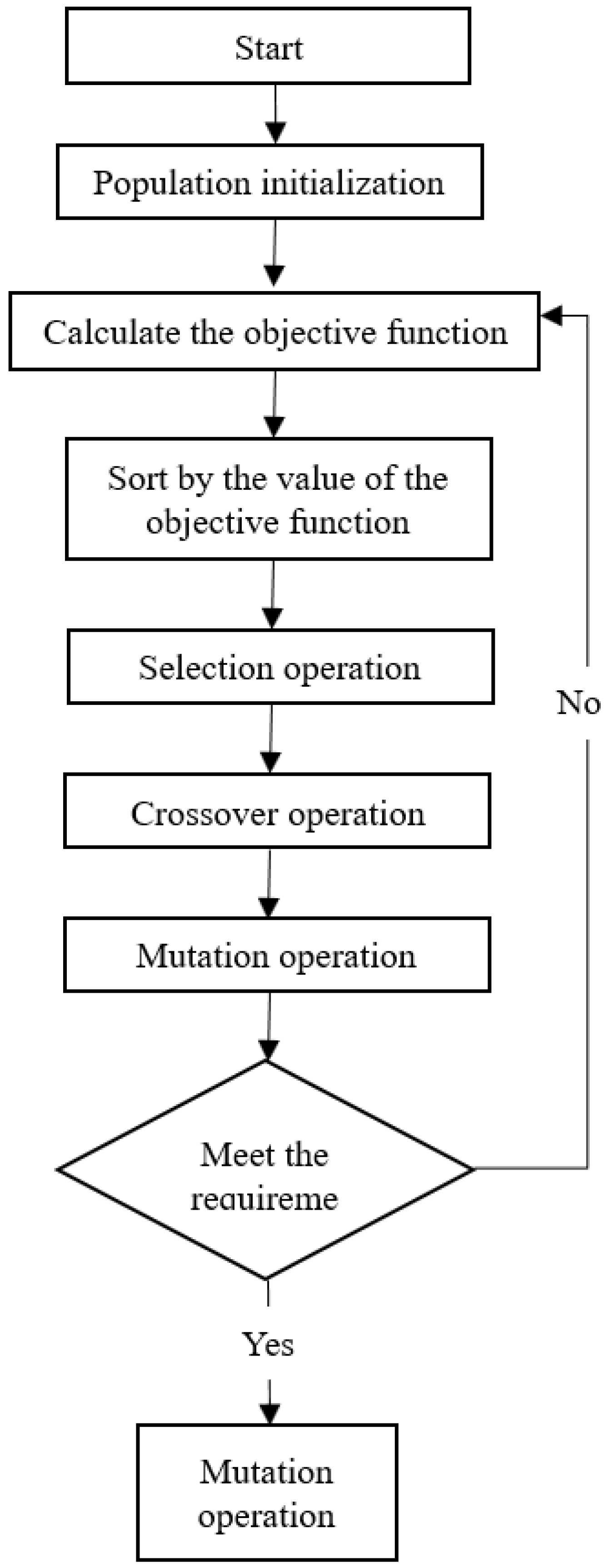
According to the above principles, the optimal wind farm layout can be obtained when the convergence condition is reached through the continuous iteration of the population. The optimization process is shown in Figure 4.

Figure 4.
The optimization process of the genetic algorithm.
This study employed a genetic algorithm (GA) for optimization. The number of individuals in the population was set to 300. The crossover rate was 0.9, indicating that 90% of the population produced offspring through crossover. The mutation rate was set to 0.1. The algorithm was run for 3000 generations to ensure convergence to a near-optimal solution. The optimization is conducted in a MATLAB text-based environment using a novel coding approach compared to previous studies. Matrix binary chromosomes were selected instead of numerical binary chromosomes, which significantly reduced the computation time and improved optimization results. In this study, the available terrain was divided into cells where turbines can be installed. The chromosomes are represented as 10 by 10 matrices, where ‘1’ indicates the presence of a turbine in the corresponding cell, and ‘0’ indicates the absence of a turbine. This representation simplifies the visualization and analysis of the wind farm layout.
2.2.2. Grid–Coordinate Two-Step Genetic Algorithm
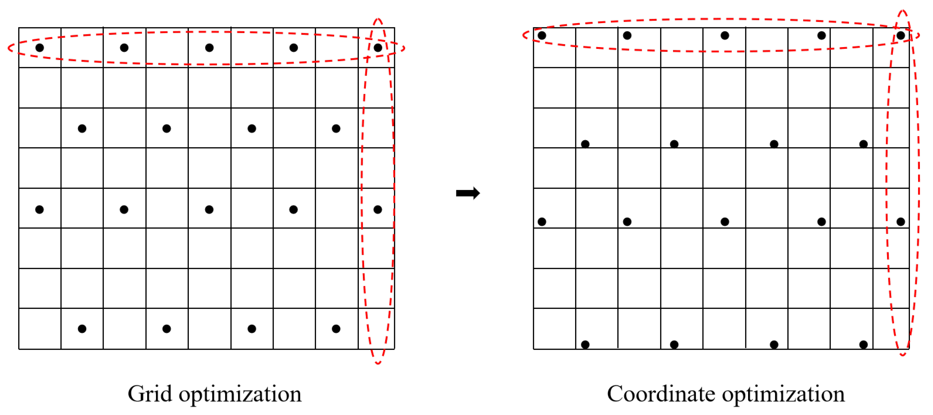
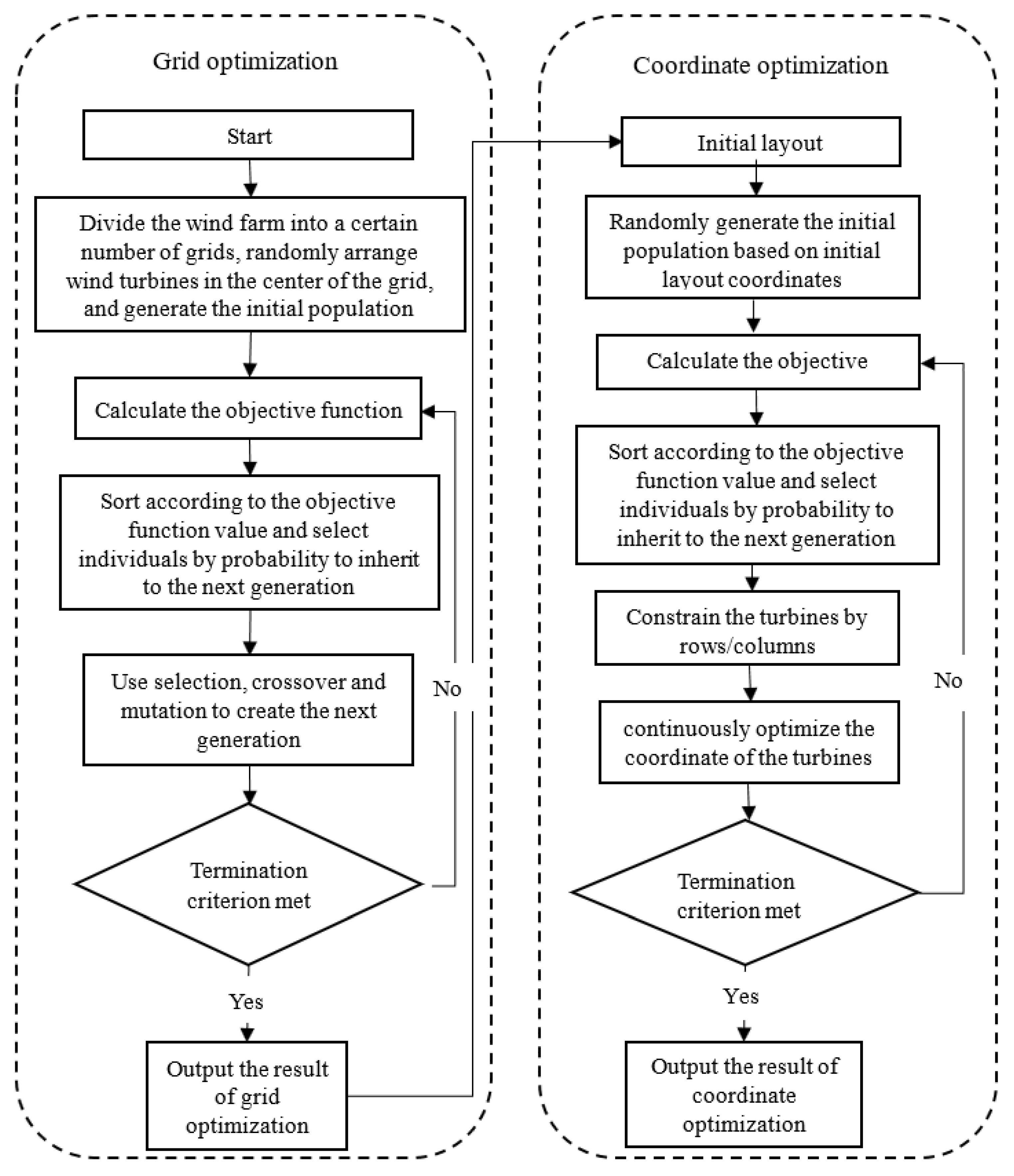
The optimization algorithm proposed in this paper consists of two steps, as shown in Figure 5. The first step is discrete optimization based on the grid-based genetic algorithm, which aims to determine the optimal number of wind turbines to maximize the power generation per unit cost. The grid-based genetic algorithm is employed to search for the best configuration within the given wind farm area. The second step focuses on continuous optimization using a coordinate-based genetic algorithm to build upon the grid-based initial layout, where the positions of wind turbines at the rows and columns are fine-tuned. The positions of wind turbines with respect to rows and columns are adjusted using the coordinate-based genetic algorithm to further improve the beauty of wind farm layout optimization. When a wind turbine is moved based on rows, the x-coordinate remains unchanged while the y-coordinate increases or decreases simultaneously. Conversely, when a wind turbine is moved based on columns, the y-coordinate remains unchanged while the x-coordinate changes.

Figure 5.
Schematic of wind turbine position adjustment (The black dots represent the location of the wind turbine, and the red curves frame the different results of the grid method and the coordinate method).
In this study, the objective function is the unit cost of power generation. Additionally, the detailed optimization process is illustrated in Figure 6. In the grid-based phase, discrete optimization of turbine locations is conducted to obtain the optimal number of turbines and the initial layout positioned at the center of each grid. Based on the initial grid layout, further optimization of turbine positions is carried out at the row/column level to achieve a more regular arrangement of the wind farm.
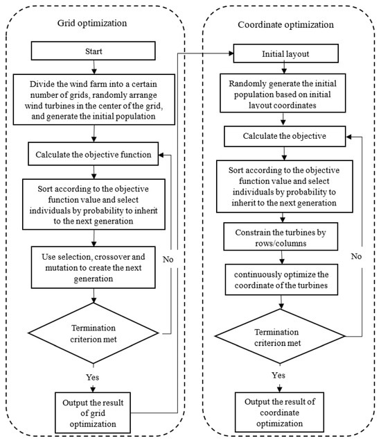
Figure 6.
Schematic diagram of the two-step algorithm.
2.2.3. Objective Function
The optimization procedure is based on the following objective function [21]:
Additionally, the construction cost of the wind farm was proposed by Mosetti [9] as follows:
where is the total power extracted by all of the N turbines in the wind farm, and is the number of turbines installed.
The total power P of wind farms can be simplified as follows [21]:
where is the incoming wind speed for the ith wind turbine.
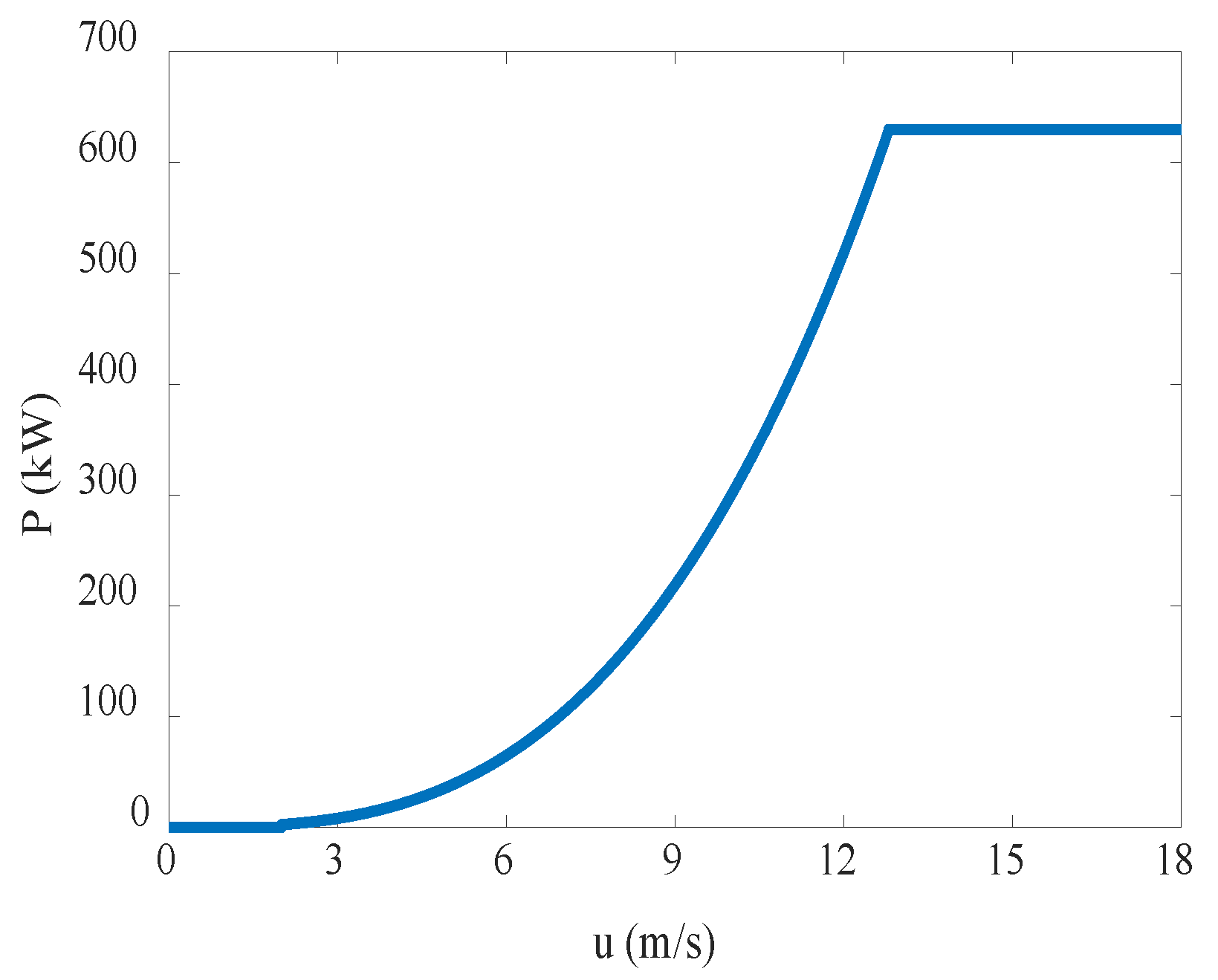
Equation (11) represents a simplified power generation formula for wind farms. However, it is important to note that in reality, the power output does not increase linearly with the cube of the wind speed beyond the rated wind speed. Additionally, wind turbines cease power generation beyond the cut-out wind speed. For wind conditions 1 and 2 (details provided in Section 3.1), where the wind speed is set at 12 m/s, the simplified power formula can be used since it is below the rated wind speed. However, in the case of wind condition 3, where the wind speed exceeds the rated wind speed, the simplified formula is not applicable. Instead, the power generation of the wind turbine is calculated using Equation (12), which takes into account the power curve of the wind turbine, as illustrated in Figure 7.
where the unit of P is kW.

Figure 7.
Power curve of a wind turbine.
The proportion of wake velocity deficit in a wind farm can be expressed by the efficiency of the wind farm as follows:
where P0 is the total power of wind farm operation without the wake influence.
3. Results and Discussion
An example analysis was conducted for a wind farm under four classical wind conditions and an actual wind condition. The primary objective of this optimization was to maximize the power generation per unit cost by obtaining an initial grid layout. Subsequently, the wind turbine coordinates were adjusted on a row–column basis to enhance the overall power generation of the wind farm. The wind turbine units and wind farm information used in the analysis are summarized in Table 1.

Table 1.
Information on the wind turbines and wind farm.
3.1. Case of a Classical Wind Field
The wind speed and wind direction of each classical wind condition are detailed as follows:
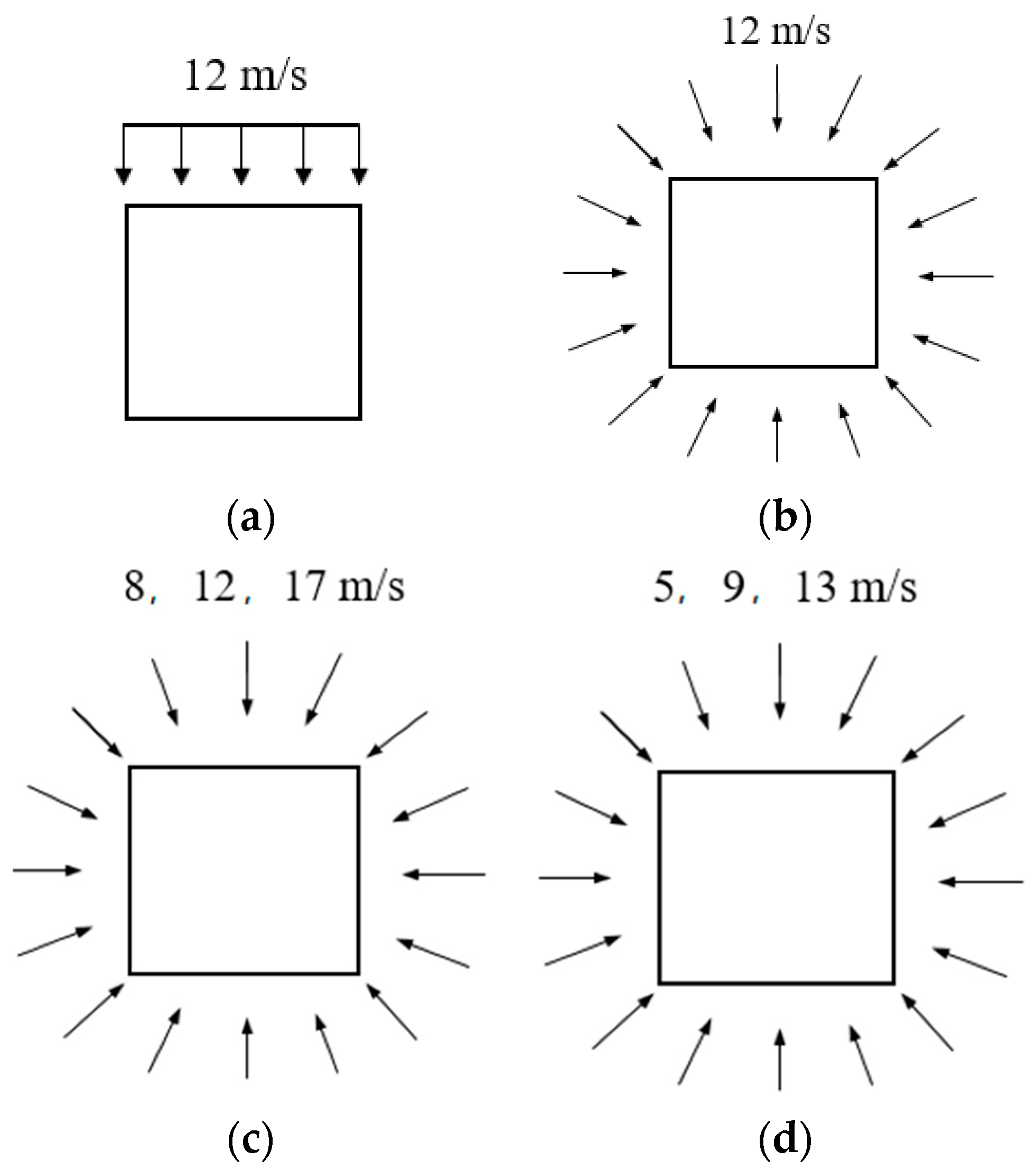
Case 1—single-wind-direction and constant wind speed condition where the wind speed is fixed at 12 m/s;
Case 2—multiple wind directions and constant wind speed condition, this scenario encompasses 36 wind directions, each with an equal probability (in 10° increments), and a constant wind speed of 12 m/s;
Case 3—multiple wind directions and variable wind speed condition, for this condition, there are also 36 wind directions (in 10° increments) with wind speeds of 8 m/s, 12 m/s, and 17 m/s.
To address the limitation of classical multiple wind directions and variable wind speed condition, where the high wind speed setting results in an average wind speed of 14 m/s that deviates from the actual wind farm conditions, an improvement was introduced to create a fourth scenario.
Case 4—Modified multiple wind directions and variable wind speed condition, this scenario comprises 36 wind directions (in 10° increments) with wind speeds of 5 m/s, 9 m/s, and 13 m/s. The illustrations for each wind condition can be found in Figure 8, and the probability distribution of wind direction and wind speed is shown in Figure 9. In cases 3 and 4, finding the optimal solution intuitively is challenging because the wind speed, direction, and frequency significantly influence the interactions between different turbines. For the wind distribution, as summarized in Figure 9, three wind intensities and 36 directions (at 10° intervals) are assumed. The frequency is represented as a fraction of the time unit during which a specific wind condition occurs.

Figure 8.
Wind scenarios: (a) unidirectional uniform wind (case 1); (b) uniform wind with variable directions (case 2); (c) non-uniform wind with variable directions (case 3); and (d) modified non-uniform wind with variable directions (case 4).
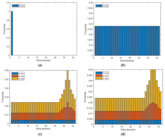
Figure 9.
Wind speed distributions under different directions: (a) unidirectional uniform wind; (b) uniform wind with variable directions; (c) non-uniform wind with variable directions; and (d) modified non-uniform wind with variable directions.
The wind farm layout optimization is performed using both the Jensen wake model and the Gaussian wake model. This optimization process follows a two-step approach. First, the grid-based optimization is used to establish the initial layout, considering power generation per unit cost. Once the number of wind turbines is determined, a subsequent coordinate-based re-optimization is performed, enhancing power generation by adjusting the positions of wind turbines in rows and columns. In the case of complex wind conditions characterized by multiple wind directions, a Cartesian coordinate transformation is essential for adapting the wind turbine coordinates, as recommended by Parada et al. [42]. This transformation enables the optimization process to account for the variability in wind directions and to precisely adjust the positions of wind turbines accordingly.
3.1.1. Unidirectional Uniform Wind
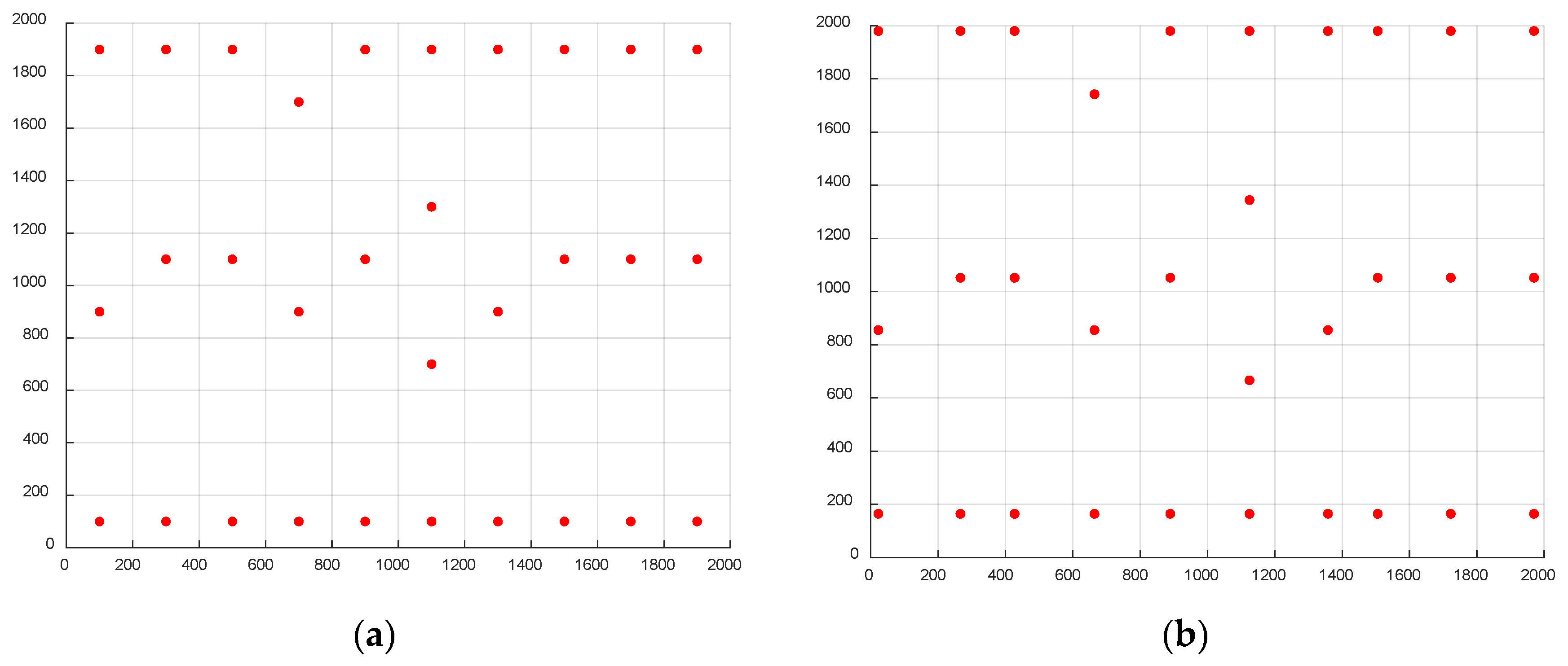
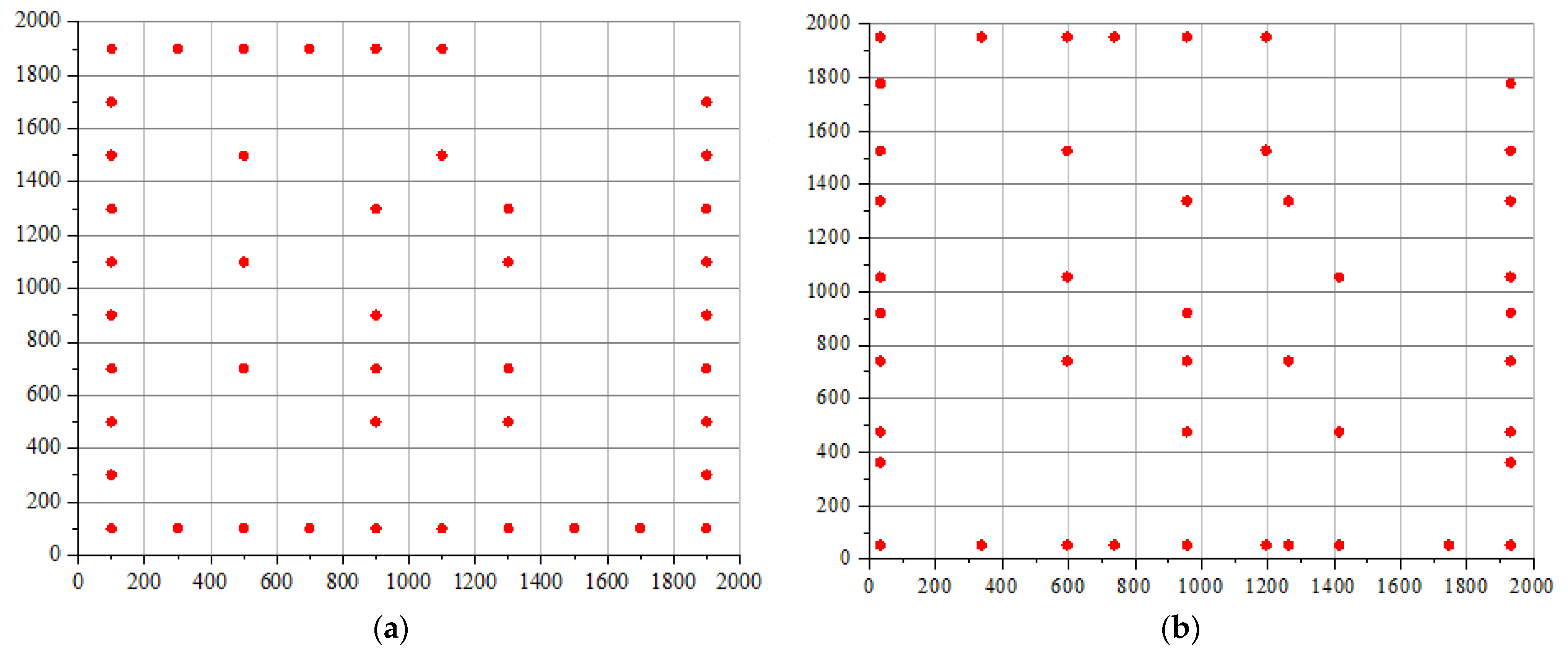
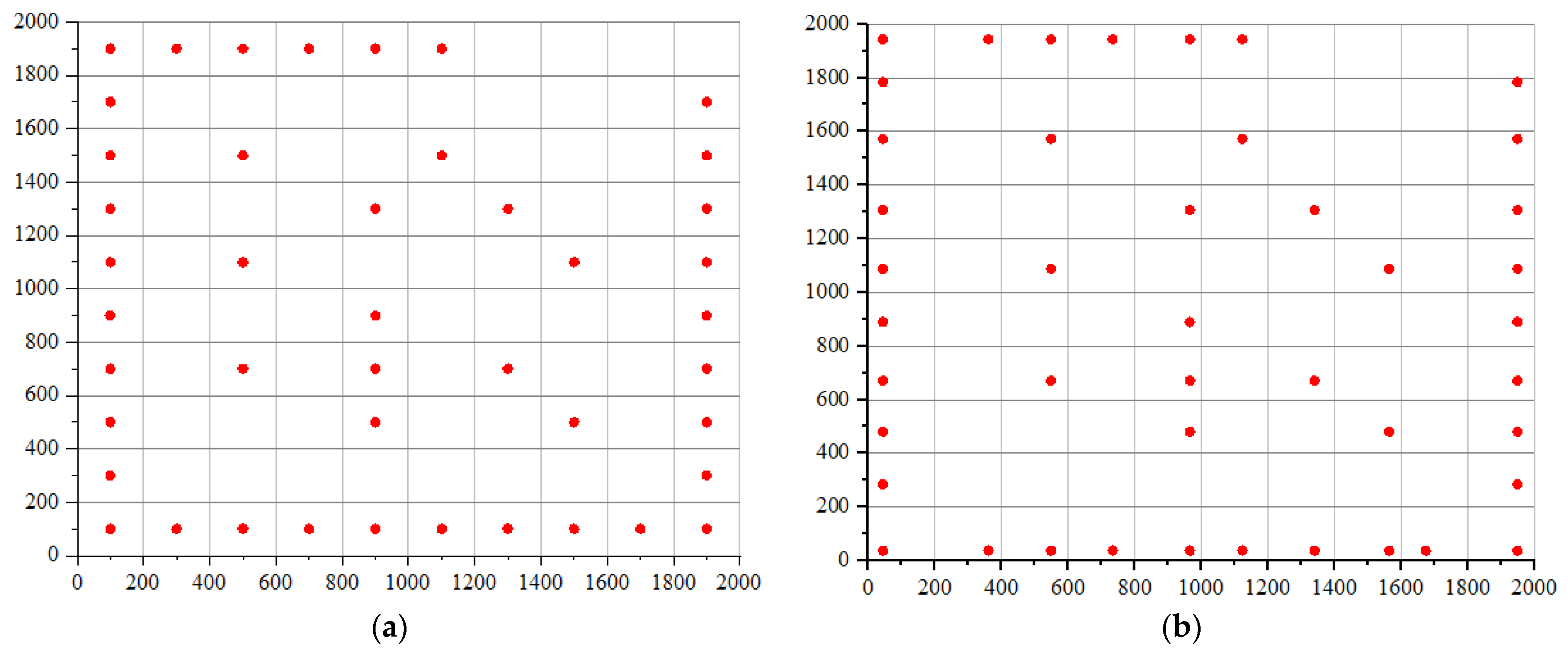
The optimization process begins with the grid-based algorithm to determine the optimal number of wind turbines for the single wind direction and constant wind speed scenario. Then, the coordinate-based method is employed to adjust the layout, with the overarching goal of maximizing the power generation within the wind farm. The optimized layouts using the Jensen wake model and the Gaussian wake model are shown in Figure 10 and Figure 11, respectively. A comprehensive summary of the layout optimization using both wake models can be found in Table 2.

Figure 10.
Optimal configuration of case 1 based on the Jensen wake model. (a) Grid optimization; (b) coordinate optimization (the red dot represents the location of the wind turbine, and in the figures below, the red dot is also assumed to be the location of the wind turbine by default).

Figure 11.
Optimal configuration of case 1 based on the Gaussian wake model. (a) Grid optimization; (b) coordinate optimization.

Table 2.
Optimization results for case 1: unidirectional uniform wind.
From Figure 11, it can be observed that following the coordinate-based optimization, the wind turbines located at the outer edge of the wind farm tend to move closer to the boundaries in both rows and columns. In contrast, turbines situated in the central area exhibit minor displacements and incline towards the prevailing wind direction. This phenomenon can be explained from the perspective of wake effects. Intuitively, the domain under consideration in this study employs a wake model where the wake diameter increases solely as a function of downstream distance. Consequently, a straightforward optimization of a single 10-cell column within the computational domain can be extrapolated to the entire domain to identify the optimal solution for this simplified wind scenario. The displacement towards the boundaries is conducive to more efficient land resource utilization within the wind farm, resulting in increased spacing between turbines. The turbines positioned in the central rows move away from the first row and closer to the last row, a strategic shift that aims to enhance power generation. Although this displacement trend increases the wake effects on the middle turbines, it subsequently reduces the wake effects on the turbines in the last row. As a consequence, the overall power generation of the wind farm experiences an increment.
Table 3 presents a comparison of the power output efficiency, total power, cost, power generation per unit cost, and the number of turbines for each configuration. Compared to the studies by Mosetti [9] and Grady [26], the increased number of turbines in the optimal configuration obtained in this study result in higher total power output for the wind farm. However, despite the increase in the number of turbines compared to Emami [28], which results in a decrease in the overall efficiency of the wind farm, with power generation efficiency dropping from approximately 100% to 93% and 91.99%, respectively, when considering costs, it is found that the unit cost of electricity generation from the optimization results of this study is the highest.

Table 3.
Comparison of solution characteristics—case 1, (i) Mosetti, (ii) Grady, (iii) Emami, and (iv) the present study.
3.1.2. Uniform Wind with Variable Directions
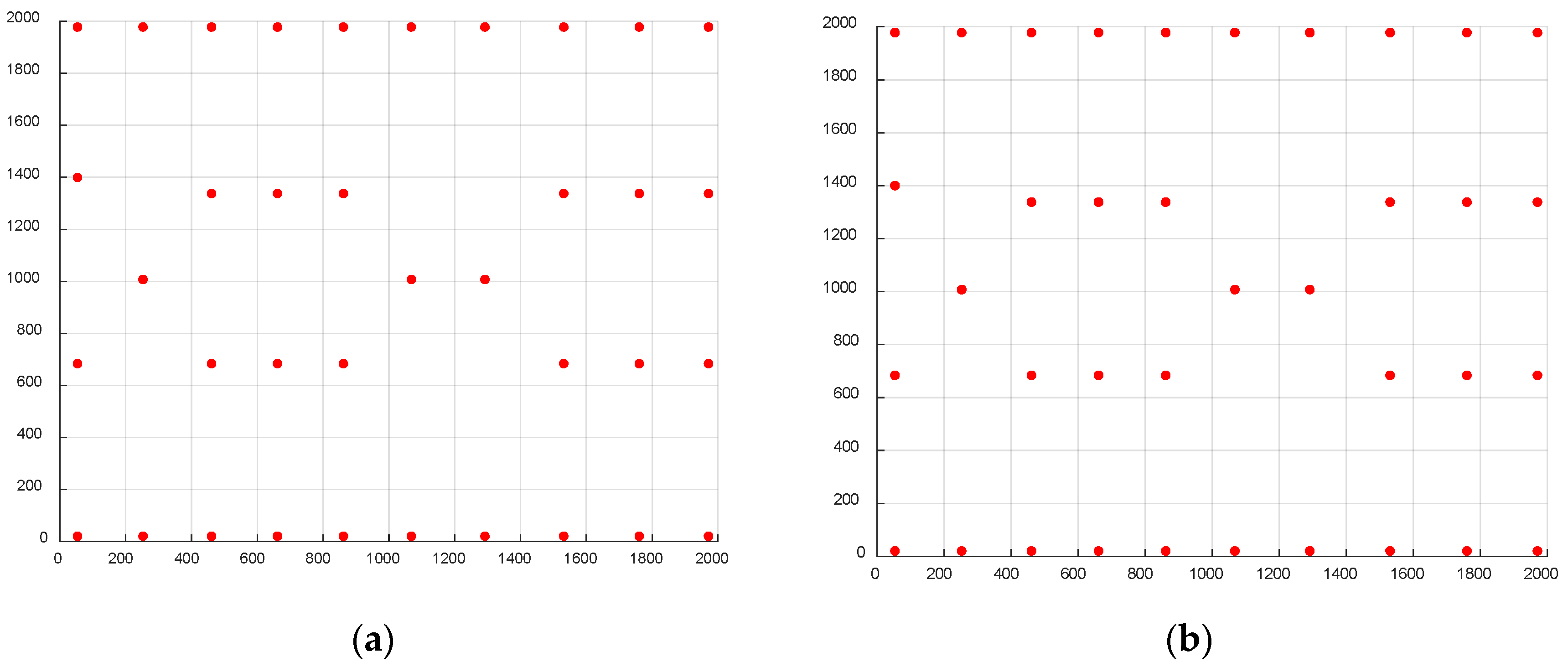
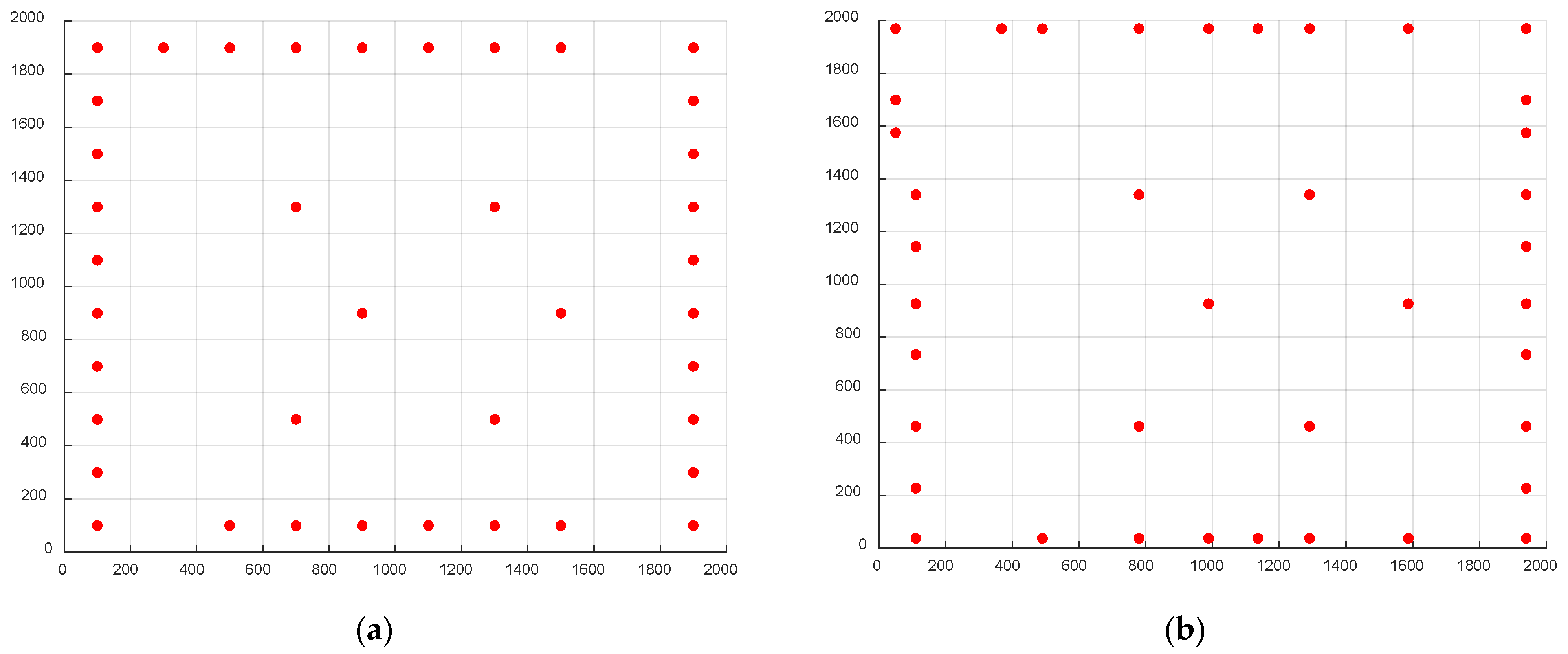
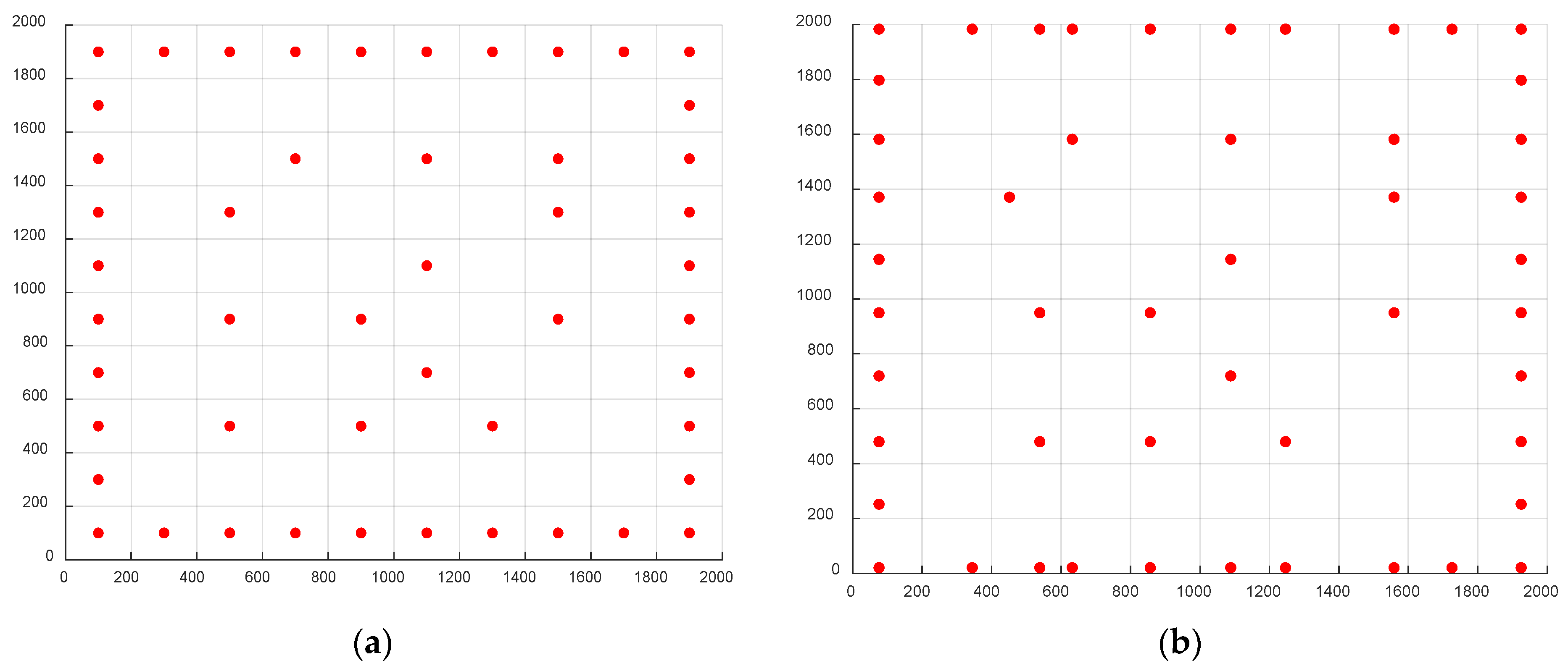
In the case of multi-directional wind with a constant wind speed, a preferable orientation does not exist. The efficiency of each turbine is primarily determined by the distance from other turbines. Thus, in this case, the initial step involved the grid-based method, resulting in layouts with 41 and 46 wind turbines when utilizing the Jensen wake model and the Gaussian wake model, respectively. Then, a coordinate-based continuous optimization was performed while adhering to row/column constraints. The optimized layouts are presented in Figure 12 and Figure 13, with a comprehensive summary of the results available in Table 4. It is noteworthy that in the coordinate-based optimized layouts, the wind turbines situated along the periphery of the wind farm exhibit a tendency to spread toward the boundaries, consequently leading to increased spacing between the outer and inner turbines. In contrast, the displacements of the inner turbines are relatively smaller in magnitude.

Figure 12.
Optimal configuration of case 2 based on the Jensen wake model. (a) Grid optimization; (b) coordinate optimization.
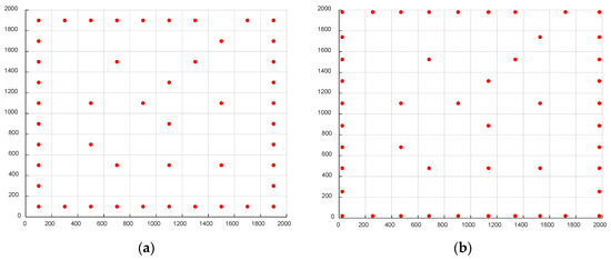
Figure 13.
Optimal configuration of case 2 based on the Gaussian wake model. (a) Grid optimization; (b) coordinate optimization.

Table 4.
Optimization results for case 2: uniform wind with variable directions.
Table 5 compares the optimal configurations from three classical studies [9,26,28] with the optimal configuration of this study. The results clearly indicate that the new configuration using the Gaussian wake model achieves higher total power output, electricity generation, and unit cost of electricity generation by employing more turbines. Additionally, even under the optimized configuration using the Jensen wake model, the unit cost of electricity generation is higher than the optimization results from the other three literature [9,26,28] sources.

Table 5.
Comparison of solution characteristics—case 2, (i) Mosetti, (ii) Grady, (iii) Emami, and (iv) the present study.
3.1.3. Non-Uniform Wind with Variable Directions
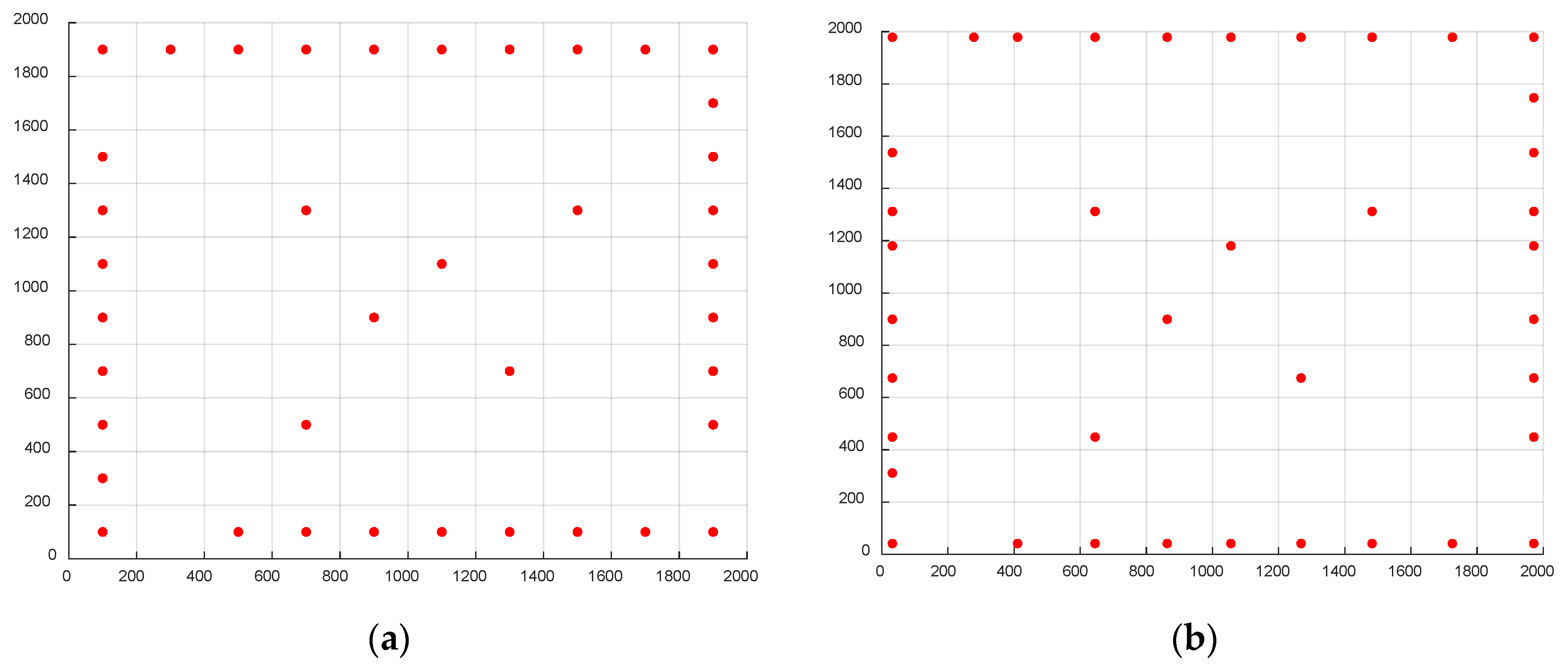
For the more complex case of multi-directional wind, the optimal solution cannot be determined empirically. However, it is assumed that a similarly ordered solution is achievable. In the example provided by Mosetti et al. [9], this resulted in a configuration where turbines were distributed around the outer perimeter of the domain, with few turbines placed in the center. Power generation of the turbine can be calculated using Equation (9) and substituted into the objective function. Wind farm layout optimization is performed for both the Jensen wake model and the Gaussian wake model under the multiple wind directions and variable wind speed scenario. The optimized layouts are shown in Figure 14 and Figure 15, with the corresponding results presented in Table 6. The results indicate that the outer wind turbines still exhibit a tendency to disperse outward, increasing the distance from the inner turbines. The efficiency of the two optimization methods improved by approximately 5.62% and 2.25%, respectively. Notably, optimization based on the Gaussian wake model outperformed that based on the Jensen wake model.
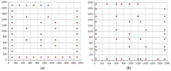
Figure 14.
Optimal configuration of case 3 based on the Jensen wake model. (a) Grid optimization; (b) coordinate optimization.
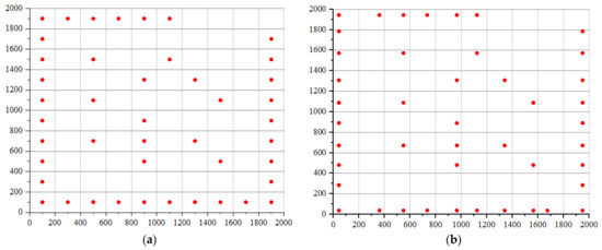
Figure 15.
Optimal configuration of case 3 based on the Gaussian wake model. (a) Grid optimization; (b) coordinate optimization.

Table 6.
Optimization results for case 3: non-uniform wind with variable directions.
Table 7 compares the optimal configurations from three seminal studies [9,26,28] with those obtained in this research. The results clearly demonstrate that under the new optimal configuration using the Gaussian wake model proposed in this paper, the efficiency achieved through the two-step optimization surpasses that reported in the other three studies. Additionally, the power generation per unit cost is highest under this configuration. Conversely, while the efficiency of the optimized results based on the Jensen wake model is lower than that reported in the literature [28], the unit power generation exceeds the values reported in the same literature.

Table 7.
Comparison of solution characteristics—case 3, (i) Mosetti, (ii) Grady, (iii) Emami, and (iv) the present study.
3.1.4. Modified Non-Uniform Wind with Variable Directions
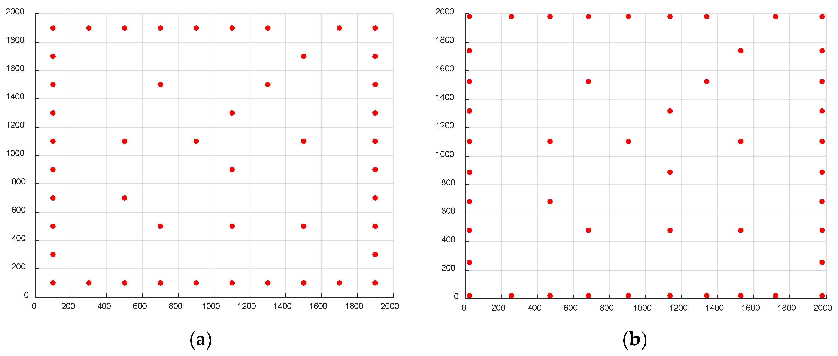
Similarly, the power generation of the turbine can be calculated using Equation (9), and wind farm layout optimization is performed based on both the Jensen wake model and the Gaussian wake model under the improved multiple wind directions and variable wind speed scenario. The optimized layouts are visually depicted in Figure 16 and Figure 17, and the results are presented in Table 8. Table 9 includes the values for the total power, efficiency, number of turbines, and cost for the modified non-uniform wind with variable directions case. Notably, it can be observed that the trend of outer wind turbines shifting towards the periphery of the wind farm persists, with a greater number of turbines positioned in wind directions characterized by a high wind speed probability. An analysis of the outcomes displayed in Table 5 reveals that the optimization based on the Jensen wake model achieved a 0.42% improvement, whereas the optimization based on the Gaussian wake model realized a more substantial 1.01% enhancement, surpassing the results of the Jensen wake model optimization. Furthermore, both optimized wind farms demonstrate higher efficiency compared to the classical multiple wind directions with variable wind speeds modified scenario.

Figure 16.
Optimal configuration of case 4 based on the Jensen wake model. (a) Grid optimization; (b) coordinate optimization.

Figure 17.
Optimal configuration of case 4 based on the Gaussian wake model. (a) Grid optimization; (b) coordinate optimization.

Table 8.
Optimization results for case 4: improved non-uniform wind with variable directions.

Table 9.
Results for case 4.
Upon comparing the optimization results presented above, it becomes evident that the Jensen wake model optimization yields a power improvement ranging from 0.42% to 3.5%, while the optimization based on the Gaussian wake model achieves a power improvement of approximately 0.80–1.50% under the four classical wind conditions and the actual wind farm case. Notably, in case 1 and case 2, the Jensen wake model calculations produce a substantial improvement compared to the Gaussian wake model calculations. When optimizing for the four wind conditions using the Gaussian wake model, the improvements in case 1 and case 2 are lower than those in case 3 and case 4. In summary, the power per unit cost calculated using the Jensen wake model for the same layout is lower than that calculated using the Gaussian wake model. Additionally, when considering the same wind condition, the optimal number of turbines calculated using the Gaussian wake model is higher than that obtained using the Jensen wake model.
Although the Jensen wake model optimization produces a higher percentage of improvement for cases 1 and 2 compared to the Gaussian wake model optimization, it is essential to recognize that the Jensen wake model tends to overestimate wake effects and velocity deficits. Consequently, the perceived greater optimization potential with the Jensen wake model can lead to falsely inflated power output improvements. Furthermore, when considering the power improvement for layouts obtained through Jensen wake model optimization in case 3 and case 4 calculated using the Gaussian wake model, the improvements are negligible. From the perspective of wind farm power efficiency, it becomes evident that optimization based on the Gaussian wake model significantly outperforms the Jensen wake model optimization. This observation underscores the Gaussian wake model’s capacity to provide more accurate predictions of velocity deficits, leading to superior optimization results. Ultimately, this enhanced accuracy enables a more effective utilization of wind energy resources.
3.2. Application in an Actual Wind Farm
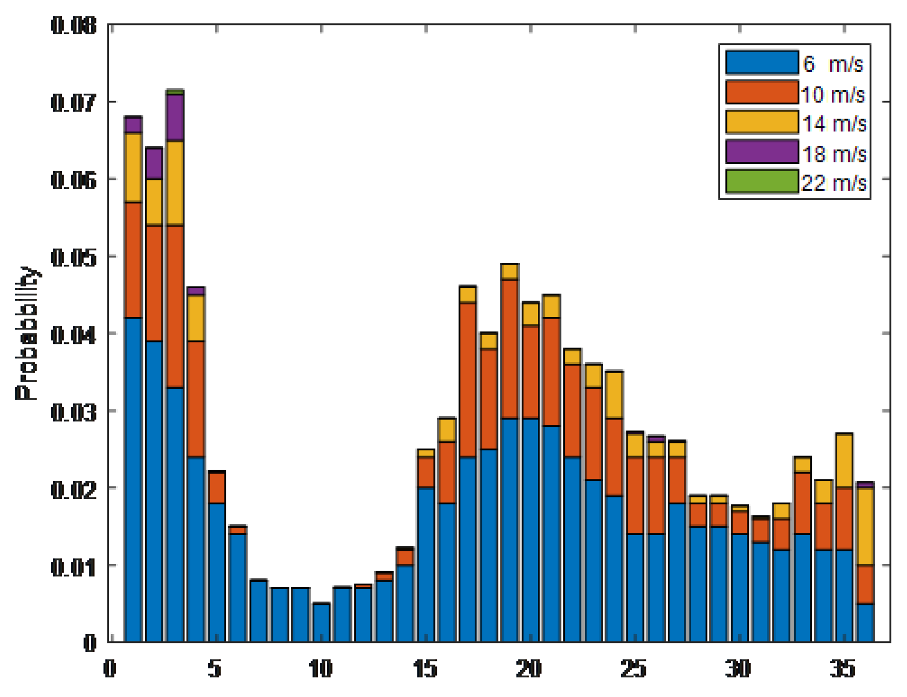
The analysis of classical wind field cases presented in Section 3.1 reveals that the proposed method not only fulfills the aesthetic requirements of wind farms but also effectively enhances power generation. Nevertheless, it is important to acknowledge that the adopted wind condition may not accurately represent real-world wind farm scenarios. Therefore, in the context of practical engineering applications, actual measured wind data are utilized as the inflow wind source. The average wind speed in this scenario measures 8.01 m/s, with the distribution of wind conditions and wind speed shown in Figure 18 and Figure 19.
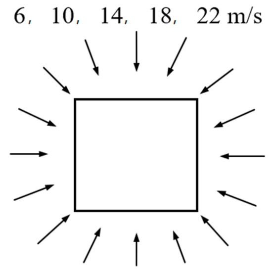
Figure 18.
Wind scenarios for a real case.

Figure 19.
Wind speed distribution across different directions for the real case.
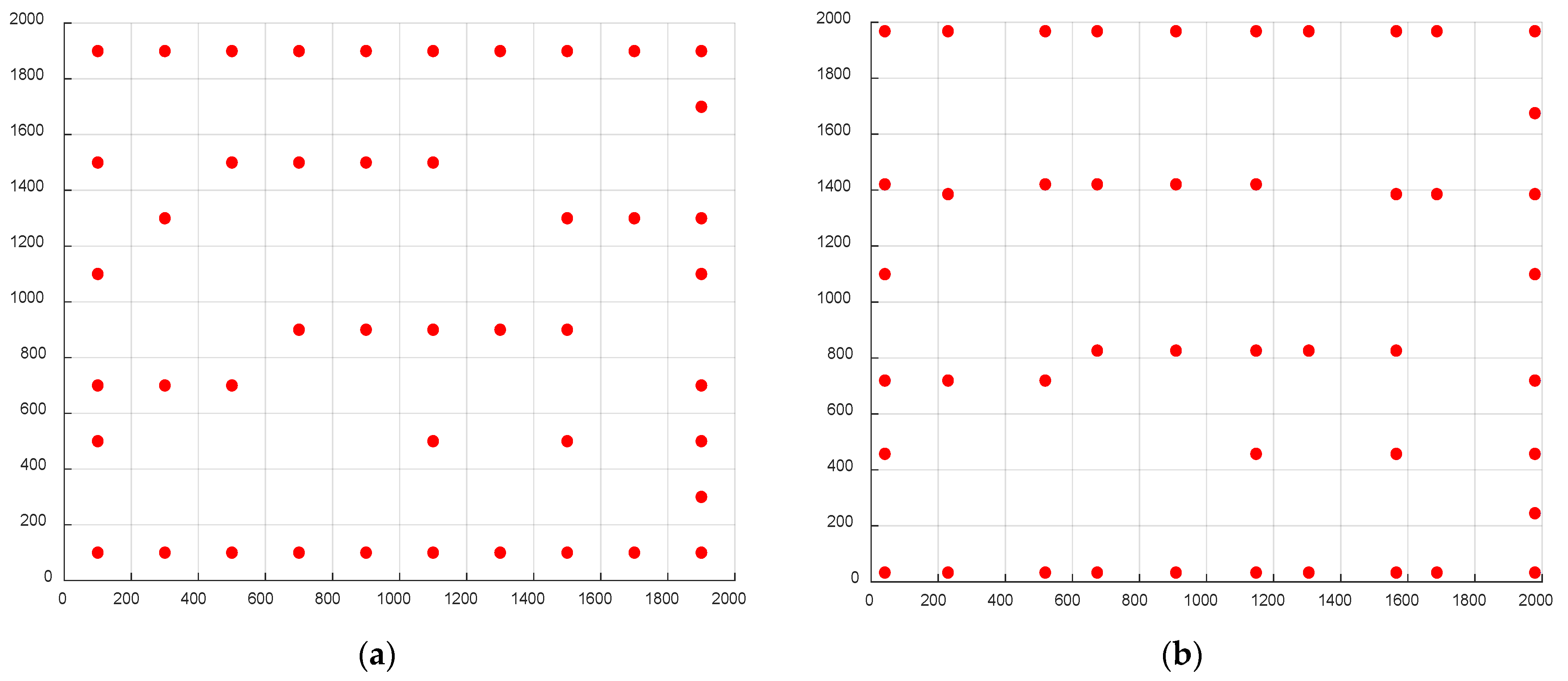
To ensure that wind turbines adhere to designated boundaries, a reserved distance of 0.5D is maintained around the boundaries, and the minimum spacing between each pair of turbines is set to 3D. In this case, the optimization process follows a similar approach to the previous scenario, with the only difference being the utilization of the Gaussian wake model for the optimized layout, as depicted in Figure 20. It is noteworthy that, akin to the previous case, the turbines on the outer periphery tend to spread towards the boundaries. The results of this optimization are presented in Table 10, indicating an approximate 1.00% increase in power generation for the wind farm. The improvement surpasses the optimization based on the Gaussian wake model in the previous classical wind condition case. Table 11 includes the values for the total power, efficiency, number of turbines, and cost for the actual wind farm case.

Figure 20.
Optimized layout based on the Gaussian wake model for the real case. (a) Grid optimization; (b) coordinate optimization.

Table 10.
Optimization results for the real case.

Table 11.
Results for the actual wind farm case.
4. Conclusions
This paper proposes a regular layout grid–coordinate two-step optimization method based on the Gaussian wake model. In the first step, a grid-based approach is employed to determine the optimal number and initial arrangement of wind turbines in the wind farm, aiming to minimize the cost of power generation. The second step is to move coordinates of the grid layout with row/column constraints while maintaining the regular layout to further improve the power generation of the wind farm. This method aims to maximize power generation while meeting the aesthetic requirements of wind farms. To validate the effectiveness of the proposed method, classical scenarios and actual wind farm cases are analyzed using both the Gaussian wake model and the Jensen wake model. The research observation findings can be summarized as follows:
(1) The analysis provided demonstrates that for classical conditions 1 and 2, the efficiency improvement of the two-step optimization method using the Gaussian wake model relative to the Jensen wake model is not significantly greater than that achieved by the initial grid optimization method. This is primarily because the Jensen model tends to overestimate the wake velocity deficit, thereby leaving less room for improvement. However, for conditions 3 and 4 (multiple wind directions, variable wind speed), the optimization effectiveness of the Gaussian wake model surpasses that of the Jensen wake model.
(2) When comparing the results of classic wind conditions with the optimization outcomes of Mosetti [9], Grady [26], and Emami [28], it is observed that for classic conditions 1 and 2, the efficiency of power generated in this study is comparable to that of three studies, yet the total power output and the unit cost of electricity generation are higher in this study. However, for classic condition 3, an increase in the number of wind turbines leads to greater wake effects and increased costs.
In real wind farms, actual terrain changes significantly influence turbine placement. The optimal layout method proposed in this paper is based on research conducted on flat terrain. Additionally, the service life of wind turbines is directly related to the overall economic benefits of wind farms, making fatigue optimization crucial for layout optimization. Addressing this aspect will be the subject of future research.
Author Contributions
Conceptualization, G.H. and K.L.; formal analysis and writing—original draft preparation, K.L. and Y.C.; methodology and validation, S.Z.; investigation, J.L.; resources, M.L. All authors have read and agreed to the published version of the manuscript.
Funding
This research was funded by Chongqing Technical Innovation and Application Development Research (CSTB2022TLADKPX0046), the Chongqing Technology Innovation and Application Development Project (cstc2021jscx-jbgsX0003), the 111 Project (B18062), Science and Technology R & D Project of Shandong Province (2022TSGC2024), and Jinan Innovation Team Project (2020GXRC045), which are greatly acknowledged.
Data Availability Statement
The original contributions presented in the study are included in the article, further inquiries can be directed to the corresponding author.
Acknowledgments
This work was supported by Chongqing Technical Innovation and Application Development Research, the Chongqing Technology Innovation and Application Development Project, the 111 Project, Science and Technology R & D Project of Shandong Province, and Jinan Innovation Team Project, which are greatly acknowledged.
Conflicts of Interest
Author Jiangke Luo was employed by the company PowerChina Chongqing Engineering Corporation Limited. The remaining authors declare that the research was conducted in the absence of any commercial or financial relationships that could be construed as a potential conflict of interest.
References
- Cheng, X.; Yan, B.; Zhou, X.; Yang, Q.; Huang, G.; Su, Y.; Yang, W.; Jiang, Y. Wind resource assessment at mountainous wind farm: Fusion of RANS and vertical multi-point on-site measured wind field data. Appl. Energy 2024, 363, 123116. [Google Scholar] [CrossRef]
- Perez-Moreno, S.S.; Zaaijer, M.B.; Bottasso, C.L.; Dykes, K.; Merz, K.O.; Réthoré, P.; Zahle, F. National Renewable Energy Laboratory NREL Golden CO US. Roadmap to the multidisciplinary design analysis and optimisation of wind energy systems. J. Phys. Conf. Ser. 2016, 753, 62011. [Google Scholar] [CrossRef]
- Perez-Moreno, S.S.; Dykes, K.; Merz, K.O.; Zaaijer, M.B.; National Renewable Energy Laboratory NREL Golden CO US. Multidisciplinary design analysis and optimisation of a reference offshore wind plant. J. Phys. Conf. Ser. 2018, 1037, 42004. [Google Scholar] [CrossRef]
- Mittal, P.; Kulkarni, K.; Mitra, K. A Novel and Efficient Hybrid Optimization Approach for Wind Farm Micro-siting. Ifac-PapersOnLine 2015, 48, 397–402. [Google Scholar] [CrossRef][Green Version]
- Mittal, P.; Kulkarni, K.; Mitra, K. A novel hybrid optimization methodology to optimize the total number and placement of wind turbines. Renew. Energy 2016, 86, 133–147. [Google Scholar] [CrossRef]
- Brogna, R.; Feng, J.; Sørensen, J.N.; Shen, W.Z.; Porté-Agel, F. A new wake model and comparison of eight algorithms for layout optimization of wind farms in complex terrain. Appl. Energy 2020, 259, 114189. [Google Scholar] [CrossRef]
- Liang, Z.; Liu, H. Layout Optimization of a Modular Floating Wind Farm Based on the Full-Field Wake Model. Energies 2022, 15, 809. [Google Scholar] [CrossRef]
- Gao, X.; Yang, H.; Lu, L. Optimization of wind turbine layout position in a wind farm using a newly-developed two-dimensional wake model. Appl. Energy 2016, 174, 192–200. [Google Scholar] [CrossRef]
- Mosetti, G.P.C.D.B.; Poloni, C.; Diviacco, B. Optimization of wind turbine positioning in large windfarms by means of a genetic algorithm. J. Wind Eng. Ind. Aerodyn. 1994, 51, 105–116. [Google Scholar] [CrossRef]
- Marmidis, G.; Lazarou, S.; Pyrgioti, E. Optimal placement of wind turbines in a wind park using Monte Carlo simulation. Renew. Energy 2008, 33, 1455–1460. [Google Scholar] [CrossRef]
- Bilbao, M.; Alba, E. Simulated annealing for optimization of wind farm annual profit. In Proceedings of the IEEE 2009 2nd International Symposium on Logistics and Industrial Informatics, Linz, Austria, 10–12 September 2009; pp. 1–5. [Google Scholar]
- González, J.S.; Rodriguez, A.G.G.; Mora, J.C.; Santos, J.R.; Payan, M.B. Optimization of wind farm turbines layout using an evolutive algorithm. Renew. Energy 2010, 35, 1671–1681. [Google Scholar] [CrossRef]
- Şişbot, S.; Turgut, Ö.; Tunç, M.; Çamdalı, Ü. Optimal positioning of wind turbines on Gökçeada using multi-objective genetic algorithm. Wind Energy Int. J. Prog. Appl. Wind Power Convers. Technol. 2010, 13, 297–306. [Google Scholar] [CrossRef]
- Feng, J.; Shen, W.Z.; Xu, C. Multi-objective random search algorithm for simultaneously optimizing wind farm layout and number of turbines. J. Phys. Conf. Ser. 2016, 753, 032011. [Google Scholar] [CrossRef]
- Biswas, P.P.; Suganthan, P.N.; Amaratunga, G.A. Decomposition based multi-objective evolutionary algorithm for windfarm layout optimization. Renew. Energy 2018, 115, 326–337. [Google Scholar] [CrossRef]
- Ituarte-Villarreal, C.M.; Espiritu, J.F. Optimization of wind turbine placement using a viral based optimization algorithm. Complex. Adapt. Syst. 2011, 6, 469–474. [Google Scholar] [CrossRef]
- Chowdhury, S.; Zhang, J.; Messac, A.; Castillo, L. Unrestricted wind farm layout optimization (UWFLO): Investigating key factors influencing the maximum power generation. Renew. Energy 2012, 38, 16–30. [Google Scholar] [CrossRef]
- Eroğlu, Y.; Seçkiner, S.U. Design of wind farm layout using ant colony algorithm. Renew. Energy 2012, 44, 53–62. [Google Scholar] [CrossRef]
- Turner, S.D.O.; Romero, D.A.; Zhang, P.Y.; Amon, C.H.; Chan, T.C.Y. A new mathematical programming approach to optimize wind farm layouts. Renew. Energy 2014, 63, 674–680. [Google Scholar] [CrossRef]
- Padron, A.S.; Stanley, A.P.J.; Thomas, J.J.; Alonso, J.J.; Ning, A. Polynomial chaos for the computation of annual energy production in wind farm layout optimization. J. Phys. Conf. Ser. 2016, 753, 032021. [Google Scholar] [CrossRef]
- Shakoor, R.; Hassan, M.Y.; Raheem, A.; Rasheed, N. Wind farm layout optimization using area dimensions and definite point selection techniques. Renew. Energy 2016, 88, 154–163. [Google Scholar] [CrossRef]
- Gualtieri, G. Comparative analysis and improvement of grid-based wind farm layout optimization. Energy Convers. Manag. 2020, 208, 112593. [Google Scholar] [CrossRef]
- Dykes, K. Optimization of Wind Farm Design for Objectives Beyond LCOE. J. Phys. Conf. Ser. 2020, 1618, 42039. [Google Scholar] [CrossRef]
- Stanley, A.P.J.; Ning, A. Massive simplification of the wind farm layout optimization problem. Wind Energy Sci. 2019, 4, 663–676. [Google Scholar] [CrossRef]
- Thomas, J.J.; Baker, N.F.; Malisani, P.; Quaeghebeur, E.; Sanchez Perez-Moreno, S.; Jasa, J.; Bay, C.; Tilli, F.; Bieniek, D.; Robinson, N.; et al. A comparison of eight optimization methods applied to a wind farm layout optimization problem. Wind Energy Sci. 2023, 8, 865–891. [Google Scholar] [CrossRef]
- Grady, S.A.; Hussaini, M.Y.; Abdullah, M.M. Placement of wind turbines using genetic algorithms. Renew. Energy 2005, 30, 259–270. [Google Scholar] [CrossRef]
- Wan, C.; Wang, J.; Yang, G.; Zhang, X. Optimal siting of wind turbines using real-coded genetic algorithms. In Proceedings of the European Wind Energy Association Conference and Exhibition, Marseille, France, 16–19 March 2009; pp. 1–6. [Google Scholar]
- Emami, A.; Noghreh, P. New approach on optimization in placement of wind turbines within wind farm by genetic algorithms. Renew. Energy 2010, 35, 1559–1564. [Google Scholar] [CrossRef]
- Geem, Z.W.; Hong, J. Improved Formulation for the Optimization of Wind Turbine Placement in a Wind Farm. Math. Probl. Eng. 2013, 2013, 481364. [Google Scholar] [CrossRef]
- Pillai, A.C.; Chick, J.; Khorasanchi, M.; Barbouchi, S.; Johanning, L. Application of an offshore wind farm layout optimization methodology at Middelgrunden wind farm. Ocean. Eng. 2017, 139, 287–297. [Google Scholar] [CrossRef]
- Yang, Q.; Hu, J.; Law, S. Optimization of wind farm layout with modified genetic algorithm based on boolean code. J. Wind Eng. Ind. Aerodyn. 2018, 181, 61–68. [Google Scholar] [CrossRef]
- Jiang, Q.; Zheng, H.; Yang, Q.; Zhou, X.; Huang, G.; Lin, Y. Wind farm layout optimization based on grid-coordinate genetic algorithm. Acta Sol. Energy Sin. 2022, 43, 266. [Google Scholar]
- Masoudi, S.M.; Baneshi, M. Layout optimization of a wind farm considering grids of various resolutions, wake effect, and realistic wind speed and wind direction data: A techno-economic assessment. Energy 2022, 244, 123188. [Google Scholar] [CrossRef]
- Jensen, N.O. A Note on Wind Generator Interaction; Risø National Laboratory: Roskilde, Denmark, 1983. [Google Scholar]
- Frandsen, S.; Barthelmie, R.; Pryor, S.; Rathmann, O.; Larsen, S.; Højstrup, J.; Thøgersen, M. Analytical modelling of wind speed deficit in large offshore wind farms. Wind Energy Int. J. Prog. Appl. Wind Power Convers. Technol. 2006, 9, 39–53. [Google Scholar] [CrossRef]
- Bastankhah, M.; Porté-Agel, F. A new analytical model for wind-turbine wakes. Renew. Energy 2014, 70, 116–123. [Google Scholar] [CrossRef]
- Ishihara, T.; Qian, G.W. A new Gaussian-based analytical wake model for wind turbines considering ambient turbulence intensities and thrust coefficient effects. J. Wind Eng. Ind. Aerodyn. 2018, 177, 275–292. [Google Scholar] [CrossRef]
- Lissaman, P.B.S. Energy Effectiveness of Arbitrary Arrays of Wind Turbines. J. Energy 1979, 3, 323–328. [Google Scholar] [CrossRef]
- Voutsinas, S.G.; Rados, K.G.; Zevros, A. Wake effects in wind parks: A new modelling approach. In Proceedings of the European Community Wind Energy Conference, Lübeck-Travemünde, Germany, 8–12 March 1993; pp. 444–447. [Google Scholar]
- Katic, I.; Højstrup, J.; Jensen, N.O. A simple model for cluster efficiency. In Proceedings of the European Wind Energy Association Conference and Exhibition, Rome, Italy, 7–9 October 1986; A. Raguzzi: Rome, Italy, 1986; Volume 1, pp. 407–410. [Google Scholar]
- Shao, Z.; Wu, Y.; Li, L.; Han, S.; Liu, Y. Multiple Wind Turbine Wakes Modeling Considering the Faster Wake Recovery in Overlapped Wakes. Energies 2019, 12, 680. [Google Scholar] [CrossRef]
- Parada, L.; Herrera, C.; Flores, P.; Parada, V. Wind farm layout optimization using a Gaussian-based wake model. Renew. Energy 2017, 107, 531–541. [Google Scholar] [CrossRef]
Disclaimer/Publisher’s Note: The statements, opinions and data contained in all publications are solely those of the individual author(s) and contributor(s) and not of MDPI and/or the editor(s). MDPI and/or the editor(s) disclaim responsibility for any injury to people or property resulting from any ideas, methods, instructions or products referred to in the content. |
© 2024 by the authors. Licensee MDPI, Basel, Switzerland. This article is an open access article distributed under the terms and conditions of the Creative Commons Attribution (CC BY) license (https://creativecommons.org/licenses/by/4.0/).

