Article

Linked Data Generation Methodology and the Geospatial Cross-Sectional Buildings Energy Benchmarking Use Case

by
Edgar A. Martínez-Sarmiento
1,2,
Jose Manuel Broto
1,
Eloi Gabaldon
1,*,
Jordi Cipriano
1,
Roberto García
2 and
Stoyan Danov
1
1
CIMNE—Centre Internacional de Metodes Numerics en Enginyeria, Edifici C1 Campus Nord UPC C/Gran Capità, S/N, Les Corts, 08034 Barcelona, Spain
2
Computer Engineering and Digital Design, Polytechnic School, Campus of Cappont, UDL—Universitat de Lleida, C. de Jaume II, 69, 25001 Lleida, Spain
*
Author to whom correspondence should be addressed.
Energies 2024, 17(12), 3006; https://doi.org/10.3390/en17123006
Submission received: 10 May 2024 / Revised: 12 June 2024 / Accepted: 13 June 2024 / Published: 18 June 2024
(This article belongs to the Section G: Energy and Buildings)

Abstract

:
Cross-sectional energy benchmarking in the building domain has become crucial for policymakers, energy managers and property owners as they can compare an immovable property performance against its closest peers. For this, Key Performance Indicators (KPIs) are formulated, often relying on multiple and heterogeneous data sources which, combined, can be used to set benchmarks following normalization criteria. Geographically delimited parameters are important among these criteria because they enclose entities sharing key common characteristics the geometrical boundaries represent. Linking georeferenced heterogeneous data is not trivial, for it requires geographical aggregation, which is often taken for granted or hidden within a pre-processing activity in most energy benchmarking studies. In this article, a novel approach for Linked Data (LD) generation is presented as a methodological solution for data integration together with its application in the energy benchmarking use case. The methodology consists of eight phases that follow the best principles and recommend standards including the well-known GeoSPARQL Open Geospatial Consortium (OGC) for leveraging the geographical aggregation. Its feasibility is demonstrated by the integrated exploitation of INSPIRE-formatted cadastral data and the Buildings Performance Certifications (BPCs) available for the Catalonia region in Spain. The outcomes of this research support the adoption of the proposed methodology and provide the means for generating cross-sectional building energy benchmarking histograms from any-scale geographical aggregations on the fly.

1. Introduction

Cross-sectional energy benchmarking in the building domain is understood as the process of comparing buildings’ energy performance indicators to that of their peer group [1,2]. Such indicators are usually annually based and normalized by their gross floor area, weather, and use type in the most common scenarios [3,4,5]. Construction year, operation hours, occupation intensity, and other features are included to normalize even more the indicators into models that set benchmarks as close as possible to a building’s peers [6,7,8,9]. In the macro scale, the indicators include population, household, locale, and end-use intensities [2]. These indicators’ values are often derived from multiple open and proprietary data sources, which requires an important data integration effort. Cross-sectional benchmarking studies are often performed at distinct geographic scales from individual buildings to the national level, being the most common at the building, neighbourhood and city levels [10]. Scaling down to distinct geographic aggregations that, for instance, obey a climate zone or neighbourhood limits is not trivial, for it requires geographical aggregation among heterogeneous data.
In the present study, a Linked Data generation methodology is presented as a solution for heterogeneous data integration and geospatial aggregation and it is demonstrated with the cross-sectional energy benchmarking use case. By being based on the Semantic Web technologies, Linked Data, through its open world assumption, enables interoperability across multiple domains, performance analysis and regulation compliance with additional logical inference power [11]. Which contrary to the adoption of traditional Geographic Information System (GIS) data models that could solve the geographical aggregation problem at the cost of scalability, the graph structure the Resource Description Framework (RDF) model has, tackles data model scalability issues without sacrificing geographical aggregation.

2. Previous Work

When dealing with multiple scales, data integration can be driven using different approaches. Mathew et al. formulated a custom common schema to capture cross-sectional energy benchmarking features from three different data sets at a national scale [12]. CityGML standards were populated in order to make four data sources interoperable. Namely topological, cadastral, census and energy consumption-related data were put together for assessment at the municipality scale [13]. Radulovic et al. have used Semantic Web technologies in their research to propose guidelines for Linked Data generation in the building energy efficiency field with a use case in the city scale [14]. The integration of Building Information Modeling (BIM) and energy and environmental information was performed by Zhang et al. in their article with an aggregation procedure that combines semantic web technologies with an external algorithm to aggregate two buildings’ data into portfolio scale outputs [15]. Ali et al. integrated energy performance certificates country-wide, which scale down spatially to districts, small areas, and buildings using machine learning algorithms and GIS technologies [10]. The EM-KPI ontology, designed and implemented by Li et al. in Ref. [16], allows for calculating multi-level key performance information at the district and building levels. In addition, some of the tools listed in Ref. [17] make use of Semantic Web technologies and are standard-based, but none of them present guidelines that leverage the geographical aggregation potential that Linked Data has. Moreover, although multiple methodologies for data integration have been proposed [18], none of them explicitly describe Extract Transform and Load (ETL) operations in their phases. The current study proposes leveraging multiple technologies from the Semantic Web stack into a Linked Data cycle capable not only of integrating data but also of performing geographical aggregations at any scale. This approach comprises a set of phases following the best practices for publishing Linked Data [19]. The coined methodology is presented in the following section. The rest of the paper is structured as follows. Section 4 presents the proposed methodology in practice through a cross-sectional energy benchmarking use case. Finally, in Section 5, the discussion and the conclusions of the proposed methodology and its application are presented.

3. Methodology

The proposed Linked Data cycle, depicted in Figure 1, concatenates the identified activities of the guidelines Radulovic et al. exposed in Ref. [14], the LOT methodology for ontology development of Ref. [20] and the pay-as-you-go workflow proposed by Sequeda et al. [21] into a logical sequence of steps incorporating ETL operations in the cycle. It comprises eight phases, namely Specify, Identify, Model, Convert, Enrich, Publish, Exploit and Maintain. Each phase connects to others, ensuring the coverage of the aspects needed per use case. Each phase is described in detail below.

3.1. Specify

This phase covers the initial steps of the LD generation process, which includes Use Case (UC) specification, Data requirements definition and Data Sources pre-selection and selection activities. Application requirements, use case description and variables, business questions, data requirements list, and the data sources candidates are among others, the expected output assets from this phase.

3.2. Identify

The second phase’s goal is to bridge the gap between the specified use cases’ variables and the Concepts, Attributes and Relationships (CARs) that will guide the Model phase. Data extraction, their analysis and subsequent ontological requirements specification activities are part of the current phase. With the list of data requirements compliant candidate data sources in hand and the correspondent access granted, data samples, schema, metadata, and documentation can be extracted for the production of the data analysis activity assets. A good report could include each data source licensing details, potential pre-processing operations, linking fields, and data constraints for each use case variable identified. The collection of these outputs supports the formulation of the ontology purpose, scope and its functional and non-functional requirements. Multiple assets can be generated to specify the relation among the concepts such as Concepts, Attributes and Relationships, extracts, competency questions, and natural language statements. After a completion check a formalization document can be generated which contains all details of this phase so far. The Ontology Requirements Specification Document (ORSD) is an example of such an asset.

3.3. Model

This phase’s main objective is to generate a formal vocabulary from the Specify and Identify phases’ assets. An overview of the activities includes setting up a resource naming strategy, and the implementation and validation of the ontology. From the data analysis report details a set of Uniform Resource Identifier (URI) patterns are formulated bearing in mind the variables of interest and the linking fields. The ontological requirements outputs of the previous phase combined with these patterns feed the ontology implementation during the conceptualization and encoding sub-activities. It is important to mention that this process should consider the reuse of existing ontologies as the rule of thumb for it is what is encouraged to get high-quality linked data [19]. With the ontology code, a validation process could meet distinct criteria such as integrity, consistency and bad practice detection to be materialized with an ontology validation report. The desired outputs of this phase include the ontology code, its model, instantiating examples, and validation results.

3.4. Convert

A set of operations applied to the data are the main drivers that lead to data conversion from heterogeneous to interoperable, which is by far the most data-intensive phase. Data transformation is followed by validation, ensuring a minimum level of quality in the resulting triples. Within the transformation activity, the previously reported pre-processing actions are executed over raw data and transformed into refined data. The mapping activity takes these refined pieces of data and by following an ontology instantiation example, the ontological specifications, and URI patterns a mapping file per data source is generated. These assets are taken as inputs for materializing the refined data into RDF formatted data. The constraints listed in the data analysis report can be converted into shapes RDF data should follow for data validation purposes. Any violation of a shape is mirrored in the validation report which provides sufficient evidence to perform a data cleaning in the correspondent part of the current phase. The main output of this phase comprises each source’s data in triples form validated to comply with a minimum level of quality.

3.5. Enrich

During this phase, the validated data in triples form is complemented and linked to the Linked Open Data. This phase is comprised of load and inference, ontology verification and linking activities. After loading the triples into a common repository a reasoning engine could enrich them through inference. For this, the ontology code should be loaded in the same repository because the reasoning engine makes use of the assertions, reads the ontological statements, and generates new inferred triples. In this state, ontology verification is possible by checking whether its requirements were covered or not. There are multiple approaches for ontology verification [20]. Querying the asserted and inferred data together could provide a global view not only for the ontology requirements compliance but also for the data outputs expected. Finally, using single or multiple link discovery techniques data can be internally and externally connected. After the Enrich phase is completed the validated RDF data is complemented with inferred triples, verified and linked internally and externally. Apart from Linked data as the main output of this phase, an ontology verification report is expected.

3.6. Publish

So far, the proposed methodology describes how to generate Linked Data for local environments use. If the intention is to go beyond and make the ontology and the just generated Linked Data (LD) open, a set of steps should be accomplished depending on what was decided to be made publicly available. For the ontology publication activity a release candidate of the ontology code can be formulated including its metadata. Version and license are important pieces of metadata that should be included in the ontology code. The already created assets such as the ontology instantiation example and the model can be reused as part of the ontology documentation that together with the code itself a portal containing those resources in a pack can be created. Good practices for publishing vocabularies [22] are to make the ontology code available in distinct serializations and the configuration of a content negotiation mechanism. For the linked data publication special considerations have to be taken not to violate any terms of the data sources’ licensing statements. The licensing report generated in a preliminary phase should be revised to define a compatible license for the data set or subset to be published. The selected linked data subset should be compiled and in order to make it available on the world wide web a server should be configured conforming to the Linked Open Data (LOD) specifications. Linked data documentation, metadata, and access should be available in one or multiple forms such as a data dump or a SPARQL Protocol and RDF Query Language (SPARQL) endpoint [19]. Finally, given that data is wanted to be found, its discovery should be enabled through the registration of it to famous LOD repositories and other assets such as Site maps.

3.7. Exploit

This phase consists of the use of the generated linked data to develop applications that consume such information in combination with other LOD repositories. These features should be previously tested following the best practices for web app development. For a service platform to be developed the coverage of the formulated application requirements generated during the first phase of the methodology should be ensured. Then, the stakeholders could decide to move the project to production and post an application that makes use of the Semantic Web (SW) technologies in its back end. Depending on the kind of application, a set of previously tested queries and federated queries could feed the front end of the app. Finally, the access policies could be formulated by reusing the standard Open Digital Rights Language (ODRL) model.

3.8. Maintain

Finally, the maintenance phase runs during the whole LD generation process. It was proved that as the project evolves the details and quality of the outputs generated increase. For this, it is suggested that any asset remain open to being updated in each iteration. The bug detection activity can be triggered by all the generated reports. But the most critical are the triples dataset evaluation, ontology verification report, query results, ontology validation results, and data validation report. The set of bugs and issues spotted bring the actors back to the corresponding phase to ensure high-quality outputs. If new requirements appear according to the requirements completion check or new use cases or variables to add a new iteration, the cycle should restart with the first activity of the first phase, repeating the whole process until all the use cases and variables required meet the project’s goal. The previously generated reports, acting as inputs, feed the sub-activities in a cycle that exposes issues and bugs during the whole LD generation process.

4. Results

In this section, extracts of the full collection of assets generated for the target use case depict each of the methodology’s phases in practice. The full set of assets was not presented for brevity.

4.1. Specify

Use case. The UC that motivated the present study is defined within the framework of the Building Information aGGregation, harmonization and analytics platform (BIGG) Horizon 2020 project’s Benchmarking and Energy Efficiency Tracking in Public Buildings Business Case. To put it succinctly, the goal is to achieve the Integration of Infrastructure for spatial information in Europe (INSPIRE) spatial and cadastral data with BPCs. The BPCs’ KPIs, together with their location’s cadastral information, can be exploited together to provide important information for politicians, energy managers and property owners and, consequently, to set clear objective zones in the formulation of subsidy policies, implement localized energy efficiency measures, and compare an owned property against its peer group benchmark in terms of energy efficiency. Despite the known advantages such interoperability could provide, it is not common to find this kind of combined output in most governmental platforms. A system that enables interoperability at different geographic scales by making use of existing open public information combined could allow any user to perform on-the-fly geographical and KPIs aggregations with valuable outputs such as heat maps, frequency distributions, and more.
Based on the previous natural language description of the use case, the set of variables involved in the described use case was extracted and put together in the Table 1. Almost all variables listed were extracted during the first iteration; however, subsequent iterations provoked extending this table with new variables that were not considered at the beginning. To depict when during the four iterations a variable was implemented a column with the iteration number was added.
Data requirements. A set of data requirements were already defined in the project. However, the extracted UC variables have given insights into the kind of data the actors have to deal with. Thus, motivating the inclusion of some additional requirements. Below, we enlisted the full set of data requirements.
  • R1. Data are of open access and available on the web
  • R2. Data have open licenses, so they can be published
  • R3. Data are structured and in non-proprietary standard formats and serializations
  • R4. Data are in English, Spanish and/or Catalan language.
  • R5. Data can be easily linked with geospatial real-world entities
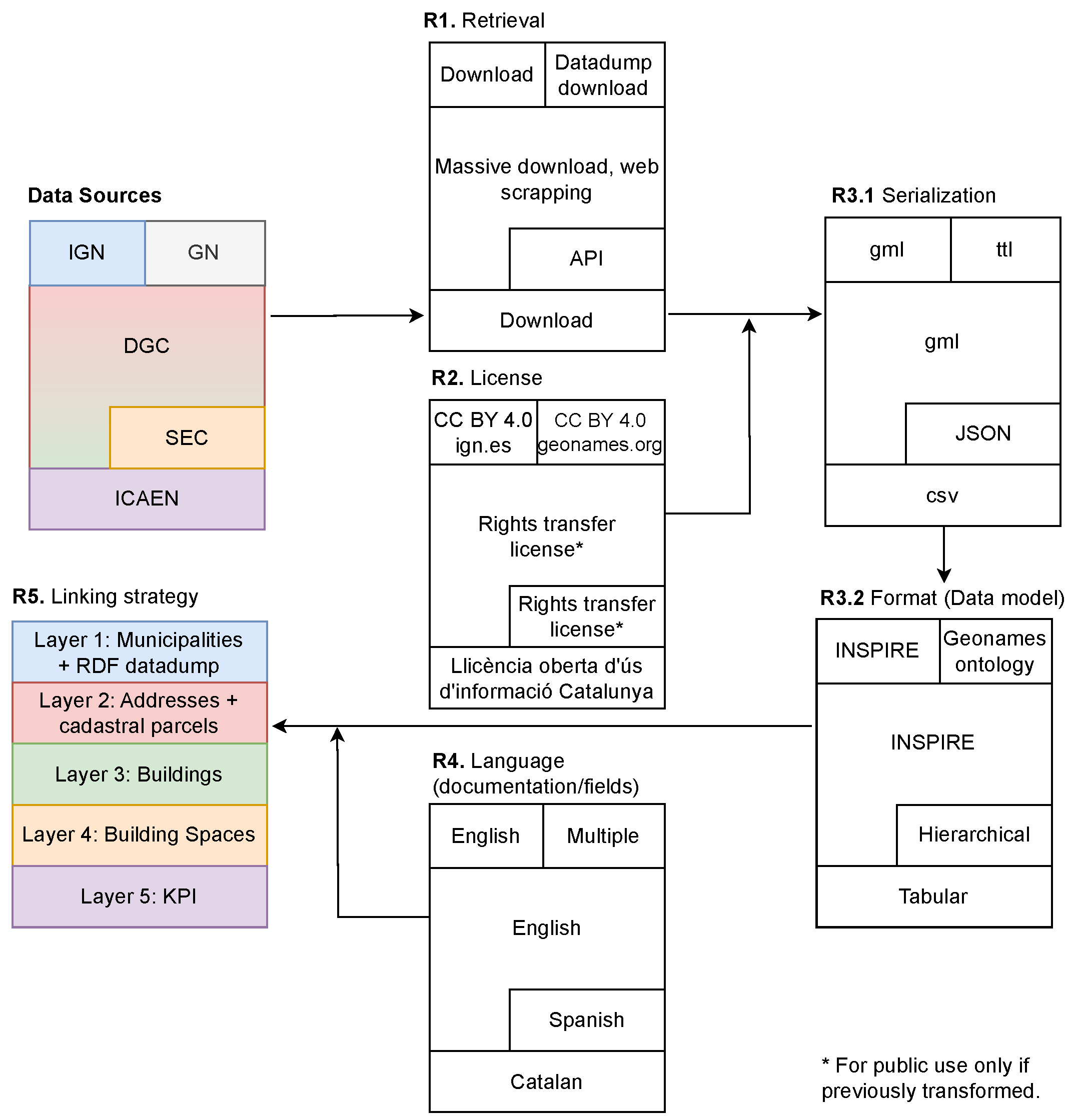
Data sources. The extracted variables from the previous step or a previous iteration’s new requirements sustained the exploration task, which eventually led to pre-select potential data sets that contained these variables and met most of the data requirements. In the current case, beyond the data sets fixed by the project, to fulfil the UC’s specifications, an exploration process was driven to identify other data sources that were needed to enrich the Knowledge Graph (KG) and improve data linkage. A methodological asset containing a quick analysis of the selected data sets to check the above-listed data requirements compliance is depicted in Figure 2. Figure 3 represents the intended linkage with each selected data source’s contributions and serializations. In addition, the Table 2 lists the complaint data sets selected with an acronym defined for referencing purposes.

4.2. Identify

Extract. On the content level, multiple mechanisms were used for data extraction that depended on the data source’s available access points. Single or massive file downloads, Application Programming Interfaces (APIs) clients petitions, and web scrapping were used to extract the data. A visual depiction of the retrieval methods used per data source is presented in the R1 box of Figure 2. It is worth mentioning that the multiple geographical scales identified from the datasets influenced the current operation. For the Barcelona pilot, subsets were described in the Subset column of Table 2 from which only the DGC dataset was directly at the municipality scale. The remaining datasets required subsetting operations or, in the case of the SEC data source, placing multiple APIs calls to reach the desired scale. After the extraction operation, the repository contained a combination of detailed and limited documentation that was enriched during the analysis activity, e.g., by extracting samples from raw data sets.
Data analysis. Regarding each data set metadata, data schema, samples, specifications, and documentation, an analysis example of relevant information is provided next. The convergence of three different languages: English, Spanish and Catalan, together with four distinct serializations: ttl, gml, JavaScript Object Notation (JSON), and comma-separated values (csv), and four formats or data models: Geonames ontology, INSPIRE’s, the Catalonian building space level cadastral data (SEC)’s data model and tabular was detected in the data sets to be integrated. Much as some data sources offered access to their information in multiple serializations, we only listed the ones that comply with the R2 data requirement. This set of facts was put together in Figure 2.
For raw data content analysis, each data set’s attributes name, type, brief description, range and other data constraints were extracted and provided with comments regarding possible problems, unique identifiers, and potential pre-processing operations e.g., buildings envelope geometries might be reprojected from the EPSG:25829 to CRS84 and convert it to Well-Known Text (WKT) format. Descriptive statistics were applied when possible to each iteration’s selected features. The number of blank or null cells counted supported the decision about which data set’s feature series to keep or discard e.g., the Catalonian Buildings Performance Certifications data (ICAEN) data set has only half of its features covered, thereby deciding the partially covered features is not worth including at least for the current Use Case and iteration. For some data sets descriptive statistics was difficult before data integration was performed. This was the case of the DGC’s semi-structured data because addresses, parcels, and buildings information are compiled in separate files and packed per municipality. For brevity and because each feature’s analysis depended on the data set, a short example of these outputs is provided in Table 3.
Ontology requirements specification. Both the use case specification and the data analysis outputs fed the actors with information to define the purpose and scope of the ontology.
  • Purpose: to define an extendable core of clearly defined concepts needed for the buildings’ energy efficiency information geospatial analytics, which, being populated with multiple and heterogeneous data sources, could enable interoperability among them.
  • Scope: The scope is bounded by the energy Benchmarking Business Case. Nevertheless, the possibility of extending the vocabulary to other use cases is desired.
Then, a set of non-functional ontological requirements were listed.
  • Design patterns, Concepts, Attributes and Relationships from standardized and widely-used ontologies should be reused as much as possible
  • The Geographic Query Language for RDF Data (GeoSPARQL) standard should be supported i.e., reusing GeoSPARQL ontology concepts
  • The ontology should be implemented in Web ontology language 2 Description logics (DL) (OWL2DL)
A set of CARs tables was generated as the functional requirements main asset. Starting from the UC variables listed in Table 1 in each implementation iteration, the CARs tables were extended with details or entities, always prioritizing the ones that were involved in the corresponding iteration business questions answers. Besides other phases’ information, an example of this is depicted in Table 4.

4.3. Model

Resource naming strategy. Within the data analysis report, it was observed that entities such as the Cadastral Parcel (CP), Building (BU) and Building Space (BS) shared attributes such as their Address (AD) information, Administrative Unit (AU), and their national cadastral references were recognized as a common unique identifier present in some of the data sets. Such identifier and attributes’ linking potential are thus, the closing statement for R5 compliance. Provided that the cadastral reference can be used to formulate multiple entities’ URIs, a strategy was formulated on top of it in order to have the data sets containing these entities linked together.
Hence, data linkage was planned to be layer-based starting from broader to narrower geographical entities. The region’s AUs contain CPs that are associated with ADs and, in turn, contain BUs that enclose BSs. This linking strategy, which is represented in the last box of Figure 2, also provides a refinement mechanism for the previously-answered business questions. The URI minting strategy as seen in Table 5 was developed for ontological and shapes entities using the hash dereferencing recipe as the chosen one. Whereas, for resource entities and graphs the slash recipe was selected.
Ontology implementation and validation. To support ontology conceptualization, diagrams in the UML-like Chowlk notation [23] were created per iteration. Hence enabling a high-level communication canal between ontology developers and domain experts involved in the project. In the three first columns of the Table 4, it is possible to observe that conceptualization already started with the identification of the CARs. The remaining columns of the Table 4 show how the conceptualization was translated into triples with reused ontological terms.
In order to reuse these concepts, an exhaustive survey of existing ontologies in the domain was conducted, with priority given to well-maintained, widely used, and standardized concepts to comply with the first non-functional ontological requirement. In addition, the selection criteria for including or excluding non-standardized ontologies were based on the existence of alignments with the standards or with other widely used ontologies.
In the Table 6, the URIs corresponding to the proposed and reused ontologies with their prefixes are listed. Between hard and soft reuse, ontological resources’ soft reuse was the selected approach. When the existing ontologies’ concepts matched their definitions with those of the CARs conceptualized the decision was to adopt the existing concept. Whereas when the concepts differed in their definitions and/or were not present in the domain’s ontologies, they were created.
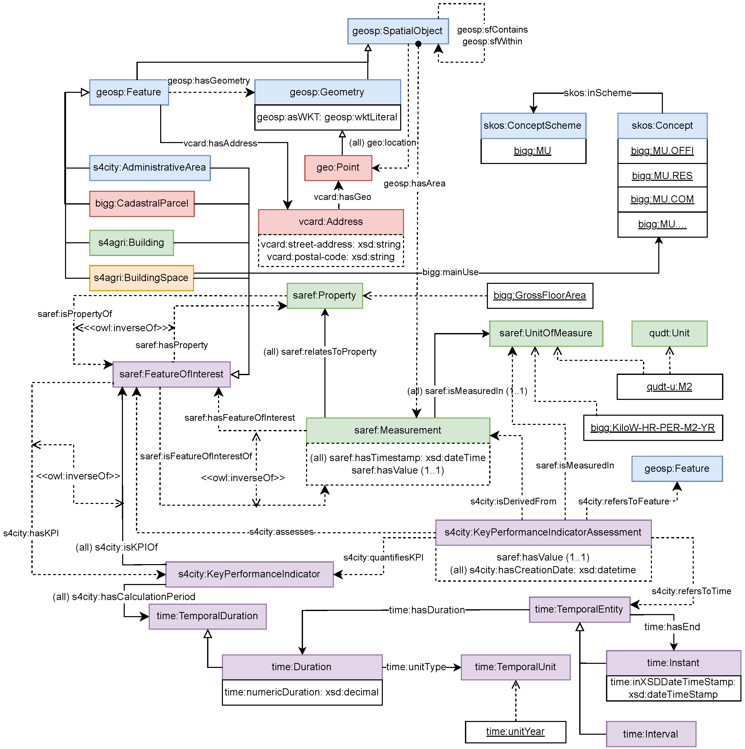
As a result, classes, properties, attributes, axioms, and hierarchies are depicted within Figure 4. It represents how the last implementation iteration of the ontology extended using the formulated linking strategy layers, which at the same time obey the same colour coding from Figure 2.
Multiple versions of conceptualization diagrams per iteration were created yet only the resulting one is shown and described below.
During the first iterations, the conceptualization was focused mainly on making geographic entities interoperable. Different options were considered to address distinct levels of administrative areas integration. Nevertheless, due to the second non-functional requirement suggested reusing the GeoSPARQL ontology, it was decided to implement their entities together with a well-known geographic design pattern. Plus, for the distinction between administrative levels, the Geonames Simple Knowledge Organization System (SKOS) features taxonomy was reused. Which also represents thinking one step ahead to LOD. Both Feature classes coming from the Geonames and GeoSPARQL ontologies are equivalent according to their documentation alignments; thus, an owl:equivalentClass statement was set between them. Apart from the previously mentioned ontologies reused the The Smart Applications REFerence ontology (SAREF) extension for Smart City (s4city) was reused. The variables related to location details for cadastral parcels are listed in the second row of the Table 1. The appearance of the cadastral parcel concept, which deferred the existing standard concepts, motivated the creation of one as a specialization of the GeoSPARQL Feature class using the BIGG project prefix. Despite having multiple options for the address-related concepts the decision to reuse the vCard Ontology for describing People and Organizations (vCard) vocabulary superseded others for its alignments to the standard business cards’ file format Virtual Contact File (vcf). A set of properties also were reused to support the geo:Point class which allows populating the ontology with a specific type of geometry. The red and blue colours represent the first and second layers of the linking strategy plan. In the upper left-hand side of Figure 4 the red boxes represent the classes that extended the geographic entities’ iteration model. Reused from the Extension of SAREF for the agriculture and food domain (s4agri), the main classes added in the subsequent iteration were the Building (BU) s4agri:Building class followed by the saref:Measurement. The reason why s4agri overtake others e.g., the SAREF extension for building (s4bldg) is because the way the Parcel, Building and Building Space classes are modelled is aligned with the geographic pattern used in the initial iterations which, in addition, it reuses GeoSPARQL classes. The red-coloured bigg:CadastralParcel box acts as linkage entities among two data sets i.e., there are sharing triples in distinct data sets’ graphs. Units of measure and property classes were also reused from the SAREF core ontology and the units’ instances were borrowed from the Quantities, Units, Dimensions, and Types Ontology (qudt) units vocabulary. In the lack of a definition regarding the gross floor area of a space, the bigg:GrossFloorArea was created as an instance of saref:Property. In order to integrate the KPIs coming from the ICAEN data set the ontology was extended by following the s4city extension logic and entities. Two were the classes that linked the data sets. Namely, s4agri:Building and s4agri:BuildingSpace instances connected the Catalonian municipalities INSPIRE cadastral data (DGC) data sets and those with the SEC and ICAEN data sets, respectively. Time features were included to attach each Key Performance Indicator Assessment (KPIa) to their corresponding date. Finally, provided that buildings’ main use types taxonomy depends on how each organization manages and classifies its goods, it represents a considerable challenge to provide good interoperability among the data sets. Data governance was agreed to prioritize governmental bodies’ information, and the finest geographical granularity was at the BS level; thus, a concept scheme was populated with the SEC data set building’s main use taxonomy concepts reusing the SKOS vocabulary. The addition of other data sets’ taxonomies was left for future iterations. The complete SEC taxonomy translated to SKOS entities is presented in Table 7. For covering the missing units in the qudt units vocabulary, two units of measure were created as instances of saref:UnitOfMeasure in the Terminological component statements (TBox) side.
In summary, most of the terms present in this study’s ontology make use of reused ontologies’ entities, only one class, one object property and seventeen ontology individuals were created along the four iterations as seen in the Table 7. It is noteworthy that the resource naming strategy was used in the formulation of them.
The implementation language used for the ontology encoding obeys OWL2DL as stated in the third non-functional requirement. This standard sub-language of the Web ontology language (OWL)2 full being decidable, supports Direct Semantics and covers the whole of the reused ontologies’ expresivities. The encoding operation was executed avoiding possible issues between the ontology concepts’ relationships or restrictions using the Protégé [24] editor’s importing tools. Thus, ensuring the conceptualization was properly encoded.
Both conceptualization and encoding sub-activities were complemented with metadata, e.g., versioning and licensing statements and hand-made instantiation examples in each iteration which served further on in the Convert and Publish phases. Listing 1 is an example of an ontological definition of an object property.
Listing 1. Example of an ontological definition of an object property.
1 ###  http://bigg−project.eu/ld/ontology#mainUse
2 bigg:mainUse rdf:type owl:ObjectProperty ;
3         rdfs:domain geosp:Feature ;
4         rdfs:range skos:Concept ;
5         rdfs:comment "To specify the main use of a space."@en ;
6         rdfs:label "main use"@en .
For ontology logical consistency checking purposes, the pre-installed Hermit reasoner acting on top of the Protégé editor supported the ontology validation by checking the inferred facts consistency. In addition, the OntOlogy Pitfall Scanner! (OOPS!) tool [25] allowed us to generate a validation report after checking the official RDF validator the World Wide Web Consortium (W3C) provides online [26]. The OOPS!’s validation report fed the developing team back to fix some small issues as described in the Maintain phase. At the end of each iteration, domain coverage was updated with the corresponding set of variables included in the iteration until the use case was solved. As stated before, the proposed methodology suggested splitting ontology evaluation in two, the current activity is complemented by ontology verification which takes part in the Enrich phase.

4.4. Convert

Pre-processing The very first sub-activity to transform each data set was pre-processing it. The data analysis report, as seen in Table 3, brought light into the kind of operations each data set feature required to generate the subject’s URIs, and to ensure the compliance of the ontology’s datatypes and formats. Those potential operations were revised and implemented with distinct approaches in function of the data set. For instance, buildings’ bi-dimensional envelope geometries from the DGC data sets collection serialized in gml were parsed, reprojected from the EPSG:25829 Spatial reference system (srs) to the CRS84 srs and formatted according to the WKT format to enable GeoSPARQL queries in a batch process using a combination of tools. In contrast, the ICAEN data set which consisted of a single table required a single run of simpler operations to move forward to the mapping sub-activity. Pre-processing operations for constructing URIs were not listed in the data analysis report until a resource naming strategy was defined. Each iteration provided more pre-processing operations that were applied to the variables of the iteration in turn. As a result, this process was conducted to have refined data ready to be mapped and materialized. The tools used for pre-processing were among others, OpenRefine (https://openrefine.org/) with its General Refine Expression Language (GREL), QGis (https://qgis.org/) for obtaining reprojections of geometries, and a set of Python’s (https://www.python.org/) libraries such as Pandas (https://pandas.pydata.org/) and GeoPandas (https://geopandas.org/). A simple example of the operations applied in batch to the DGC data sets’ address identifiers for minting administrative unit URIs suffixes is presented in the Listing 2.
Listing 2. A reusable pre-processing operation example in JSON that uses GREL generated with OpenRefine.
  1 [
  2  {
  3   "op": "core/column−addition",
  4   "engineConfig": {
  5    "facets": [],
  6    "mode": "record−based"
  7   },
  8   "baseColumnName": "gml:featureMember − AD:Address − gml:id",
  9   "expression": "grel:\"ES.SDGC.AU.\"+value.split(\".\")[3,5].join(\".\")",
10   "onError": "set−to−blank",
11   "newColumnName": "AdministrativeUnit",
12   "columnInsertIndex": 1,
13   "description": "Create column AdministrativeUnit at index 1 based on column
        gml:featureMember − AD:Address − gml:id using expression grel:\"ES.
       SDGC.AU.\"+value.split(\".\")[3,5].join(\".\")"
14  }
15 ]
Mapping and materialization. The mapping sub-activity, once again, varied from data set to data set. Nevertheless, what was common was the selected language, i.e., the triples-based RDF Mapping Language (RML), to be as close as possible to the W3C standard Relational Database (RDB) to RDF Mapping Language (R2RML). Multiple mapping files were generated per iteration following the ontology instantiation examples as the main assets to support above all, the conceptual part of the assertions. From the data content point of view, it was crucial to have direct access to the headers or features original names and data paths that served as pointers in the mapping code in order for the refined data to be materialized in RDF triples. An example of how the mapping files look is shown in Listing 3. Features’ paths, in combination with the resource naming strategy, the ontology assertions, and the objective graph URI together formed the mapping file that fed the materialization engine.
Listing 3. A mapping example in RML for generating AU entities.
  1 <#AdministrativeUnit>
  2
  3   a rr:TriplesMap ;
  4
  5   rml:logicalSource [
  6     rml:source "Data/DGC/Addresses/Refined/A.ES.SDGC.AD.08900.gml";
  7     rml:iterator "/gml:FeatureCollection/gml:featureMember" ;
  8     rml:referenceFormulation ql:XPath ;
  9   ] ;
10
11   rr:subjectMap [
12     rr:template "http://bigg−project.eu/ld/resource/
       AdministrativeArea/DGC−id−{AD:AdminUnitName/@gml:id}" ;
13     rr:class s4city:AdministrativeArea  ;
14     rr:graph graph:DGC ;
15   ] ;
16 .
Batch processing was configured when needed to make the selected engine run iteratively until populating the ontology with the data in scope. Despite having tried multiple engine options, the chosen one was morph-kgc (https://github.com/morph-kgc/morph-kgc) because of its good performance when dealing with big amounts of data, which allowed parallel processing.
Data validation. From the data analysis report asset, the preliminary data constraints identified were the starting point of this activity. A good number of restrictions were already considered while modelling the ontology. Although it is possible to validate data solely from the ontology statements through inference, the open-world assumption such an approach implies was not enough to ensure the compliance of the data against all of its constraints. For this, a semi-closed world was bounded by using the Shapes Constraint Language in shapes definitions automatically generated from the ontology. The tool used for this purpose was Astrea (https://astrea.linkeddata.es/) which basically translated ontology statements restrictions to ready-to-use triples any Shapes Constraint Language (SHACL) engine accepts as input for data validation. The Listing 4 is an extract of the automatically generated shapes that depicts one translation of the rdfs:range property to a node shape as an example.
Listing 4. An automatically generated SHACL shape example using Astrea in ttl for reporting missing type for a unit of measurement entity.
  1 ## −List of prefixes−
  2
  3 <https://astrea.linkeddata.es/shapes#db085280eb44e73456450bcaf4d931b0>
  4    a                     sh:PropertyShape ;
  5    rdfs:isDefinedBy  <https://saref.etsi.org/core/> ;
  6    rdfs:label          "is measured in"@en , "A relationship identifying the
      unit of measure used for a certain entity."@en ;
  7    sh:class             saref:UnitOfMeasure ;
  8    sh:description     "A relationship identifying the unit of measure used
      for a certain entity."@en ;
  9    sh:name             "is measured in"@en ;
10    sh:nodeKind         sh:BlankNodeOrIRI ;
11    sh:path             saref:isMeasuredIn~.
Passing the RDF data and the shapes file to a SHACL engine produced a validation report resembling the Listing 5 in this case with a non-compliant statement and the details of the non-conformity.
Listing 5. An automatically generated SHACL validation report example in ttl reporting missing type in a unit of measurement entity.
  1 # −List of prefixes−
  2
  3 [] a sh:ValidationReport ;
  4  sh:conforms false ;
  5  sh:result [ a sh:ValidationResult ;
  6    sh:focusNode <http://bigg−project.eu/ld/resource/Measurement/GFA−SC
       −id−BS.1317101DF3811E0001RO> ;
  7    sh:resultMessage "Value does not have class saref:UnitOfMeasure" ;
  8    sh:resultPath saref:isMeasuredIn ;
  9    sh:resultSeverity sh:Violation ;
10    sh:sourceConstraintComponent sh:ClassConstraintComponent ;
11    sh:sourceShape <https://astrea.linkeddata.es/shapes#
       db085280eb44e73456450bcaf4d931b0> ;
12    sh:value <http://qudt.org/vocab/unit/M2> ].
PySHACL (https://doi.org/10.5281/zenodo.7966546) was the selected engine because it is fully compliant with the SHACL W3C recommendations, its simple use, its reasoning capabilities and command line tools. Proper engine configuration allowed lifting most of these kinds of non-conformities by enabling inference with the ontology as an extra input.

4.5. Enrich

Load and inference. After data cleaning, the validated RDF data was generated in multiple N-Quads (nq) files which is a line-based plain text serialization of RDF that allows named graph encoding. It was identified that the selected materialization engine was unable to generate triples when, in the mapping files, some entities had nothing to map with, i.e., single-time assertions such as units, temporal or KPIs instances. These additional triples were manually coded and included in the raw RDF repository as an extra nq file. Appending all the generated nq files into a single one would result in data linkage, yet it is not feasible due to plain text can be expensive for storing, querying, reasoning, and performing other graph-based operations. Thus, an ingesting pipeline was configured to feed a selected triplestore for tackling these kinds of issues. There are multiple storage options available, but because of the second non-functional ontological requirement, the shortlisted candidates were the ones that had GeoSPARQL query support in their endpoints. owl:SameAs, inverse, and transitive inferencing as well as a SHACL validation were some additional features desired for the triplestore to be supported.
Covering most of the needs, the whole set of nq files was bulk-loaded in parallel threads (parsing, entity resolution, load and inference) to a local GraphDB (https://www.ontotext.com/products/graphdb/) repository. The architecture of the selected triplestore allowed loading the ontology code together with the validated data and with the proper configuration, inferencing was enabled as part of the loading process. Four are the OWL reasoning profiles supported by the selected triplestore. From these, the OWL2RL, a Rule Language (RL) enhanced OWL profile, was configured to cover most of the ontology expressibility for reasoning.
As a result, not only the asserted but also the inferred triples were totally materialized after the completion of the forward-chaining reasoning process and the semantic repository-building. By means of gathering the information stored within the repository, GraphDB enabled a SPARQL endpoint from which one could query and aggregate the data on demand. Figure 5 encloses the visualization provided by the triplestore to navigate the graph.
Ontology verification. To support the energy benchmarking potential the integration of the selected data sets have so far, the Listing 6 is a query formulated to demonstrate this fact by performing a BS level data extraction for a cross-sectional energy benchmarking analysis. This SPARQL query was optimized by making use subqueries and aggregates algebra [27].
Listing 6. Barcelona’s Gothic neighbourhood building spaces energy benchmarking example SPARQL query.
  1 SELECT DISTINCT ?BScadastralReference ?KPIaValue WHERE{
  2  ?CP a bigg:CadastralParcel;
  3    geosp:sfContains ?BU.
  4  ?BU a s4agri:Building;
  5    rdfs:label ?BUcadastralReference;
  6    geosp:sfContains ?BS.
  7  ?BS a s4agri:BuildingSpace;
  8    rdfs:label ?BScadastralReference;
  9    bigg:mainUse/skos:prefLabel "Residential".
10  ?KPIa a s4city:KeyPerformanceIndicatorAssessment;
11     s4city:quantifiesKPI/rdfs:label "Non renewable energy use intensity";
12     s4city:assesses ?BS;
13     saref:hasValue ?KPIaValue;
14     s4city:hasCreationDate ?KPIaDate.
15  FILTER (YEAR(?KPIaDate) = 2014 )
16  {
17   SELECT DISTINCT ?CP WHERE{
18     ?CP a bigg:CadastralParcel;
19      vcard:hasAddress/vcard:hasGeo/geosp:asWKT ?ADpoint.
20     FILTER (geof:sfWithin(?ADpoint, "POLYGON((2.170 41.385,2.171
       41.383,2.174 ...))"^^geosp:wktLiteral ))
21   }
22  }
23 }
A fair peer comparison lies in selecting BS with at least the same location or with similar climatic parameters, a similar use type, a size-normalized indicator and a fixed year of analysis. In this example, a geometry defined by Barcelona’s Gothic neighbourhood bounds the limits of this energy benchmarking study, only residential spaces were taken into account, the “Non-renewable energy use intensity" was the chosen KPI and it was performed using only the values from the year 2014. This query was formulated following the ontological paths from the three last iterations’ models. In Table 8, an extract of the results of the previous query is provided. The calculated median of these results represents the Benchmark against which any BS of similar characteristics can be compared.
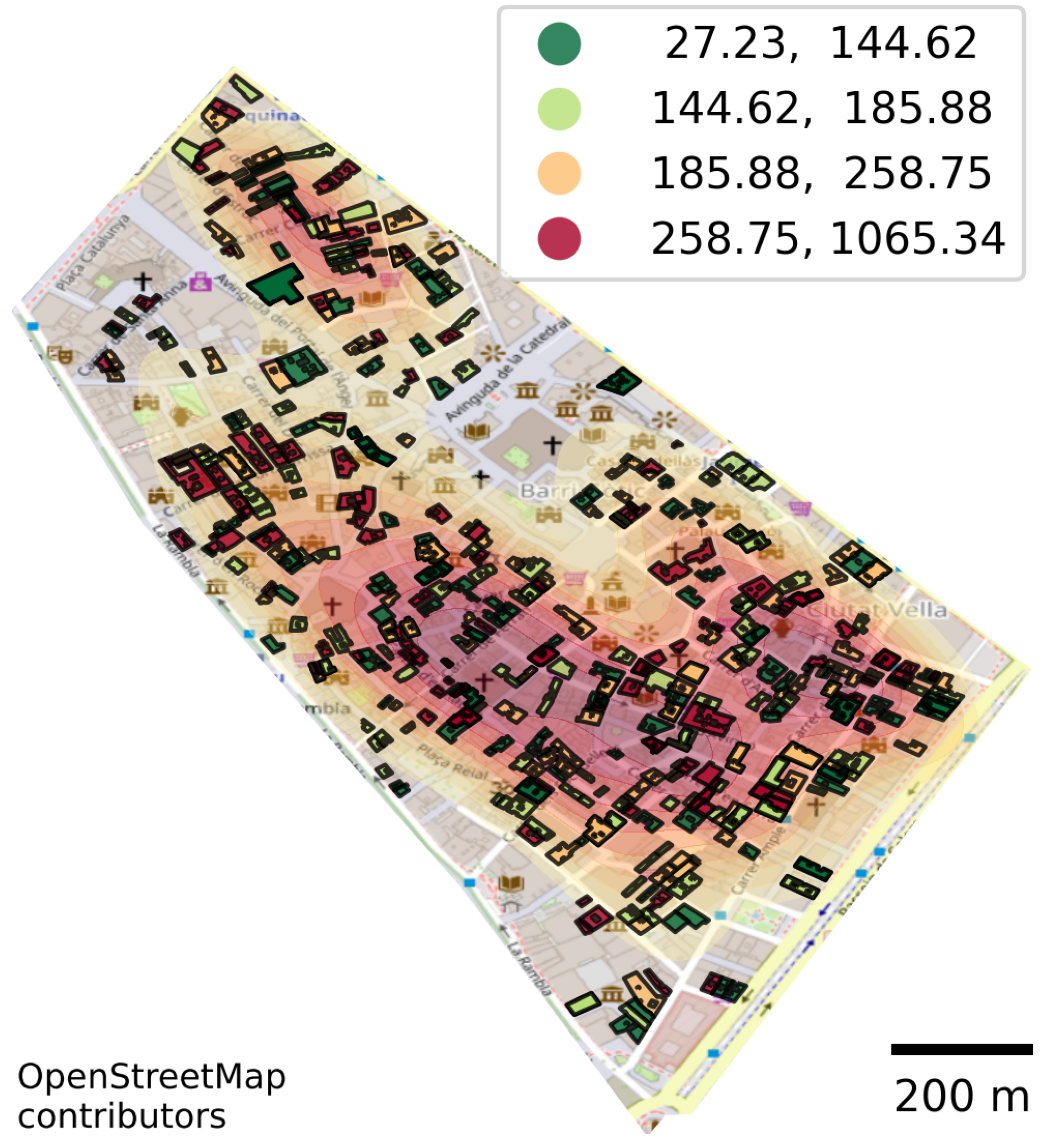
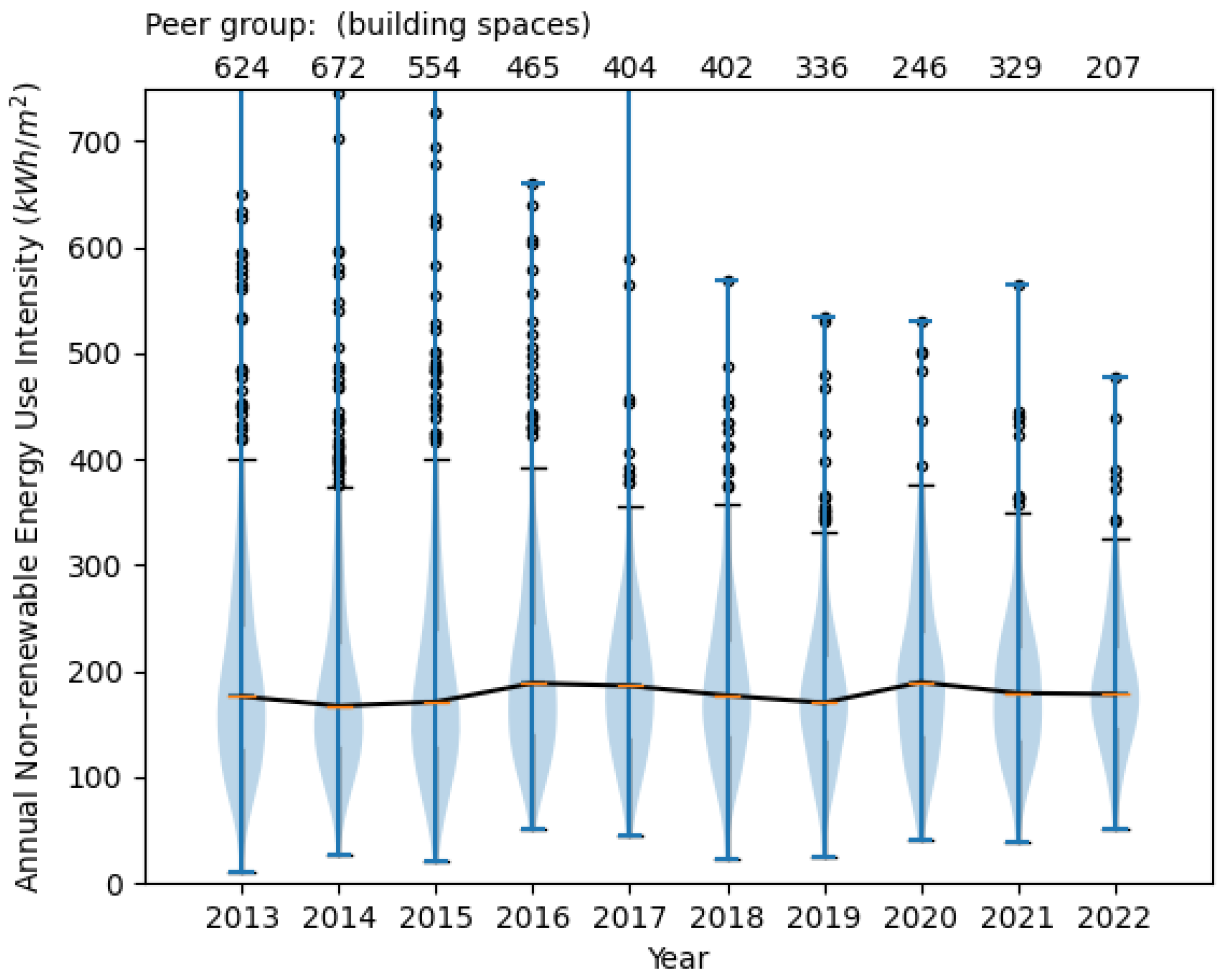
Finally, the tabular outputs were ported to external tools to generate Business Intelligence (BI) reports. Figure 6 is an example of a cross-sectional energy benchmarking histogram for Barcelona’s Gotic neighbourhood obtained from the values of Table 8. It is an artefact against which any residential building space energy performance from the zone can be compared. Figure 7 plots the polygons to represent the buildings within the mentioned neighbourhood that contain residential spaces with available KPIs values. The colour scale allows locating the worse performing residential BSs each BU has compared to other BUs. In addition, while not being an ontology requirement at this iteration, Figure 8 depicts a longitudinal energy benchmarking analysis performed over the BSs enclosed in the Gothic neighbourhood polygon on a yearly basis. In the figure, depicted as a violin plot, the circles represent outliers, the line indicates the median and the width of the shaded area represents the frequency distribution.
These figures were generated with a set of Python libraries that stores the SPARQL queries results (SPARQLWrapper (https://sparqlwrapper.readthedocs.io/)) in a geo data frame (geopandas (https://geopandas.org/)) and plot them into canvases (matplotlib (https://matplotlib.org/)). Similar figures were produced using distinct KPIs to complement the data validation reports into a final data set evaluation asset.
Linking. After putting the triples together for the first time, certain entities were identified as potentially linkable to other data sets. The geographical features entities generated after the first iteration corresponded to that of the Geonames Spain regions, Catalonian provinces and municipalities data (GN) data set. While working at a municipality level, a reconciliation against the scope region was driven using the OpenRefine tool with its RDF extension. The datatype properties containing the names of the municipalities from the Spanish administrative units’ geographical limits data (IGN) data set were compared against those of the GN data set with an automatic matching of 925 out of 948 entities. The remaining 23 entities were matched manually to ensure completeness. Listing 7 captured the automatic reconciliation operation which can be reused if future updates on the sources occur.
Listing 7. A reusable automatic reconciliation operation extract generated with OpenRefine.
  1 [
  2  {
  3   "op": "core/recon",
  4   "engineConfig": {
  5    "facets": [],
  6    "mode": "row−based"
  7   },
  8   "columnName": "http://www.w3.org/2000/01/rdf−schema#label",
  9   "config": {
10    "mode": "standard−service",
11    "service": "http://127.0.0.1:3333/extension/rdf−extension/services/gn−
       municipality",
12    "identifierSpace": "http://www.ietf.org/rfc/rfc3986",
13    "schemaSpace": "http://www.ietf.org/rfc/rfc3986",
14    "type": {
15     "id": "https://www.geonames.org/ontology#Feature",
16     "name": "https://www.geonames.org/ontology#Feature"
17    },
18    "autoMatch": true,
19    "columnDetails": [],
20    "limit": 0
21   },
22   "description": "Reconcile cells in column http://www.w3.org/2000/01/rdf−
      schema#label to type https://www.geonames.org/ontology#Feature"
23  }
24 ]
Later, the selected tool’s extension was configured to generate the owl:SameAs triples that linked the entities’ URIs.
As we wanted to keep instances for both data sources, the IGN municipalities entities were linked to that of DGC’s using the same approach. This time, both sets of instances belong to the just generated RDF data instead of external sources.
Afterwards, all the new triples were loaded into the triplestore whose reasoning engine inferred automatically owl:sameAs facts; thus, enabling querying information of a single entity from multiple URIs.

4.6. Publish

Ontology publication. During the project evolution, a version control system was used that at the same time acted as a publication repository (https://github.com/biggproject/Ontology/tree/v1.1/BIGGstd).
Linked data publication. After carefully analysing each source’s licensing statements, it has been decided not to enable an open access SPARQL endpoint, i.e., Linked Data (LD) access is only granted at the organization level for now. Nevertheless, all configurations for running a service were performed as recommended in a local environment. A simple authentication was programmed as the data access mechanism.

4.7. Exploit

Service platform development. One of the uncountable applications possible that could take profit from the linked BPC information and the INSPIRE geographical data can be visualized in Figure 9. Provided that data came from open sources, no mechanism for restricting access was formulated. The developed service platform was made open source in a GitHub repository (https://github.com/alexisimo/geobeb).

4.8. Maintain

Bug detection. From the Model phase on, each phase reported a number of bugs that were solved accordingly. To mention a few, incorrect prefixes definitions, URIs miss-typing, wrong relation between concepts, incorrect inference triples, malformed queries, invalid shapes formulation, incomplete auto-generated documentation, and platform-specific bugs were the most common bugs during the whole linked data cycle.
New requirement. With the evolution of the project and the communication established with the stakeholders, recurrent feedback was provided regarding what the requirements of each new iteration were. New concepts arose from discussions which also modified the evolution of the final LD data set as seen in Table 1. In the end, the need for new use cases was considered as ontology extensions to be developed in future and separate projects.

5. Discussion and Conclusions

This paper presented a novel methodology for generating Linked Data and its application in the energy benchmarking domain to address heterogeneous data integration and their geographical aggregation. The discussion and conclusions could be driven from two distinct points of view. First, from the methodological point of view, it was demonstrated through the building’s energy benchmarking use case results that the proposed methodology creates a logical data flow to achieve such a goal. Plus, it was validated that in contrast to other state-of-the-art methodologies, the one presented in this article has a sequential cycle which encourages an iterative and incremental design by incorporating ETL operations in its phases. Although the application of this methodology was demonstrated by a specific use case, any field that requires heterogeneous data sources integration could benefit from the current study. Nevertheless, just like any other methodologies, despite being agnostic to the tools and algorithms used in each phase, this methodology has automation challenges to deal with. By this time, only some independent tasks of the LD cycle have been fully automated. The complexity of each use case could have, makes difficult to generate a single and unique solution for data integration. Nevertheless, guides and tutorials on the present methodology are planned as part of future work.
Seccond, from the geographic aggregation point of view, a clear limitation of the current approach’s technology is the fact that the computation time required for querying data is proportional to the amount of data available in the delimited area chosen. Even when sub-querying in distinct scales it could only improve the performance slightly when dealing with massive amounts of data.However, thanks to the graph structure LD generated has, graph machine learning techniques such as Graph Neural Networks (GNN) or Knowledge Graph Embeddings (KGE) are unlocked to accomplish different tasks, which include but are not limited to, node classification, knowledge graph completion, graph classification, and graph generation. It is planned for future studies to explore such techniques to complete the BIGG knowledge graph generated with predicted KPIs.
A demonstration of the formulation of accessing policies reusing the ODRL model is part of a future work in which data integration is performed over not only open but private data sources. How a user can take profit from LD generated to extract geographically delimited data and cast aggregated KPIs normalized by what the geometry boundaries represent is also future work.

Author Contributions

Conceptualization, E.A.M.-S., E.G., J.C., R.G. and S.D.; Methodology, E.A.M.-S.; Software, E.A.M.-S.; Investigation, E.A.M.-S., J.M.B. and E.G.; Writing—original draft, E.A.M.-S.; Writing—review & editing, E.A.M.-S., J.M.B., E.G., J.C., R.G. and S.D.; Supervision, E.G., R.G. and S.D.; Project administration, J.C. All authors have read and agreed to the published version of the manuscript.

Funding

Thanks to the Spanish Award Centro de Excelencia «Severo Ochoa» en el marco del Plan Estatal de Investigación Científica y Técnica y de Innovación 2017–2020 with reference code: CEX2018-000797-S.

Data Availability Statement

The original contributions presented in the study are included in the article, further inquiries can be directed to the corresponding author.

Conflicts of Interest

The authors declare no conflict of interest.

Abbreviations

ADAddress
APIApplication Programming Interface
AUAdministrative Unit
BIGGBuilding Information aGGregation, harmonization and analytics platform
BPCBuildings Performance Certification
BSBuilding Space
BUBuilding
CARConcept, Attribute and Relationship
CPCadastral Parcel
DGCCatalonian municipalities INSPIRE cadastral data
DLDescription logics
ETLExtract Transform and Load
GeoSPARQLGeographic Query Language for RDF Data
GISGeographic Information System
gmlgeography markup language
GNGeonames Spain regions, Catalonian provinces and municipalities data
GRELGeneral Refine Expression Language
ICAENCatalonian Buildings Performance Certifications data
IGNSpanish administrative units’ geographical limits data
INSPIREInfrastructure for spatial information in Europe
JSONJavaScript Object Notation
KPIaKey Performance Indicator Assessment
KPIKey Performance Indicator
LDLinked Data
LODLinked Open Data
nqN-Quads
ODRLOpen Digital Rights Language
OOPS!OntOlogy Pitfall Scanner!
OWLWeb ontology language
qudtQuantities, Units, Dimensions, and Types Ontology
RDFResource Description Framework
RLRule Language
RMLRDF Mapping Language
s4agriExtension of SAREF for the agriculture and food domain
s4citySAREF extension for Smart City
SAREFThe Smart Applications REFerence ontology
SECCatalonian building space level cadastral data Sede Electrónica de Catastro
SHACLShapes Constraint Language
SKOSSimple Knowledge Organization System
SPARQLSPARQL Protocol and RDF Query Language
srsSpatial reference system
SWSemantic Web
ttlturtle
UCUse Case
URIUniform Resource Identifier
W3CWorldWide Web Consortium
WKTWell-Known Text

References

  1. Granderson, J.; Piette, M.; Rosenblum, B.; Hu, L. Energy Information Handbook: Applications for Energy-Efficient Building Operations; Lawrence Berkeley National Laboratory: Berkeley, CA, USA, 2011.
  2. de la Rue du Can, S.; Sathaya, J.; Price, L.; Mcneil, M. Energy Efficiency Indicators Methodology Booklet; Berkeley Lab: Berkeley, CA, USA, 2010; p. 71.
  3. Pérez-Lombard, L.; Ortiz, J.; González, R.; Maestre, I.R. A review of benchmarking, rating and labelling concepts within the framework of building energy certification schemes. Energy Build. 2009, 41, 272–278. [Google Scholar] [CrossRef]
  4. Abu Bakar, N.N.; Hassan, M.Y.; Abdullah, H.; Rahman, H.A.; Abdullah, M.P.; Hussin, F.; Bandi, M. Energy efficiency index as an indicator for measuring building energy performance: A review. Renew. Sustain. Energy Rev. 2015, 44, 1–11. [Google Scholar] [CrossRef]
  5. Haas, R. Energy efficiency indicators in the residential sector. Energy Policy 1997, 25, 789–802. [Google Scholar] [CrossRef]
  6. Khoshbakht, M.; Gou, Z.; Dupre, K. Energy use characteristics and benchmarking for higher education buildings. Energy Build. 2018, 164, 61–76. [Google Scholar] [CrossRef]
  7. Chung, W. Review of building energy-use performance benchmarking methodologies. Appl. Energy 2011, 88, 1470–1479. [Google Scholar] [CrossRef]
  8. Arjunan, P.; Poolla, K.; Miller, C. EnergyStar++: Towards more accurate and explanatory building energy benchmarking. Appl. Energy 2020, 276, 115413. [Google Scholar] [CrossRef]
  9. Vaisi, S.; Firouzi, M.; Varmazyari, P. Energy benchmarking for secondary school buildings, applying the Top-Down approach. Energy Build. 2023, 279, 112689. [Google Scholar] [CrossRef]
  10. Ali, U.; Shamsi, M.H.; Bohacek, M.; Purcell, K.; Hoare, C.; Mangina, E.; O’Donnell, J. A data-driven approach for multi-scale GIS-based building energy modeling for analysis, planning and support decision making. Appl. Energy 2020, 279, 115834. [Google Scholar] [CrossRef]
  11. Pauwels, P.; Zhang, S.; Lee, Y.C. Semantic web technologies in AEC industry: A literature overview. Autom. Constr. 2017, 73, 145–165. [Google Scholar] [CrossRef]
  12. Mathew, P.A.; Dunn, L.N.; Sohn, M.D.; Mercado, A.; Custudio, C.; Walter, T. Big-data for building energy performance: Lessons from assembling a very large national database of building energy use. Appl. Energy 2015, 140, 85–93. [Google Scholar] [CrossRef]
  13. Pasquinelli, A.; Agugiaro, G.; Chiara Tagliabue, L.; Scaioni, M.; Guzzetti, F. Geo-Information Exploiting the Potential of Integrated Public Building Data: Energy Performance Assessment of the Building Stock in a Case Study in Northern Italy. ISPRS Int. J. Geo-Inf. 2019, 8, 27. [Google Scholar] [CrossRef]
  14. Radulovic, F.; Poveda-Villalón, M.; Vila-Suero, D.; Rodríguez-Doncel, V.; García-Castro, R.; Gómez-Pérez, A. Guidelines for Linked Data generation and publication: An example in building energy consumption. Autom. Constr. 2015, 57, 178–187. [Google Scholar] [CrossRef]
  15. Zhang, Y.Y.; Hu, Z.Z.; Lin, J.R.; Zhang, J.P. Linking data model and formula to automate KPI calculation for building performance benchmarking. Energy Rep. 2021, 7, 1326–1337. [Google Scholar] [CrossRef]
  16. Li, Y.; García-Castro, R.; Mihindukulasooriya, N.; O’Donnell, J.; Vega-Sánchez, S. Enhancing energy management at district and building levels via an EM-KPI ontology. Autom. Constr. 2019, 99, 152–167. [Google Scholar] [CrossRef]
  17. Luo, N.; Pritoni, M.; Hong, T. An overview of data tools for representing and managing building information and performance data. Renew. Sustain. Energy Rev. 2021, 147, 111224. [Google Scholar] [CrossRef]
  18. Penteado, B.E.; Maldonado, J.C.; Isotani, S. Methodologies for publishing linked open government data on the Web: A systematic mapping and a unified process model. Semant. Web 2023, 14, 585–610. [Google Scholar] [CrossRef]
  19. W3C. Best Practices for Publishing Linked Data. 2014. Available online: https://www.w3.org/TR/2014/NOTE-ld-bp-20140109/ (accessed on 6 November 2023).
  20. Poveda-Villalón, M.; Fernández-Izquierdo, A.; Fernández-López, M.; García-Castro, R. LOT: An industrial oriented ontology engineering framework. Eng. Appl. Artif. Intell. 2022, 111, 104755. [Google Scholar] [CrossRef]
  21. Sequeda, J.F.; Briggs, W.J.; Miranker, D.P.; Heideman, W.P. A Pay-as-You-Go Methodology to Design and Build Enterprise Knowledge Graphs from Relational Databases; Springer International Publishing: Berlin/Heidelberg, Germany, 2019; Volume 11779 LNCS, pp. 526–545. [Google Scholar] [CrossRef]
  22. Best Practice Recipes for Publishing RDF Vocabularies. Available online: https://www.w3.org/TR/swbp-vocab-pub/ (accessed on 16 May 2023).
  23. Chávez-Feria, S.; García-Castro, R.; Poveda-Villalón, M. Chowlk: From UML-Based Ontology Conceptualizations to OWL. In Proceedings of the Semantic Web, Crete, Greece, 29 May–2 June 2022; Groth, P., Vidal, M.E., Suchanek, F., Szekley, P., Kapanipathi, P., Pesquita, C., Skaf-Molli, H., Tamper, M., Eds.; Springer: Cham, Switzerland, 2022; pp. 338–352. [Google Scholar]
  24. Musen, M.A. The protégé project. AI Matters 2015, 1, 4–12. [Google Scholar] [CrossRef] [PubMed]
  25. Poveda-Villalón, M.; Gómez-Pérez, A.; Suárez-Figueroa, M.C. OOPS! (OntOlogy Pitfall Scanner!): An On-line Tool for Ontology Evaluation. Int. J. Semant. Web Inf. Syst. (IJSWIS) 2014, 10, 7–34. [Google Scholar] [CrossRef]
  26. Prud’hommeaux, E.; Lee, R. W3C RDF Validation Service. 2004. Available online: http://www.w3.org/RDF/Validator (accessed on 27 June 2023).
  27. Kaminski, M.; Kostylev, E.V.; Grau, B.C. Semantics and expressive power of subqueries and aggregates in SPARQL 1.1. In Proceedings of the International World Wide Web Conferences Steering Committee, Montréal, QC, Canada, 11–15 April 2016; pp. 227–237. [Google Scholar] [CrossRef]
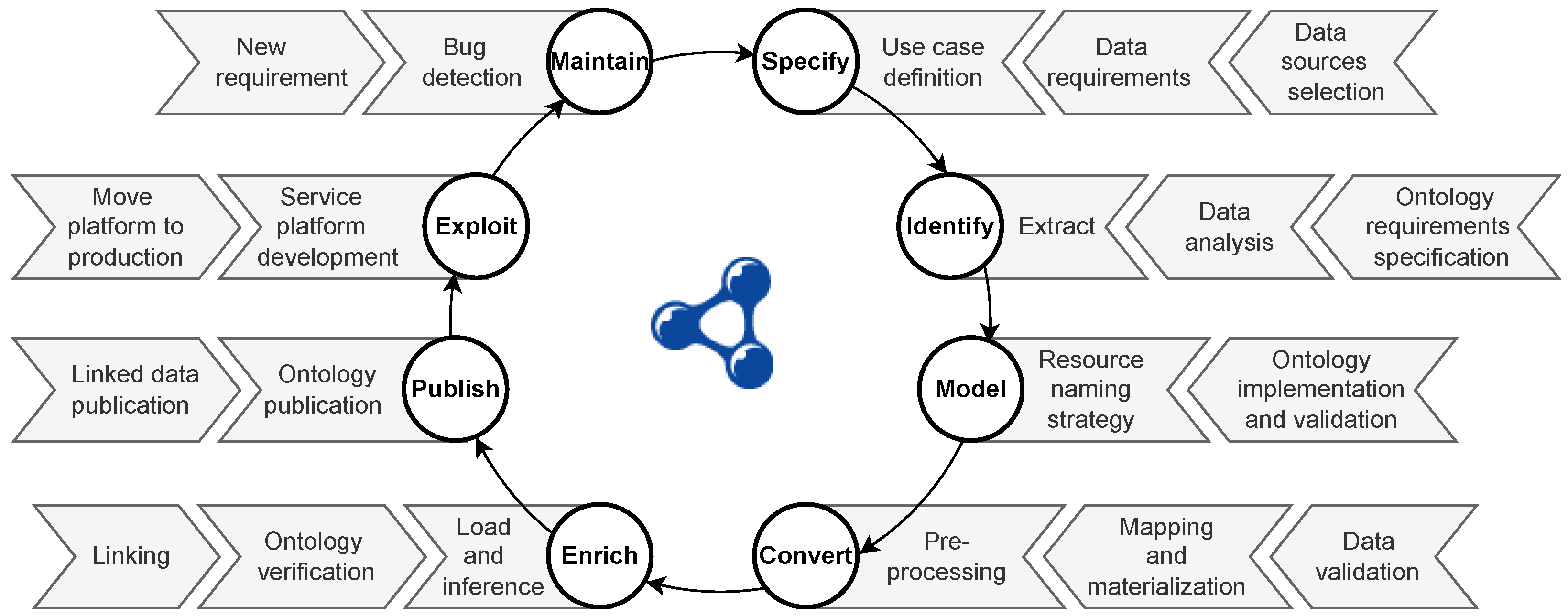
Figure 1. Linked data generation methodology’s cycle proposed.
Energies 17 03006 g001
Figure 2. Data requirements compliance check in brief.
Energies 17 03006 g002
Figure 3. Selected data sources’ main contributions and serializations.
Energies 17 03006 g003
Figure 4. Ontology conceptualization.
Energies 17 03006 g004
Figure 5. GraphDB graphical representation of a set of nodes and edges of the LD generated.
Energies 17 03006 g005
Figure 6. Barcelona’s Gothic neighbourhood residential building spaces cross-sectional energy benchmarking histogram in 2014.
Energies 17 03006 g006
Figure 7. Map of the neighbourhood’s worst-performing residential building space per building in 2014 (unit: kWh/m2).
Energies 17 03006 g007
Figure 8. Longitudinal Benchmarking of the Barcelona’s Gothic neighbourhood residential building spaces non-renewable energy use intensity.
Energies 17 03006 g008
Figure 9. Linked data exploitation demonstration. Geographically aggregated Buildings Energy Benchmarking tool.
Energies 17 03006 g009
Table 1. Variables identified within the Use Case and their implementation iteration.
UC VariablesIteration
Administrative area, Province, Municipality, Geometry1
Address, Postal code, Parcel, Location2
Building, Measurement, Gross floor area3
Building space, KPI, Energy label, Non-renewable primary energy consumption, CO2 emissions, CO2 label, Energy use intensity, Building spaces use type, Mixed-use buildings types proportion, KPI creation date-time4
Table 2. Data sets description and their implementation iterations.
AcronymDescriptionData Set Available inSubsetIteration
IGNSpanish administrative units’ geographical limits dataSingle compressed fileSingle gml file with fourth order administrative data1, 2
GNGeonames Spain regions, Catalonian provinces and municipalities dataSingle compressed data dumpFour ttl Catalonian administrative units geonames features1
DGCCatalonian municipalities INSPIRE cadastral data2841 compressed files5 gml files for the Barcelona pilot, one per INSPIRE theme2, 3, 4
ICAENCatalonian Buildings Performance Certifications dataSingle fileTabular file containing more than 1.3 M entries4
SECCatalonian building space level cadastral dataMultiple filesOne per Building Space totalling more than 2 M entries4
Table 3. Limited example of raw data analysis.
Data SetAttributeData TypeOriginal DescriptionComments
IGNsrsNameStringsrsThe whole data set’s geometries is in the EPSG:4258 srs. It might require reprojecting and transforming to WKT.
GNpostalCodeIntegerPostal codeRange from 10,000 to 45,000
DGCcurrentUseStringEs el uso dominante del edificio.Building’s use taxonomy: 1_residential, 2_agriculture, 3_industrial, 4_1_office, 4_2_retail, 4_3_publicServices.
ICAENADREÇAStringNom del carrerStreet address information available only in Catalan language. Might require a splitting operation.
SECsfcIntegerSuperficie del elemento o elementos constructivos asociados al cargo.Surface area. Range unknown before data integration.
Table 4. Use case vs. Reused Concepts, Attributes and Relationships (CARs) example.
Use CaseReused
VariableRelationTargetConceptRelationTarget
MunicipalitycontainsCadastral Parcels4city: AdministrativeAreageosp: containsbigg: CadastralParcel
Gross floor areahasValuefloatsaref: Measurementsaref: hasValuexsd: float
Building spacehasAreaGross floor areas4agri: BuildingSpacegeosp: hasAreasaref: Measurement
Building space use typetypetaxonomybigg: MUrdf: typeskos: ConceptScheme
Table 5. URI minting.
Base DomainPathsPatternsPrefix
http://bigg-project.eu/ld/ontology#  [className]bigg:
[propertyName]
resource/[className]/[identifier]bigg-res:
graph/[graphName]graph:
shapes#[shapeName]bigg-sh:
Table 6. Ontologies and misc vocabularies prefixes.
Table 7. New ontological entities generated.
TypeOntological EntityDefinition
owl:Classbigg:CadastralParcelAreas defined by cadastral registers or equivalent.
owl:ObjectPropertybigg:mainUseTo specify the main use of a space.
saref:Propertybigg:GrossFloorAreaGross floor area.
saref:UnitOfMeasurebigg:KiloW-HR-PER-M2-YRThe kilowatt hour per square meter year is a unit most commonly known as a unit for energy use intensity assessment of buildings.
saref:UnitOfMeasurebigg:KiloGMCO2-PER-M2-YRThe kilogram of carbon dioxide equivalent per square meter year is a unit most commonly known as a unit for carbon emissions assessment of buildings.
skos:ConceptSchemebigg:MUConcept scheme grouping main uses of spaces according to the Spanish Cadastral Electronic Site.
skos:Conceptbigg:MU.CLTCultural.
bigg:MU.COMComercial.
bigg:MU.ENTEntertainment.
bigg:MU.HLTCHHealth and charity.
bigg:MU.INDIndustrial.
bigg:MU.LEHOSLeisure and hospitality.
bigg:MU.OFFIOffice.
bigg:MU.RELReligious.
bigg:MU.RESResidential.
bigg:MU.SGLRSingular.
bigg:MU.SPTSports.
bigg:MU.STPKStorage-parking.
bigg:MU.URBWUrbanization works.
Table 8. Barcelona’s Gothic neighbourhood residential building spaces energy benchmarking example SPARQL query results. Cadastral references are hidden for privacy protection.
BS Cadastral ReferenceKPIa Value
“141...1DF3811C00..PE”“175.16”⌃⌃xsd:float
“101...9DF3811E00..PO”“258.4”⌃⌃xsd:float
“101...4DF3811E00..UA”“183.8”⌃⌃xsd:float
Disclaimer/Publisher’s Note: The statements, opinions and data contained in all publications are solely those of the individual author(s) and contributor(s) and not of MDPI and/or the editor(s). MDPI and/or the editor(s) disclaim responsibility for any injury to people or property resulting from any ideas, methods, instructions or products referred to in the content.