Article

Intraday Electricity Price Forecasting via LSTM and Trading Strategy for the Power Market: A Case Study of the West Denmark DK1 Grid Region

by
Deniz Kenan Kılıç
1,*,
Peter Nielsen
1 and
Amila Thibbotuwawa
2,3
1
Department of Materials and Production, Aalborg University, Fibigerstræde 16, 9220 Aalborg, Denmark
2
Center for Supply Chain, Operations and Logistics Optimization, University of Moratuwa, Katubedda, Moratuwa 10400, Sri Lanka
3
Department of Transport Management and Logistics Engineering, University of Moratuwa, Katubedda, Moratuwa 10400, Sri Lanka
*
Author to whom correspondence should be addressed.
Energies 2024, 17(12), 2909; https://doi.org/10.3390/en17122909
Submission received: 16 May 2024 / Revised: 7 June 2024 / Accepted: 10 June 2024 / Published: 13 June 2024
(This article belongs to the Section C: Energy Economics and Policy)

Abstract

:
For several stakeholders, including market players, customers, grid operators, policy-makers, investors, and energy efficiency initiatives, having a precise estimate of power pricing is crucial. It is easier for traders to plan, purchase, and sell power transactions with access to accurate electricity price forecasting (EPF). Although energy production and consumption topics are widely discussed in the literature, EPF and renewable energy trading studies receive less attention, especially for intraday market modeling and forecasting. Considering the rapid development of renewable energy sources, the article highlights the significance of integrating the deep learning model, long short-term memory (LSTM), with the proper trading strategy for short-term hourly renewable energy trading by utilizing two different spot markets. Day-ahead and intraday markets are taken into account for the West Denmark grid region (DK1). The time series analysis indicates that LSTM yields superior results compared to other benchmark machine learning algorithms. Using the predictions obtained by LSTM and the recommended trading strategy, promising profit values are achieved for the DK1 wind and solar energy use case, which ensures future motivation to develop a general and flexible model for global data.

1. Introduction and Background

Over the last decade, there has been rapid growth in the use of renewable energy sources like wind and solar in many countries. Most electricity is sold on power exchanges, and in the spot market, the pricing for the day ahead is determined around noon on the day before the energy is delivered. In general, day-ahead markets are supported by intraday and balancing markets, which help manage unexpected occurrences and weather changes. Intraday market transactions can occur up to a few minutes before delivery and are organized as auctions or continuous trading. System operators supervise balancing markets to ensure supply and demand are ultimately aligned for system stability [1]
The price of electricity is mainly affected by a balance of supply and demand (https://www.nordpoolgroup.com/en/trading/Day-ahead-trading/Price-calculation/, accessed on 5 October 2023) [2], market design, outages of large power plants, weather [1,3], season, day time, historical prices, transmission congestion, cost of unit operation, participants’ bidding strategies, etc. [4,5,6,7].
Every day at a specific hour (Central European Time (CET)/Central European Summer Time (CEST)), the day-ahead power price for each hour of the following day is released and orders are created for buying or selling [8]. After opening positions at the day-ahead price, the next day one can close the positions at the intraday price. Day-ahead and intraday electricity markets are segments within the energy market that facilitate the trading and procurement of electricity for different time horizons [9]. Both day-ahead and intraday electricity markets are crucial in ensuring efficient trading of electricity. They help integrate renewable energy sources, manage grid operations, and allow market participants to adapt to changing conditions at different time horizons before electricity delivery. These markets collectively contribute to the overall stability, reliability, and cost-effectiveness of the electricity supply.
Having an accurate prediction of electricity prices is quite important for various entities, including market participants, consumers, renewable energy integration, grid operators, policy-makers, investors, and energy efficiency initiatives [10,11,12]. It helps to facilitate informed decision-making, risk management, cost savings, grid stability, and the transition to a more sustainable and efficient energy system [9,13].
Accurate electricity price forecasting (EPF) helps traders make informed decisions about buying, selling, and scheduling electricity transactions [14]. It enables them to optimize their trading strategies, manage risks, and maximize profits in energy markets [15].
Risk-constrained arbitrage trading strategies for Dutch short-term electricity markets are studied in [16], which combines rule-based trading policy, technical indicator features, data augmentation, and deep reinforcement learning to achieve positive profits. In [17], it is shown that machine learning models outperform statistical ones for the French, Belgian, German, Nordic, and American day-ahead markets. In [18], different methods, including neural network-based machine learning approaches, are compared to predict prices in the Turkish intraday market. The comparison indicates that neural network-based approaches provide better evaluation metric results. Artificial neural network (ANN)-based models for day-ahead price forecasting are analyzed in [19] to propose robust forecasting tools. In [20], different machine learning techniques, like support vector regression (SVR), random forest, deep neural network (DNN), and convolutional neural network (CNN), are employed to predict electricity price on the day-ahead market. In [1], forecasting the price spread between the intraday/balancing and day-ahead markets via econometric models is analyzed to maximize the profit for the Polish and German electricity markets.
The field of EPF has long been the subject of several experiments and approaches [12,14,15,17,21,22,23,24]. In [25], a taxonomy of electricity price modeling approaches includes multi-agent (e.g., agent-based, supply function equilibrium, etc.), fundamental (e.g., parameter rich fundamental, etc.), reduced-form (e.g., jump-diffusion, Markov regime-switching, etc.), statistical (e.g., regression models, generalized autoregressive conditional heteroskedasticity (GARCH), etc.), and computational intelligence (e.g., neural networks, support vector machine (SVM), etc.) model types.
In [26], the long short-term memory (LSTM) network is indicated to be a powerful model in financial time series like stock prices. LSTM, a deep learning model, is also advantageous for EPF due to its ability to effectively capture temporal dependencies, learn from sequential data, handle complex patterns, and adapt to different forecasting horizons [4,5,10,11,13,21,23,27,28,29,30,31].
Most of the energy forecasts in the literature consist of wind and solar energy production and consumption predictions [32]. EPF research has been gaining attention in recent years but there are still fewer studies compared to others [18], especially for intraday market modeling and forecasting [1,33,34]. Therefore, one of the main aims of this article is to contribute to filling the gap in the literature that contains fewer EPF studies [32] by predicting intraday market prices, specifically for the Danish electricity market.
The Danish electricity system is divided into two separate areas, West Denmark grid region (DK1) and East Denmark grid region (DK2) [9,35,36,37,38]. DK1 is connected to the continental European electricity system, whereas DK2 is linked to the Nordic electricity system, which includes Sweden, Norway, and Finland. In this study, the DK1 region seen in Figure 1 is focused on. The figure is taken from (https://energinet.dk/el/systemydelser/introduktion-til-systemydelser/oversigt-over-systemydelser/, accessed on 5 October 2023).
In addition to EPF, obtaining a positive profit [23] from DK1 renewable energy trading is another goal of this article. It is assumed that investors open a position on the day-ahead market and subsequently close the position on the intraday market. For this, hourly intraday electricity market prices for the DK1 case are predicted using LSTM, and then investments are made with the proposed trading strategy. With the rapid development of renewable energy sources [24,39,40,41,42,43,44,45], the article focuses on demonstrating the importance of combining an advanced machine learning model, appropriate trading strategy, and two different markets for short-term renewable energy trading. Combining machine learning and trading strategy for the DK1 local use case sets this study apart from other studies. The machine learning and trading strategy approaches of the proposed method can be easily altered. This flexible structure can be easily adapted for other use cases and is a candidate to provide positive profits.
The rest of this article is organized as follows: Section 2 examines the data, prediction, and trading methods. Section 3 presents the results. Section 4 discusses the results and indicates concluding remarks.

2. Data and Methods

2.1. Data

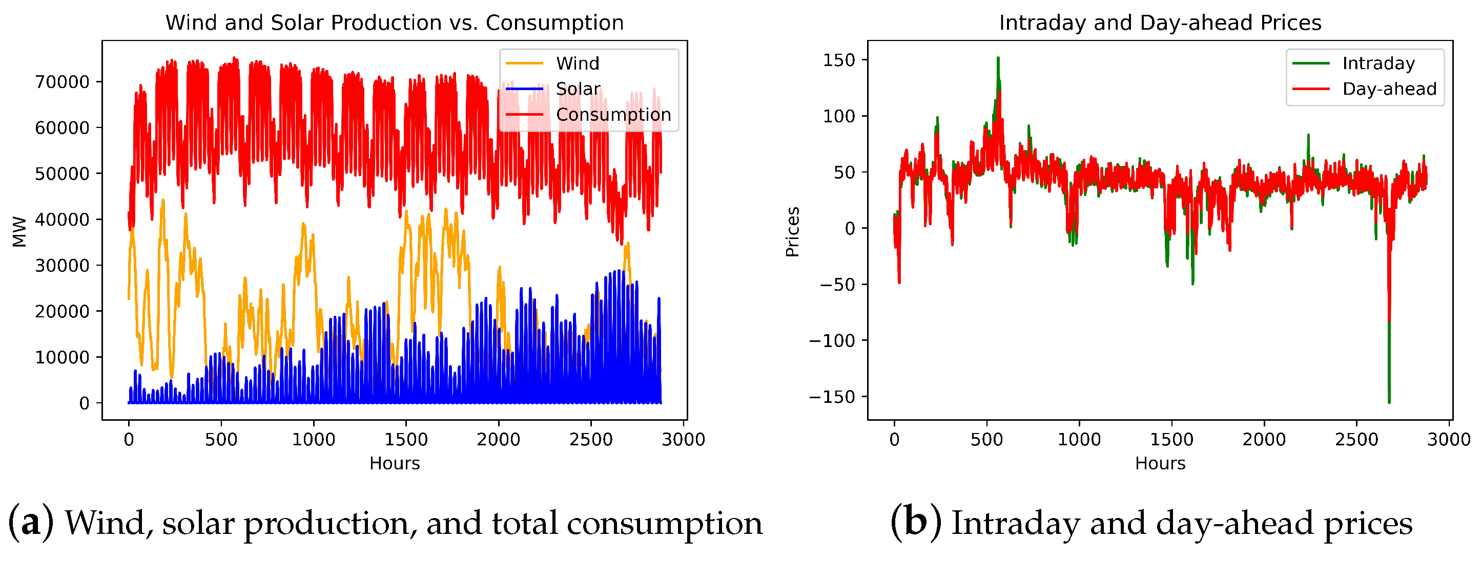
Data are collected from the Nord Pool (https://www.nordpoolgroup.com/, accessed on 12 April 2022), Energinet (https://energinet.dk/, accessed on 12 April 2022) and Energi Data Service (https://www.energidataservice.dk/, accessed on 12 April 2022) for the DK1 region. The combined data contain hourly forecast wind and solar production (megawatt (MW)), forecast total consumption (MW), and day-ahead and intraday market prices (euro (EUR)/megawatt-hour (MWh)) between 1 January 2019 and 30 April 2019.
Wind and solar electricity production, and total electricity consumption data are given on the left side of Figure 2. It is seen from the figure that consumption data show a clear seasonal pattern. In addition, intraday and day-ahead prices regarding these production and consumption data are shown on the right side of Figure 2.
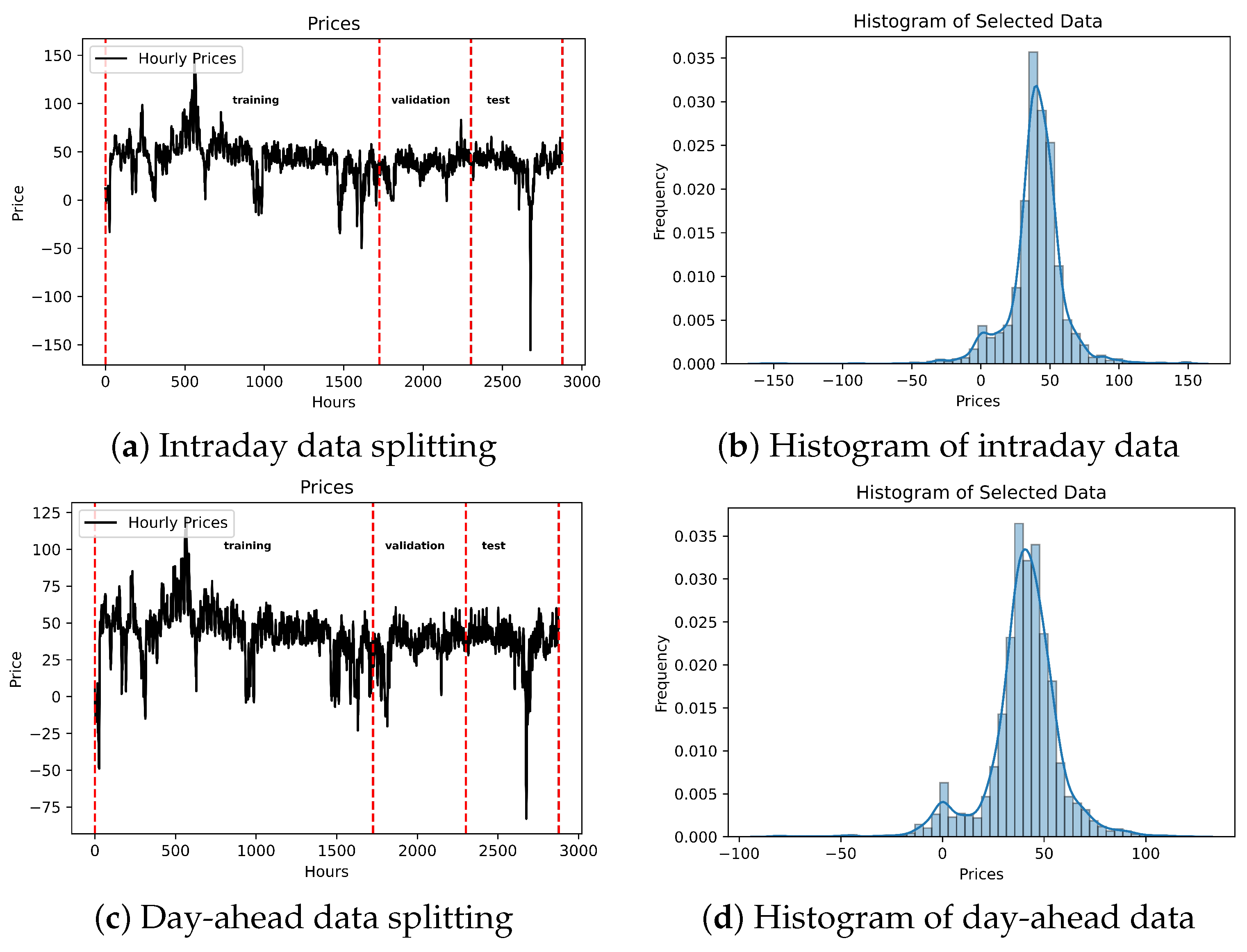
Descriptive statistics for intraday and day-ahead prices are given in Table 1. If the kurtosis values are considered, the kurtosis types are leptokurtic, i.e., the curve has a higher peak than the normal curve. Further, the data for both have more weight in the right tail of the distribution according to skewness scores.
Both intraday and day-ahead price data (length of 2877) are split into train, validation, and test sets. Almost 60% of all data are used in the train set (length of 1726), about 20% of all data are used in the validation set (length of 576), and nearly 20% of all data are used in the test set (length of 576). The data set is prepared as five variables with a one-time step as follows: solar power production (solar), wind power production (wind), total power consumption (cons), intraday market price (intraday), and day-ahead market price (day_ahead). By using a 1-ahead window set with five variables, the next hour’s intraday price is focused on being predicted. Splitting and histograms of the intraday and day-ahead price data are illustrated in Figure 3.

2.2. LSTM

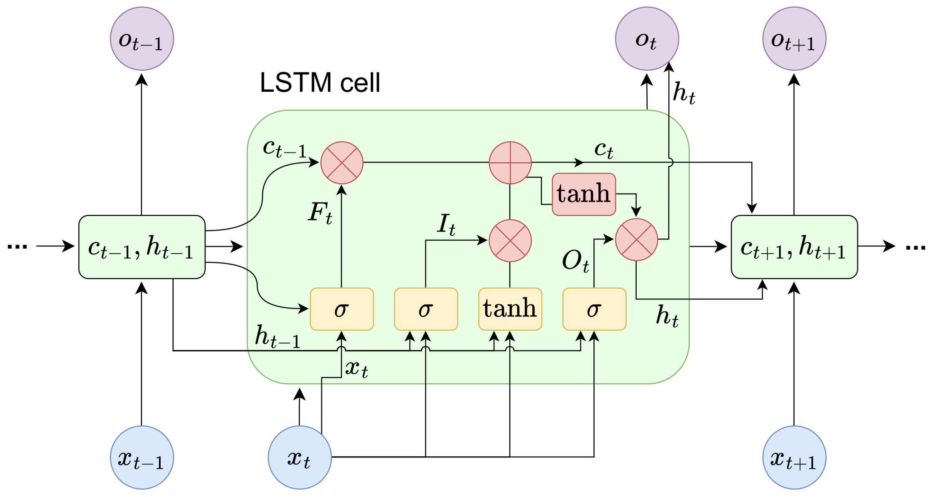
Due to fluctuations in energy costs over short and long periods, the network structure must include multiple memories for different time intervals. Therefore, this study utilizes LSTM, a recurrent neural network (RNN) type model, to predict intraday market prices. One unit LSTM is shown in Figure 4 [26].
The following equations are used to estimate the output h t of the memory cell at time t [46]:
F t = σ ( W F x t + U F h t 1 + b F ) ,
I t = σ ( W I x t + U I h t 1 + b I ) ,
C ˜ t = t a n h ( W C x t + U C h t 1 + b C ) ,
C t = F t C t 1 + I t C ˜ t ,
O t = σ ( W O x t + U F h t 1 + b O ) ,
h t = O t t a n h ( C t ) ,
where x t is an input vector to the LSTM at time t, the Ws and Us are weight matrices of the input and recurrent connections, the bs are bias vectors, h t in (6) is the output vector of the LSTM cell, C t in (4) and C ˜ t in (3) are state and candidate state vectors, respectively, F t in (1) retains the forget gate values, I t in (2) contains input gate values, and O t in (5) includes output gate values.

2.3. Trading Strategy

It is assumed that information regarding power production and consumption is available before deciding to enter the day-ahead market. Furthermore, it is possible to short-sell at the day-ahead price. For each hour, investors have the option to purchase or sell at the known day-ahead price. It is also possible to not participate in trading during a specific hour. Using these assumptions, the trading strategy is given in Equation (7).
P r o f i t = i n t r a d a y d a y _ a h e a d , i f i n t r a d a y _ p r e d > d a y _ a h e a d , d a y _ a h e a d i n t r a d a y , i f i n t r a d a y _ p r e d < d a y _ a h e a d , 0 , o t h e r w i s e .
The trading strategy states that if the predicted intraday price is higher than the day-ahead price, then the trader buys at the day-ahead price and sells at the intraday price. If the predicted intraday price is less than the day-ahead price, then the trader short-sells at the day-ahead and buys at the intraday. If they are equal then the trader does not trade. The profits of the best scenario are calculated as well to compare with the profits that are based on our predictions. The profits in the best-case scenario are determined by the difference between the day-ahead and intraday prices based on the observed values, i.e., they are greater than or equal to 0.
Note that since the main focus of this study is intraday market forecasting, the assumed trading strategy indicates that traders can buy or sell at the known day-ahead price for each hour. However, in the real day-ahead market, traders usually submit bids beforehand, and the auction results depend on whether the bid prices are higher or lower than the clearing price. In practice, traders need to predict both day-ahead and intraday prices before the auction and make decisions about where to place their bids in the market based on these forecasts.

3. Results

3.1. LSTM Predictions

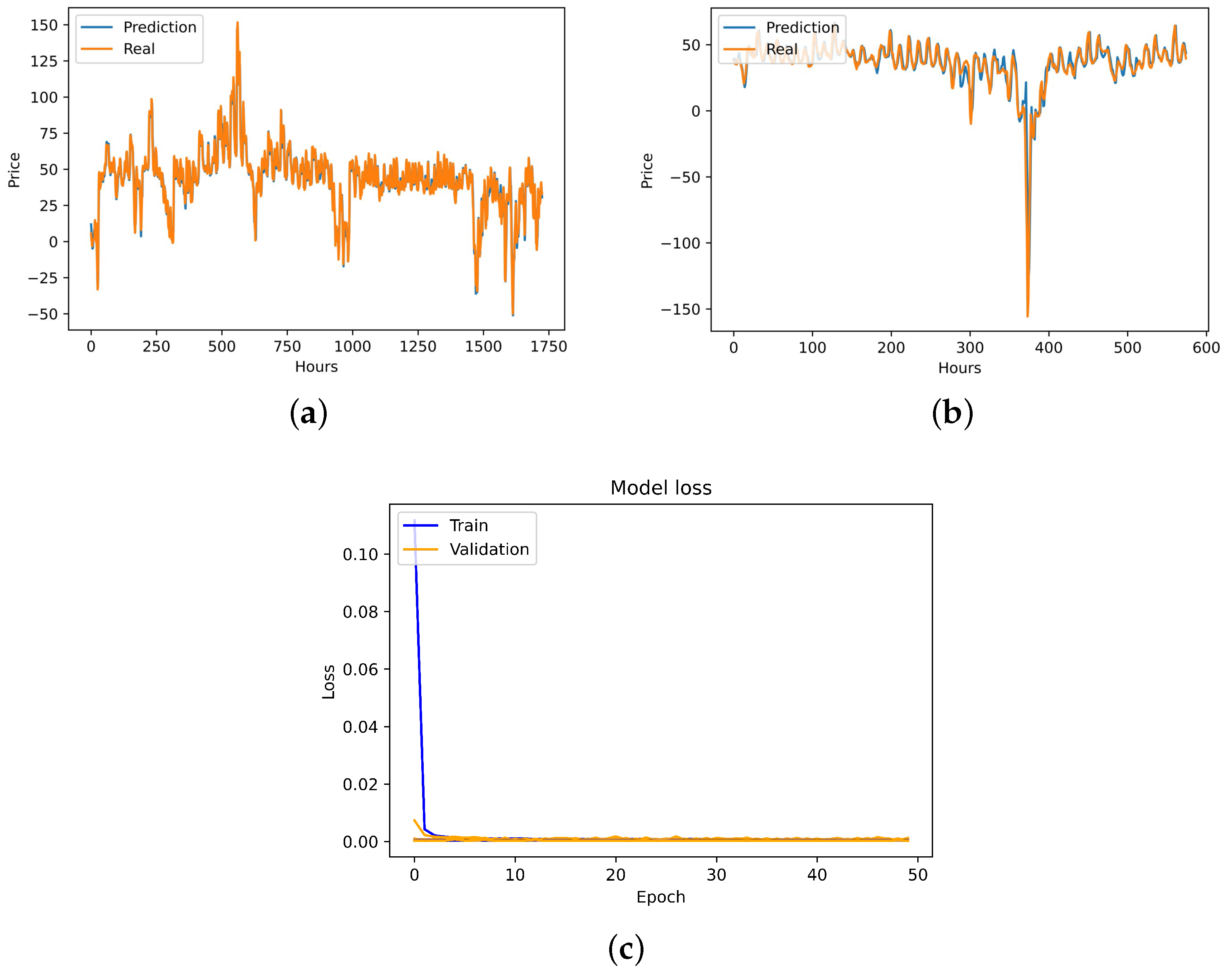
Random search and Bayesian optimization methods are employed for hyperparameter tuning of the LSTM parameter sets that are given in Table A1. Two hidden layers are used, where the first one is formed of 16 LSTM nodes and the second one consists of 128 nodes of a regular densely connected neural network. In the LSTM part, kernel, recurrent, and bias regularizers are put into practice. Batch normalization and rectified linear unit (ReLU) activation functions are added between the dense and LSTM parts, respectively. In the dense part, kernel and bias regularizers are employed. The model is fit to data and predicts the train/test parts of intraday prices where the experiment size, batch size, and epoch number are 1000, 16, and 50, respectively. Afterward, train/test predictions and the Monte Carlo mean of the error metrics are calculated for 1000 experiments.
In Figure 5, loss values, predicted train, and test values of intraday prices with observed data are illustrated. It is seen that after some epochs that the validation loss falls under training loss, and both loss functions converge to the zero value. Furthermore, both training and test predictions follow the observed values sufficiently.
In Table 2, mean scores of the root mean square error (RMSE), scaled root mean square error (SRMSE), R2, mean absolute error (MAE), explained variance score (EVS), maximum error (ME), and median absolute error (MdAE) are given by running 1000 experiments. Equations for all error metrics are illustrated in Table A2. The time taken by the process for 1000 experiments is approximately 274 min, estimated based on the computing environment given in Table A3. It is important to note that this process will be performed for the first time and a fine-tuning process will be used when an update is required. Moreover, the first training on the server will obviously be much faster than the first training on a personal laptop.

3.2. Comparison with Other Benchmark Methods

Although the LSTM method is one of the notable methods for predicting energy prices in the literature, it is compared with other state-of-the-art methods to confirm the appropriateness of use.
The same test data as in Section 3.1 are used. The following methods are operated for comparison: extreme gradient boosting (XGBoost), random forest, light gradient-boosting machine (lightGBM), SVR inference with radial basis function (RBF), k-nearest neighbor (KNN), seasonal autoregressive integrated moving average (SARIMA), and CNN. Hyperparameter optimizations are performed with grid and random search methods using relevant performance metrics like R2, mean squared error, negated mean square error, and the Akaike information criterion (AIC). The hyperparameter spaces for model optimizations and Python packages used for the models are illustrated in Table A1.
In Table 3, the performance values of each model are calculated through the Monte Carlo average of 1000 experiments. It is seen that the LSTM model outperforms state-of-the-art methods in predicting DK1 test data with lower errors for metrics including the RMSE, MAE, and MdAE. These error indicators are some of the most frequently used ones for energy price prediction using data-driven models [12].

3.3. Trading Strategy Results

The trading strategy given in Equation (7) is applied to the test data by utilizing intraday prices predicted by LSTM. The data frame piece is given in Table 4 to illustrate the trading strategy results for the test data. Predicted intraday prices (intraday_pred), predicted profits (profit_pred), best scenario profits (profit_best), and predicted strategies (strategy_pred) are added to the original data. The predicted strategy indicates the buying and selling strategies. Predicted profits are the difference between day-ahead and intraday prices based on the predicted trading strategy. In addition, the best scenario profits show the difference between the day-ahead and the intraday prices regarding the observed values.
If the test data are considered, the RMSE and MAE values between the predicted (profit_pred) and best scenario (profit_best) unit profits are 6.92 and 1.52, respectively. Moreover, the sum of the predicted and best scenario profits (sum of per hour unit profit) are 1418.39 EUR/MWh and 2289.30 EUR/MWh, respectively. If the total wind and solar production volumes are multiplied by the profits, the total profit is ≈EUR 35,904,850, where the total profit for the best scenario is ≈EUR 59,353,509 for the test set. The negative predicted profit percentage is 0.2835, i.e., ≈28% of the strategy are selected incorrectly due to predictions.
On the other hand, the sum of the predicted and best scenario profits (sum of per hour unit profit) for the training set are 7042.40 EUR/MWh and 9241.69 EUR/MWh, respectively. In addition, the total profits by using production volumes for the prediction and the best cases are ≈EUR 201,729,893 and ≈EUR 243,491,411, respectively. Further, the negative predicted profit percentage is 0.2346.
As a result, using our forecasting model and trading strategy, the positive profits 1418.39 EUR/MWh and 7042.40 EUR/MWh are calculated based on the per hour unit price on the test data (576 h = 24 days) and training data (1726 h ≈ 72 days). Moreover, the total profits for the training and test parts, by using production volume information, are ≈EUR 201,729,893 and ≈EUR 35,904,850, respectively.
Table 5 is the summary table for the trading strategy results. The sum of the hourly unit profits for the predicted and best-case trading strategies are given in the first and second rows, respectively. In the third and fourth rows, the total profits calculated by using production (wind and solar) volumes for the predicted and best scenario strategies are illustrated. The last row indicates the percentage of incorrectly selected strategies performed based on LSTM predictions.

4. Discussion and Concluding Remarks

The article combines LSTM, trading strategy, and two different energy spot markets for the DK1 grid region. Accurate intraday market price predictions are made with the proposed method and favorable profit values are reached as a result of trading in two markets. In Table 5, it is seen that even with a simple trading strategy, promising profits are obtained by accurate EPF for the intraday market. When utilizing test data along with predictions, a profit value of around 60% of the best-case scenario value is reached where all wind and solar production capacities are utilized. It may be necessary to try to lower the 28.35% error rate of strategy selection in the test data, but the profit of approximately EUR 36 million is satisfactory despite this error rate.
As stated in the literature and shown in Table 3, LSTM is one of the main methods for energy time series prediction among machine learning methods. Table 3 states that in terms of measures such as the RMSE, MAE, and MdAE, the LSTM technique outperforms state-of-the-art methods in predicting DK1 intraday price test data with fewer error values. It is seen that the model with the best performance after LSTM is CNN. The similar performance of the LSTM and CNN models in predicting intraday market prices indicates that both long-term temporal sequences and short-term localized patterns contribute significantly to predictability. This emphasizes the importance of considering hybrid models combining the strengths of both approaches for better predictive performance.
On the other hand, apart from deep learning methods, the model that gives the best results is SARIMA. Likewise, in [26], which utilizes LSTM as a deep learning method, SARIMA is the second-best model for prediction of S&P500 and NASDAQ stock prices, which means that statistical models still have an important place with advanced machine learning methods among data-driven models for financial assets.
One of the study’s limitations is that there is no comparison between the pre-coronavirus disease 2019 (COVID-19) data analysis used in this study and the COVID-19 period or post-COVID-19 period since some of the data from these periods were not obtained. Another limitation is that the analysis is performed for local region DK1 data that span less than six months.
As a future study, firstly it is planned to address these limitations. Also, instead of assuming that traders buy or sell at the known day-ahead price, day-ahead price prediction will also be considered in subsequent studies for a more accurate profit calculation. Moreover, in addition to the data used in the analyses, other electricity productions (hydroelectric, nuclear, coal, etc.), the amount of energy stored, cash reserves, lagged values of some variables [47], costs in the market, and other variables (related open, public, private, and confidential information) can be used to catch the jumps in the price data. On the other hand, the proposed method may be improved by operating some threshold rule (i.e., “for minimal differences between day-ahead and predicted intraday prices, do not trade”). In addition, instead of buying and selling all production, it is better to trade by determining the weights to avoid risks and sudden jumps. For this, combining stochastic methods with the proposed method and using some financial derivatives (e.g., futures, options) can increase performance and reduce risks through hedging and trading at different rates. It is also planned to analyze hybrid methods [17], aiming to enhance prediction accuracy by capturing a broader range of features presented in spot market data. Lastly, data-driven models must be flexible to adapt to changing data sets [48] and require updated strategies [49,50]. With the suggested methodology, an automatic trading system can be created by monitoring the model’s performance and possible data drifts.
In conclusion, the article’s primary focus is on the integration of advanced machine learning prediction and trading strategy with two energy spot markets, particularly for short-term DK1 renewable energy trading data. It contributes to filling the gap in the literature, where there are fewer EPF studies specifically concerning intraday market predictions. Additionally, it enables accurate prediction results, promising trading profits for the DK1 grid region use case. The employment of data-driven deep learning models in conjunction with a well-suited trading strategy proves to be advantageous for individuals seeking to invest in the energy market. These findings validate the effectiveness of advanced machine learning in EPF and provide a strong basis for developing a global energy market model, encouraging future work in renewable energy trading and forecasting.

Author Contributions

Conceptualization, D.K.K.; methodology, D.K.K.; software, D.K.K.; validation, D.K.K. and P.N.; formal analysis, D.K.K.; investigation, D.K.K.; resources, D.K.K.; data curation, D.K.K.; writing—original draft preparation, D.K.K.; writing—review and editing, D.K.K., P.N. and A.T.; visualization, D.K.K.; supervision, P.N. All authors have read and agreed to the published version of the manuscript.

Funding

This research received no external funding.

Data Availability Statement

The data presented in this study are available on request from the corresponding author.

Conflicts of Interest

The authors declare no conflicts of interest.

Abbreviations

The following abbreviations are used in this manuscript:
AICAkaike information criterion
ANNArtificial neural network
CESTCentral European Summer Time
CETCentral European Time
CNNConvolutional neural network
COVID-19Coronavirus disease 2019
DK1West Denmark grid region
DK2East Denmark grid region
DNNDeep neural network
EPFElectricity price forecasting
EUREuro
EVSExplained variance score
GARCHGeneralized autoregressive conditional heteroskedasticity
KNNK-nearest neighbor
lightGBMLight gradient-boosting machine
LSTMLong short-term memory
MAEMean absolute error
MdAEMedian absolute error
MEMaximum error
MWMegawatt
MWhMegawatt-hour
RBFRadial basis function
ReLURectified linear unit
RMSERoot mean square error
RNNRecurrent neural network
SARIMASeasonal autoregressive integrated moving average
SRMSEScaled root mean square error
SVMSupport vector machine
SVRSupport vector regression
XGBoostExtreme gradient boosting

Appendix A

In Table A1, Python packages and the granularity of hyperparameter selection are shown.
Table A1. Python packages and hyperparameter space sets for all models.
ModelsPython Packages and Hyperparameter Space Sets
XGBoostxgboost.XGBRegressor
 
Number of estimators: [5, 10, 50, 100, 500, 1000]
Max depth: range (1, 12, 1)
Min child weight: [4, 5]
Gamma: (0.3, 0.5, 0.1)
Subsample: range (0.6, 1.0, 0.1)
Colsample_bytree: range (0.6, 1, 0.1)
Booester: [gbtree, gblinear]
Eta: range (0.3, 1, 0.1)
Learning rate: [0.001, 0.01, 0.1, 1]
Random forestsklearn.ensemble.RandomForestRegressor
 
Number of estimators: [5, 10, 50, 100, 500, 1000]
Max depth: range (1, 12, 1)
Min samples leaf: range (1, 4, 1)
Criterion: [gini, entropy, log loss]
LightGBMlightgbm.LGBMRegressor
 
Number of estimators: [50, 100, 200, 500, 1000]
Max depth: range (1, 12,1)
Number of leaves: [7, 14, 21, 28, 31, 50]
Learning rate: [0.1, 0.03, 0.003]
SVR-RBFsklearn.svm.SVR
 
C: [1 × 100, 1 × 101, 1 × 10², 1 × 10³]
Gamma: [scale, auto]
Kernel: [linear, poly, sigmoid, rbf]
KNNsklearn.neighbors.KNeighborsRegressor
 
Algorithm: [auto, ball tree, kd tree, brute]
N-neighbors: range (1, 20, 1)
P: range (1, 2, 0.1)
Leaf size: range (10, 40, 10)
SARIMAstatsmodels.tsa.statespace.sarimax, pmdarima
 
p: range (0, 3, 1)
d: range (0, 2, 1)
q: range (0, 3, 1)
P: range (0, 3, 1)
D: [0, 1]
Q: range (0, 3, 1)
m: [1, 4, 6, 12, 24]
CNN
&
LSTM
tensorflow, keras
 
Batch size: [4, 8, 16, 32, 64, 128]
Number of epochs: range (10, 100, 10)
Dropout rate: range (0, 1, 0.1)
Activation: [relu, sigmoid, softmax, tanh, selu, elu, leaky_relu, linear]
Number of filters in the convolution or
nodes in the hidden layer: [1, 2, 4, 8, 16, 32, 64, 128, 256]
Optimizer: [Adam, SGD, RMSprop]
Learning rate: [1 × 10⁻¹, 1 × 10⁻², 1 × 10⁻³, 1 × 10⁻⁴, 1 × 10⁻⁵]
A list of the error metrics used to obtain the performance results is given in Table A2.
Table A2. List of the error metrics.
RMSE i = 1 n ( y i y ^ i ) 2 n
SRMSE R M S E / ( y m a x y m i n )
R 2 1 i = 1 n ( y i y ^ i ) 2 i = 1 n ( y i y ¯ ) 2
MAE 1 n i = 1 n y i y ^ i
EVS 1 V a r ( y y ^ ) V a r ( y )
ME m a x y i y ^ i
MdAE m e d i a n y 1 y ^ 1 , , y n y ^ n
In Table A3, the computing environment is described.
Table A3. Details of the computing environment.
OS PlatformWindows 10
ProcessorIntel(R) Core(TM) i5-8250U CPU @ 1.60GHz
Memory (RAM)8 GB
Conda version4.12.0
Conda-build version3.21.6
Python version3.9.7
TensorFlow version2.10.0
Keras version2.10.0

References

  1. Maciejowska, K.; Nitka, W.; Weron, T. Day-Ahead vs. Intraday—Forecasting the Price Spread to Maximize Economic Benefits. Energies 2019, 12, 631. [Google Scholar] [CrossRef]
  2. Johannesen, N.J.; Kolhe, M.; Goodwin, M. Deregulated Electric Energy Price Forecasting in NordPool Market using Regression Techniques. In Proceedings of the 2019 IEEE Sustainable Power and Energy Conference (iSPEC), Beijing, China, 21–23 November 2019; pp. 1932–1938. [Google Scholar] [CrossRef]
  3. Matsumoto, T.; Endo, M. One-week-ahead electricity price forecasting using weather forecasts, and its application to arbitrage in the forward market: An empirical study of the Japan Electric Power Exchange. J. Energy Mark. 2021, 14, 39–64. [Google Scholar] [CrossRef]
  4. Kuo, P.H.; Huang, C.J. An Electricity Price Forecasting Model by Hybrid Structured Deep Neural Networks. Sustainability 2018, 10, 1280. [Google Scholar] [CrossRef]
  5. Wang, K.; Yu, M.; Niu, D.; Liang, Y.; Peng, S.; Xu, X. Short-term electricity price forecasting based on similarity day screening, two-layer decomposition technique and Bi-LSTM neural network. Appl. Soft Comput. 2023, 136, 110018. [Google Scholar] [CrossRef]
  6. Jasiński, T. Use of new variables based on air temperature for forecasting day-ahead spot electricity prices using deep neural networks: A new approach. Energy 2020, 213, 118784. [Google Scholar] [CrossRef]
  7. Hagemann, S. Price determinants in the German intraday market for electricity: An empirical analysis. J. Energy Mark. 2015, 8, 21–45. [Google Scholar] [CrossRef]
  8. Klyve, O.S.; Nygård, M.M.; Riise, H.N.; Fagerström, J.; Marstein, E.S. The value of forecasts for PV power plants operating in the past, present and future Scandinavian energy markets. Sol. Energy 2023, 255, 208–221. [Google Scholar] [CrossRef]
  9. Badanjak, D.; Pavić, I.; Capuder, T. Data driven approach for analyzing and correlating energy market products: Case studies of Denmark and Croatia. CSEE J. Power Energy Syst. 2023, 1–19. [Google Scholar] [CrossRef]
  10. Li, W.; Becker, D.M. Day-ahead electricity price prediction applying hybrid models of LSTM-based deep learning methods and feature selection algorithms under consideration of market coupling. Energy 2021, 237, 121543. [Google Scholar] [CrossRef]
  11. Chang, Z.; Zhang, Y.; Chen, W. Electricity price prediction based on hybrid model of adam optimized LSTM neural network and wavelet transform. Energy 2019, 187, 115804. [Google Scholar] [CrossRef]
  12. Lu, H.; Ma, X.; Ma, M.; Zhu, S. Energy price prediction using data-driven models: A decade review. Comput. Sci. Rev. 2021, 39, 100356. [Google Scholar] [CrossRef]
  13. Sridharan, V.; Tuo, M.; Li, X. Wholesale Electricity Price Forecasting Using Integrated Long-Term Recurrent Convolutional Network Model. Energies 2022, 15, 7606. [Google Scholar] [CrossRef]
  14. Wang, F.; Li, K.; Zhou, L.; Ren, H.; Contreras, J.; Shafie-khah, M.; Catalão, J.P. Daily pattern prediction based classification modeling approach for day-ahead electricity price forecasting. Int. J. Electr. Power Energy Syst. 2019, 105, 529–540. [Google Scholar] [CrossRef]
  15. Shao, Z.; Zheng, Q.; Liu, C.; Gao, S.; Wang, G.; Chu, Y. A feature extraction- and ranking-based framework for electricity spot price forecasting using a hybrid deep neural network. Electr. Power Syst. Res. 2021, 200, 107453. [Google Scholar] [CrossRef]
  16. Demir, S.; Kok, K.; Paterakis, N.G. Statistical arbitrage trading across electricity markets using advantage actor–critic methods. Sustain. Energy Grids Netw. 2023, 34, 101023. [Google Scholar] [CrossRef]
  17. Lago, J.; Marcjasz, G.; De Schutter, B.; Weron, R. Forecasting day-ahead electricity prices: A review of state-of-the-art algorithms, best practices and an open-access benchmark. Appl. Energy 2021, 293, 116983. [Google Scholar] [CrossRef]
  18. Oksuz, I.; Ugurlu, U. Neural Network Based Model Comparison for Intraday Electricity Price Forecasting. Energies 2019, 12, 4557. [Google Scholar] [CrossRef]
  19. Panapakidis, I.P.; Dagoumas, A.S. Day-ahead electricity price forecasting via the application of artificial neural network based models. Appl. Energy 2016, 172, 132–151. [Google Scholar] [CrossRef]
  20. Tschora, L.; Pierre, E.; Plantevit, M.; Robardet, C. Electricity price forecasting on the day-ahead market using machine learning. Appl. Energy 2022, 313, 118752. [Google Scholar] [CrossRef]
  21. Qiao, W.; Yang, Z. Forecast the electricity price of U.S. using a wavelet transform-based hybrid model. Energy 2020, 193, 116704. [Google Scholar] [CrossRef]
  22. Huang, C.J.; Shen, Y.; Chen, Y.H.; Chen, H.C. A novel hybrid deep neural network model for short-term electricity price forecasting. Int. J. Energy Res. 2021, 45, 2511–2532. [Google Scholar] [CrossRef]
  23. de Simón-Martín, M.; Bracco, S.; Rosales-Asensio, E.; Piazza, G.; Delfino, F.; Giribone, P.G. Electricity Spot Prices Forecasting for MIBEL by using Deep Learning: A comparison between NAR, NARX and LSTM networks. In Proceedings of the 2020 IEEE International Conference on Environment and Electrical Engineering and 2020 IEEE Industrial and Commercial Power Systems Europe (EEEIC/I&CPS Europe), Madrid, Spain, 9–12 June 2020; pp. 1–6. [Google Scholar] [CrossRef]
  24. Acaroğlu, H.; Márquez, F.P.G. Comprehensive Review on Electricity Market Price and Load Forecasting Based on Wind Energy. Energies 2021, 14, 7473. [Google Scholar] [CrossRef]
  25. Weron, R. Electricity price forecasting: A review of the state-of-the-art with a look into the future. Int. J. Forecast. 2014, 30, 1030–1081. [Google Scholar] [CrossRef]
  26. Kılıç, D.K.; Uğur, O. Hybrid wavelet-neural network models for time series. Appl. Soft Comput. 2023, 144, 110469. [Google Scholar] [CrossRef]
  27. Scholz, C.; Lehna, M.; Brauns, K.; Baier, A. Towards the Prediction of Electricity Prices at the Intraday Market Using Shallow and Deep-Learning Methods. In Mining Data for Financial Applications; Bitetta, V., Bordino, I., Ferretti, A., Gullo, F., Ponti, G., Severini, L., Eds.; Springer: Cham, Switzerland, 2021; pp. 101–118. [Google Scholar] [CrossRef]
  28. Lago, J.; De Ridder, F.; De Schutter, B. Forecasting spot electricity prices: Deep learning approaches and empirical comparison of traditional algorithms. Appl. Energy 2018, 221, 386–405. [Google Scholar] [CrossRef]
  29. Memarzadeh, G.; Keynia, F. Short-term electricity load and price forecasting by a new optimal LSTM-NN based prediction algorithm. Electr. Power Syst. Res. 2021, 192, 106995. [Google Scholar] [CrossRef]
  30. Jaimes, D.M.; López, M.Z.; Zareipour, H.; Quashie, M. A Hybrid Model for Multi-Day-Ahead Electricity Price Forecasting considering Price Spikes. Forecasting 2023, 5, 499–521. [Google Scholar] [CrossRef]
  31. Zhang, R.; Li, G.; Ma, Z. A Deep Learning Based Hybrid Framework for Day-Ahead Electricity Price Forecasting. IEEE Access 2020, 8, 143423–143436. [Google Scholar] [CrossRef]
  32. Hong, T.; Pinson, P.; Wang, Y.; Weron, R.; Yang, D.; Zareipour, H. Energy Forecasting: A Review and Outlook. IEEE Open Access J. Power Energy 2020, 7, 376–388. [Google Scholar] [CrossRef]
  33. Maciejowska, K.; Uniejewski, B.; Serafin, T. PCA Forecast Averaging—Predicting Day-Ahead and Intraday Electricity Prices. Energies 2020, 13, 3530. [Google Scholar] [CrossRef]
  34. Narajewski, M.; Ziel, F. Econometric modelling and forecasting of intraday electricity prices. J. Commod. Mark. 2020, 19, 100107. [Google Scholar] [CrossRef]
  35. Uribe, J.M.; Mosquera-López, S.; Guillen, M. Characterizing electricity market integration in Nord Pool. Energy 2020, 208, 118368. [Google Scholar] [CrossRef]
  36. Gonçalves, C.; Pinson, P.; Bessa, R.J. Towards Data Markets in Renewable Energy Forecasting. IEEE Trans. Sustain. Energy 2021, 12, 533–542. [Google Scholar] [CrossRef]
  37. Yang, Y.; Guo, J.; Li, Y.; Zhou, J. Forecasting day-ahead electricity prices with spatial dependence. Int. J. Forecast. 2023, 40, 1255–1270. [Google Scholar] [CrossRef]
  38. Lucic, M.; Xydis, G. Performance of the autoregressive integrated moving average model with exogenous variables statistical model on the intraday market for the Denmark-West bidding area. Energy Environ. 2023, 1–37. [Google Scholar] [CrossRef]
  39. Shinde, P.; Kouveliotis-Lysikatos, I.; Amelin, M. Analysing Trading Trends in Continuous Intraday Electricity Markets. In Proceedings of the 2021 56th International Universities Power Engineering Conference (UPEC), Middlesbrough, UK, 31 August–3 September 2021; pp. 1–6. [Google Scholar] [CrossRef]
  40. Gabrielli, P.; Wüthrich, M.; Blume, S.; Sansavini, G. Data-driven modeling for long-term electricity price forecasting. Energy 2022, 244, 123107. [Google Scholar] [CrossRef]
  41. Hu, X.; Jaraitė, J.; Kažukauskas, A. The effects of wind power on electricity markets: A case study of the Swedish intraday market. Energy Econ. 2021, 96, 105159. [Google Scholar] [CrossRef]
  42. Soini, V. Wind power intermittency and the balancing power market: Evidence from Denmark. Energy Econ. 2021, 100, 105381. [Google Scholar] [CrossRef]
  43. Suárez-Cetrulo, A.L.; Burnham-King, L.; Haughton, D.; Carbajo, R.S. Wind power forecasting using ensemble learning for day-ahead energy trading. Renew. Energy 2022, 191, 685–698. [Google Scholar] [CrossRef]
  44. Maciejowska, K.; Nitka, W.; Weron, T. Enhancing load, wind and solar generation for day-ahead forecasting of electricity prices. Energy Econ. 2021, 99, 105273. [Google Scholar] [CrossRef]
  45. Jørgensen, K.L.; Shaker, H.R. Wind Power Forecasting Using Machine Learning: State of the Art, Trends and Challenges. In Proceedings of the 2020 IEEE 8th International Conference on Smart Energy Grid Engineering (SEGE), Oshawa, AB, Canada, 12–14 August 2020; pp. 44–50. [Google Scholar] [CrossRef]
  46. Olah, C. Understanding LSTM Networks. 2015. Available online: http://colah.github.io/posts/2015-08-Understanding-LSTMs/ (accessed on 9 January 2024).
  47. Ugurlu, U.; Oksuz, I.; Tas, O. Electricity Price Forecasting Using Recurrent Neural Networks. Energies 2018, 11, 1255. [Google Scholar] [CrossRef]
  48. Schröder, T.; Schulz, M. Monitoring machine learning models: A categorization of challenges and methods. Data Sci. Manag. 2022, 5, 105–116. [Google Scholar] [CrossRef]
  49. Miyaguchi, K.; Kajino, H. Cogra: Concept-Drift-Aware Stochastic Gradient Descent for Time-Series Forecasting. Proc. Aaai Conf. Artif. Intell. 2019, 33, 4594–4601. [Google Scholar] [CrossRef]
  50. MS, A.R.; Nirmala, C.R.; Aljohani, M.; Sreenivasa, B.R. A novel technique for detecting sudden concept drift in healthcare data using multi-linear artificial intelligence techniques. Front. Artif. Intell. 2022, 5, 950659. [Google Scholar] [CrossRef] [PubMed]
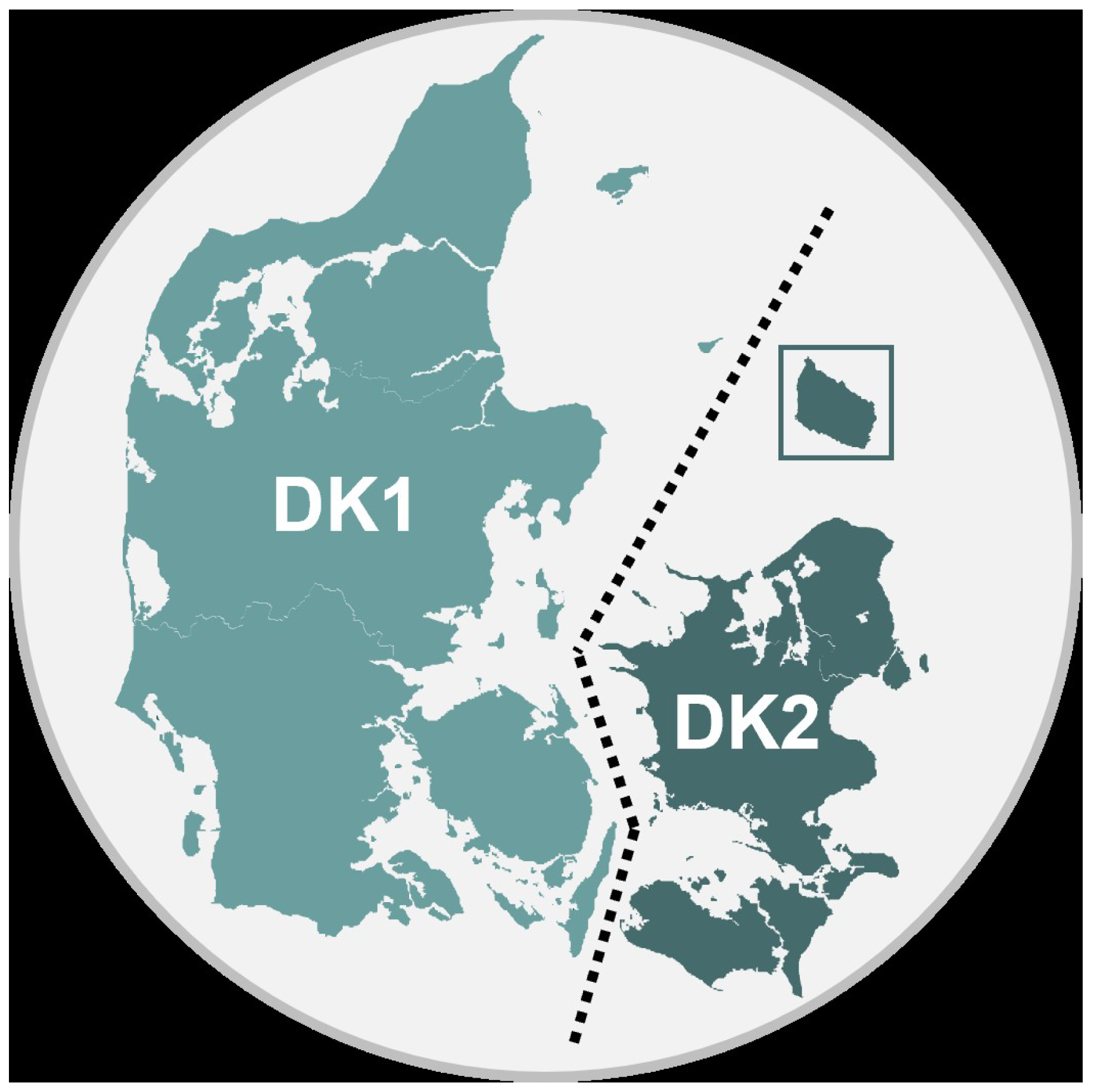
Figure 1. DK1 and DK2 grid regions.
Energies 17 02909 g001
Figure 2. Hourly data for DK1 region.
Energies 17 02909 g002
Figure 3. Data splitting and histograms.
Energies 17 02909 g003
Figure 4. Structure of an LSTM cell [26].
Energies 17 02909 g004
Figure 5. LSTM model results. (a) Mean of the predicted train values vs. the observed train values; (b) Mean of the predicted test values vs. the observed test values; (c) Loss values.
Energies 17 02909 g005
Table 1. Descriptive statistics of intraday and day-ahead prices.
# of ObservationsMinMaxMeanVarianceSkewnessKurtosis
intraday2877−155.68151.6839.89399.96−0.8410.11
day-ahead−83.01121.4639.91328.00−0.985.10
Table 2. Mean scores for the train set and the test set by running 1000 experiments on the LSTM model.
batch size16
epochs50
experiment size1000
time taken by process274 m 29 s
Monte Carlo ScoresTrain ScoresTest Scores
RMSE5.778.41
Scaled RMSE0.020.03
R 2 0.930.81
MAE4.334.64
EVS0.940.82
ME31.9292.38
MdAE3.403.14
Table 3. Performance results of the state-of-the-art models on the test set of the DK1 data.
ModelsRMSEMAEMdAE
XGBoost26.6215.139.06
Random forest24.4014.668.95
LightGBM24.1314.528.11
SVR-RBF19.9810.276.18
KNN14.746.964.23
SARIMA13.056.914.13
CNN 9.49 5.60 3.95
LSTM8.414.643.14
Table 4. Data frame with trading strategies.
Time_StampSolarWindConsIntradayDay
_Ahead
Intraday
_Pred
Profit
_Best
Profit
_Pred
Strategy
_Pred
02019-04-07
01:00:00+2:00
011,952.1240,66038.0937.7138.030.380.38Buy day-ahead,
sell intraday
12019-04-07
02:00:00+2:00
010,686.4039,48037.0137.1337.360.12−0.12Buy day-ahead,
sell intraday
22019-04-07
03:00:00+2:00
09720.2639,21235.3035.5036.240.21−0.21Buy day-ahead,
sell intraday
32019-04-07
04:00:00+2:00
08861.5639,78535.9435.6434.550.30−0.30Short day-ahead,
buy intraday
42019-04-07
05:00:00+2:00
08126.1540,05335.0636.1735.451.111.11Short day-ahead,
buy intraday
Table 5. Summary table of trading strategy results for training and test data sets.
Training Data
(1726 h)
Test Data
(576 h)
Sum of hourly
predicted unit
profits (EUR/MWh)
7042.401418.39
Sum of hourly
best scenario unit
profits (EUR/MWh)
9241.692289.30
Total profit using
production volumes
for predictions (EUR)
≈201,729,893≈35,904,850
Total profit using
production volumes
for best scenario (EUR)
≈243,491,411≈59,353,509
Percentage of strategies
chosen incorrectly (%)
23.4628.35
Disclaimer/Publisher’s Note: The statements, opinions and data contained in all publications are solely those of the individual author(s) and contributor(s) and not of MDPI and/or the editor(s). MDPI and/or the editor(s) disclaim responsibility for any injury to people or property resulting from any ideas, methods, instructions or products referred to in the content.