Article

Combinatorial Component Day-Ahead Load Forecasting through Unanchored Time Series Chain Evaluation

by
Dimitrios Kontogiannis
1,*,
Dimitrios Bargiotas
1,*,
Athanasios Fevgas
1,
Aspassia Daskalopulu
1 and
Lefteri H. Tsoukalas
2
1
Department of Electrical and Computer Engineering, School of Engineering, University of Thessaly, 38334 Volos, Greece
2
Center for Intelligent Energy Systems (CiENS), School of Nuclear Engineering, Purdue University, West Lafayette, IN 47906, USA
*
Authors to whom correspondence should be addressed.
Energies 2024, 17(12), 2844; https://doi.org/10.3390/en17122844
Submission received: 15 May 2024 / Revised: 31 May 2024 / Accepted: 6 June 2024 / Published: 9 June 2024
(This article belongs to the Special Issue Energy, Electrical and Power Engineering 2024)

Abstract

:
Accurate and interpretable short-term load forecasting tasks are essential to the optimal operation of liberalized electricity markets since they contribute to the efficient development of energy trading and demand response strategies as well as the successful integration of renewable energy sources. Consequently, performant day-ahead consumption forecasting models need to capture feature nonlinearities, analyze system dynamics and conserve evolving temporal patterns in order to minimize the impact of noise and adapt to concept drift. Prominent estimators and standalone decomposition-based approaches may not fully address those challenges as they often yield small error rate improvements and omit optimal time series evolution. Therefore, in this work we propose a combinatorial component decomposition method focused on the selection of important renewable generation component sequences extracted from the combined output of seasonal-trend decomposition using locally estimated scatterplot smoothing, singular spectrum analysis and empirical mode decomposition methods. The proposed method was applied on five well-known kernel models in order to evaluate day-ahead consumption forecasts on linear, tree-based and neural network structures. Moreover, for the assessment of pattern conservation, an intuitive metric function, labeled as Weighted Average Unanchored Chain Divergence (WAUCD), based on distance scores and unanchored time series chains is introduced. The results indicated that the application of the combinatorial component method improved the accuracy and the pattern conservation capabilities of most models substantially. In this examination, the long short-term memory (LSTM) and deep neural network (DNN) kernels reduced their mean absolute percentage error by 46.87% and 42.76% respectively and predicted sequences that consistently evolved over 30% closer to the original target in terms of daily and weekly patterns.

1. Introduction

Energy time series analysis and efficient load forecasting tasks contribute towards the optimal operation of liberalized electricity markets since they enhance a plethora of submarket processes and improve the overall grid stability. Accurate load sequence predictions enable dynamic supply and demand balancing through the optimal matching of consumption and generation bids. This results in the optimization of resource allocation processes within the market structure since shortages and excess capacity could be prevented. Furthermore, robust forecasts reinforce market operations through the improvement of decision-making processes, assisting market participants in performing well-informed transactions. Consequently, accurate forecasts form a layer of risk management that enables hedging against electricity price volatility and contribute towards the development of optimal trading strategies that focus on the minimization of investment losses. Additionally, performant load estimation could be beneficial towards the integration of renewable energy sources since the relationship between total demand and renewable generation could be identified and studied extensively in order to obtain a thorough understanding of power system dynamics. The interpretation of energy analytics and the demystification of relationships between load and prominent influential drivers assists in the development of sophisticated demand response approaches since the detailed behavioral analysis of consumption could lead to the detection of insightful patterns and peak demand periods. Moreover, the examination of these patterns could contribute to the avoidance of frequency imbalances, voltage fluctuations as well as extreme events that could compromise grid reliability [1,2]. Therefore, it is evident that load forecasting tasks have a valuable multipurpose role within each submarket and impact the types of market participants differently. In day-ahead markets load forecasting tasks are utilized primarily for demand predictions that target each hour of the next day [3]. On the other side of the spectrum, intraday markets utilize load sequence predictions for near real-time market position adjustments and past prediction updates [4]. Balancing markets utilize load forecasts for the identification of scheduling deviations and capacity markets can ensure the availability of generation capacity through robust forecasting techniques [5]. In terms of market participant impact, accurate load forecasts assist transmission system operators with congestion management through the examination of load patterns and distribution system operators with distributed energy resource integration as well as voltage level management. Additionally, the risk management benefits derived from robust load predictions could enable the emergence of more competitive pricing plans at the retail level [6]. Lastly, consumers are exposed to the indirect effects of load forecasting tasks since consumption adjustments in demand response program participation is heavily influenced by load pattern studies [7].
The overview of the role and importance of load forecasting denotes the accrescent need for robust learning frameworks that capture most of the useful temporal patterns that contribute towards the identification of seasonal effects and dynamic system behaviors. Evidently, the complexity of modern electricity market structures and grid characteristics indicate that the relationships between the target variable of load, commonly referring to electricity consumption, and prominent independent influential factors such as renewable generation are non-linear. These non-linearities typically stem from the intermittent behaviors of the independent variables, since renewable sources do not provide constant electricity generation, as well as underlying weather dependencies, geographical and seasonal variability. Additional non-linearities could be introduced due to storage challenges and technological constraints that may impact the efficiency of renewable generation [8,9]. Consequently, simpler linear architectures that operate under strict assumptions with regards to the structure of the input data often fail to capture meaningful patterns and result in higher prediction error and unsatisfactory generalization capabilities. The negative impact to generalization could be observed clearly on models that produce multi-sequence output based on a target window since the error rate could have an increasing trend for sequences closer to the end of the specified interval [10,11]. The inspection of generalization issues highlights several abnormal error behaviors that enrich the interpretation and evaluation of noisy forecasts, resulting in time series analysis that expands beyond the simple detection of suboptimal predictions. Challenges with regards to error stability could be identified, denoting that substantial oscillations of error metrics across different sequences may not constitute desirable behaviors in the process of interpreting temporal patterns. Furthermore, the random overestimation and underestimation of adjacent data samples within the same sequence could introduce significant complications in pattern recognition processes. It is observed that load time series data often contains consumption patterns that follow long evolutionary paths illustrating the overall behavioral shift in system dynamics. The potential injection of noise in the aftermath of the forecasting process through those subsequent overestimations and underestimations could reveal drastic changes to the evolutionary paths that contribute to the distorted interpretation of patterns and in some extreme scenarios the disqualification of observations due to their classification as outliers. It is worth noting that the injection of noise that leads to this drastic performance deterioration could occur due to a plethora of design choices and data-related challenges. The selection of model parameters that either deviate drastically from the baseline default configuration or do not describe the data structure accurately may result in poor generalization capability. Moreover, the challenges of data drift and concept drift [12,13] could contribute to the eventual undesirable mutation of the evolutionary paths in time series subsequences since changes to the data distribution as the model receives new input observations or difficulties in the mapping between input and target variables during recalibration could result in noisy predictions. Therefore, more complex non-linear architectures coupled with robust preprocessing and evaluation techniques are usually preferred in order to minimize error and interpret patterns accurately.
The scientific fields of machine learning [14] and statistical time series analysis [15] contributed significantly towards the development of robust pipelines featuring preprocessing, forecasting and evaluation techniques that address those important generalization and interpretation issues. Prominent preprocessing methods focusing on these issues include feature selection and time series decomposition techniques. Feature selection methods focus on dataset filtering in order to utilize only the most influential features for prediction. Robust feature selection methods often rely on feature importance metrics derived from the training parameters of kernel estimators such as the Extreme Gradient Boosting model (XGBoost) or from the inspection of feature contribution from permutation-based explainability frameworks such as the Shapley Additive Explanations method (SHAP) [16]. On the other side of the spectrum, time series decomposition methods focus on the isolation of data patterns, the separation of noise from the original sequence and the efficient handling of non-stationarity. Commonly used methodologies such as the Seasonal-Trend decomposition using Locally estimated scatterplot smoothing (STL) and Singular Spectrum Analysis (SSA) focus on the derivation of seasonal, trend and residual components in order to form fine-grained representations of the input. Furthermore, data-adaptive multiresolution decomposition methods such as Empirical Mode Decomposition (EMD) target the efficient representation of intrinsic oscillations and the inspection of local behaviors within time series sequences in the time-frequency space without forming any a priori assumptions [17]. These preprocessing methods are typically connected to several standalone and combinatorial forecasting structures for the robust estimation of time series sequences. Linear models such as Linear Regression (LR) [18] and the regularized variants of Ridge [19] and Lasso Regression [20] are often developed to derive a simple and interpretable baseline that denotes the impact of observed nonlinearities through performance deterioration. Furthermore, tree-based regressors such as Random Forest and XGBoost algorithms provide computationally efficient, parallelizable and flexible solutions to the prediction of nonlinear load time series and are often utilized as standalone or hybrid kernels in forecasting frameworks [21,22]. Lastly, neural network models such as the Multi-Layer Perceptron (MLP) and the Long Short-Term Memory network (LSTM) are black-box approaches that enable adaptive and accurate approximation of complex non-linear functions and exhibit improved resilience towards missing values and outliers [23,24,25,26,27,28]. It is worth noting that advances in neural network research led to the integration of attention mechanisms such as self-attention and multi-head attention [29]. These attention mechanisms enhanced the interpretability of complex neural network architectures and contributed towards the development of models that focus on the most important parts of the data in order to express non-linear relationships. The performance evaluation of those forecasting pipelines is heavily dependent on the study and visualization of error metrics. Error functions such as Mean Absolute Error (MAE), Mean Absolute Percentage Error (MAPE), Mean Squared Error (MSE) and Root Mean Squared Error (RMSE) constitute insightful metrics that study different characteristics of the deviation between the actual and predicted values. The inspection and visualization of each standalone error metric enables robust model comparisons. Moreover, the co-inspection of those error metric values and graphs assists in the interpretation of large error impact [30,31].
Several recent research projects examined the application of feature extraction and decomposition techniques on statistical and machine learning models for load forecasting tasks and proposed interesting methodologies. Dong et al. [32] presented a hybrid regressive neural network model that utilizes EMD and genetic algorithm optimization in order to extract knowledge from the nonlinearities of load observations. The proposed model was evaluated through the point forecasting metrics of absolute and relative error as well as the comprehensive error metrics of MAE, RMSE and MAPE denoting high fitting ability and error stability. Qiuyu et al. [33] presented a case study highlighting the effectiveness of STL decomposition on Support Vector Regression (SVR) and artificial neural network models, illustrating significant decrease of the average MAPE and the error of maximum load. Cheng et al. [34] developed a Deep Neural Network model (DNN) for very short-term load forecasts based on correlation and principal component analysis for feature selection and EMD for pattern extraction. The proposed methodology outperformed deep neural network variants utilizing the original dataset and wavelet decomposition. Bedi and Toshniwal [35] introduced a technique utilizing Variational Mode Decomposition (VMD), an autoencoder and an LSTM network for average and peak demand predictions evaluated through MAPE graphs and RMSE for the training and test set. This complex architecture outperformed state-of-the-art demand prediction models denoting the potency of decomposition-based hybrid approaches at the cost of convergence time. Safari et al. [36] examined the performance issues and limitations of EMD as a standalone decomposition technique in load and renewable time series forecasting, highlighting the need for methods that address the impact of incomplete cycles near the edges of time series sequences. Langenberg [37] studied the performance of decomposition-ensemble algorithms and concluded that the multiple STL variant coupled with the double seasonal additive Holt-Winter’s method and multivariate adaptive regression splines outperformed hybrid models using neural network and linear regression structures. Taheri et al. [38] decomposed the target load variables through EMD and utilized an ensemble consisting of LSTM members to derive the aggregated predictions. The proposed model yielded lower error metrics when compared to standalone LSTM, LR and XGBoost approaches, outlining the significance of time-frequency decomposition methods in order to address load uncertainties and non-linearities. Stratigakos et al. [39] applied SSA on MLP and LSTM models for multiple sequence predictions and observed that in terms of MAPE, the LSTM combination outperformed the standalone baseline models as well as the MLP-SSA combination. Moreover, Pham et al. [40] combined SSA with a backpropagation neural network and an LSTM network and through an electrical load demand case study reinforced the observation that the SSA-LSTM combination performs better than other decomposition-kernel model variants. Zhang et al. [41] coupled VMD with a stacked ensemble model for short-term load predictions utilizing XGBoost, LSTM, SVR and k-nearest neighbor (KNN) kernels. This method yielded significantly improved performance over the standalone kernels that did not apply decomposition. Liu et al. [42] forecasted user energy consumption through noise-assisted complete ensemble EMD and LSTM networks. This project showed improved performance in terms of RMSE and MAE when compared to standalone LSTM and recurrent neural networks, illustrating the derivation of stable components that reflect periodicity and trends. Sun et al. [43] utilized VMD and kernel extreme learning machines in order to decompose the target variable of demand-side load and subsequently predict each sub-modal component, resulting in a methodology that achieves lower error metrics when tested on different types of electricity consumption. Duong et al. [44] highlighted the RMSE and MAPE improvement of a combinatorial STL-LSTM method when compared to standalone artificial neural networks such as the LSTM structure and the combination of convolutional neural networks with LSTM for peak load forecasts. Huang et al. [45] proposed a two-stage short-term forecasting model which utilized SSA and VMD for decomposition, an LSTM for high-frequency component prediction and a multiple LR model for low-frequency component prediction. The experimental evaluation of this method illustrated increased predictive potency and stability in terms of RMSE, MAE and MAPE values at the cost of computing time. Wood et al. [46] utilized EMD for feature engineering, k-means clustering for outlier detection and LSTM networks for day-ahead load prediction in a forecasting framework that often outperforms the naïve moving average method and results in more robust forecasts. Sohrabbeig et al. [47] acknowledged the presence of multi-seasonal components in time series datasets and developed a multi-seasonal trend decomposition model for the separate forecasting of trend, seasonal and residual load components through linear layers. The results of this work demonstrated the superiority of this method in terms of MSE and MAE when compared to transformers and several linear benchmarks. Yin et al. [48] utilized EMD and fluctuation analysis in order to detect different types of long-range intrinsic mode functions and coupled with the derivation of the linear and periodic components, extract the aggregated predictions through an LSTM structure. The proposed model yielded impressive performance on high resolution load data, outperforming the standalone LSTM structure as well as combinatorial LSTM structures utilizing the STL and SSA decomposition techniques.
Evidently, the examination of the literature surrounding the application of decomposition methods in load forecasting tasks highlighted significant performance improvements when these approaches are applied to the input for the construction of descriptive and robust feature sets as well as the output for the aggregation of load component forecasts. Additionally, LSTM networks often process the component structure more efficiently in those approaches, resulting in more stable predictions. However, it is observed that recent research studies often overlook two important areas with regards to the application and evaluation of decomposition methods.
Firstly, most component-based feature sets utilized for prediction tasks are extracted from standalone decomposition methods. Clearly, there are several pitfalls that stem from the sole reliance on standalone decomposition approaches and recent research may not address them sufficiently. Decomposition methods differ in terms of their pattern sensitivity and while a standalone method may yield improved performance, the set of patterns discovered and captured by two different methods does not exhibit a full overlap. As a result, the selection of a standalone methodology may lead to the omission of some important patterns that could yield lower error metrics and more stable predictions. In more extreme scenarios, the dependence on standalone decomposition approaches could result in performance deterioration due to the incompatibility between the assumptions of the model and the underlying structure of the data. Consequently, the oversimplified or misinterpreted representation of input or target features across more diverse datasets may not address temporal data intricacies effectively. This effect could be considered as model selection bias that could negatively impact forecasting performance since it would result in limited adaptability and robustness.
Secondly, the evaluation of decomposition-based models in recent studies focuses on the visualization of case-specific intervals, the inspection of prominent error metrics as well as the examination of interpretability functions in order to study the impact of errors, derive conclusions on model stability across different sequences and quantify the compatibility between the forecasted target and the component-based structure. While these evaluation approaches may be considered robust in terms of error analysis standards, they do not provide direct information regarding the impact of the forecasting methodology on the conservation of the intended pattern evolution across multiple sequences. Therefore, while the values of error metrics could indicate predictions that are close to the actual sequences, slight overestimations and underestimations may result in significant temporal pattern distortion, altering the behavior of the forecasted series. The consequences of this effect become apparent during the examination of the unconditionally longest time series chains within load sequences. Since these chains denote the longest evolutionary paths within a sequence, they are significant in the study of load time series dynamics and the underlying temporal structure. As a result, the temporal distortions could lead to forecasted load time series that evolve in completely different ways when compared to the actual load. This deviation in evolutionary paths could easily remain undetected during model evaluation since the starting points of long time series chains may differ drastically from the endpoints. Omitting the goal of evolution preservation could lead to interpretability issues and performance deterioration as more significant deviations through time could fail to provide a descriptive representation of the original target series. Concludingly, the development of performant combinatorial decomposition methods and the conservation of evolutionary time series paths constitute important research areas that are not sufficiently explored.
In this study, we focused on the development of a combinatorial decomposition-based methodology for day-ahead load forecasting. Additionally, we examined the conservation of the longest evolutionary paths after the forecasting process through a novel evaluation method. The proposed methodology combined STL, SSA and EMD in order to extract time and frequency domain components that capture seasonality, trend and residual patterns from influential renewable generation features as well as lagged load variables. The most important components derived from an XGBoost scoring method were utilized for the prediction of 24-hourly load sequences through five different kernel models. The set of kernel models consist of different types of prominent estimators including a linear regressor, an XGBoost model, an MLP, an LSTM and an attention LSTM variant utilizing self-attention. The model performance was evaluated through a case study featuring five years of electricity consumption, solar and wind generation observations for the Greek power system. The error analysis consisted of prominent error metrics including MAE, MAPE, MSE and RMSE. Additionally, the evaluation of evolution conservation considers the data mining primitive of time series chains and through the extraction of the unanchored chains for each hourly sequence, the weighted average unanchored chain closeness is calculated based on the distance between actual and predicted subsequences within each chain for daily and weekly patterns. This calculation considers the Euclidean distance [49] in order to derive a more pessimistic closeness estimate and Dynamic Time Warping (DTW) [50] in order to derive a more optimistic estimate due to the minimization of temporal distortions within each subsequence.
The contribution of this research work is threefold. Firstly, the development of the combinatorial decomposition method explores the effects of different data representations at the preprocessing stage and highlights important behaviors of prominent estimation structures in the day-ahead load forecasting task. As a result, this approach provides insights towards the design and development of sophisticated decomposition pipelines that involve processes focusing on influential component-based fusion. This combination of methodologies addresses the simultaneous local and global decomposition in the time and frequency domains while utilizing information extracted from paradigms that consider different levels of data-specific assumptions. The novelty of this approach is evident due to the lack of versatile combinatorial methods in recent literature. The introduction of performant component-based methods that blend load decomposition techniques directly addresses most pitfalls in standalone component-based modeling since it exposes estimators to a wider spectrum of nonlinear patterns and addresses the unexplored performance benefits of this approach under an interpretable importance-based framework. Additionally, the study of different kernel estimator types provides a holistic view of the predictive potency that those methods could enable when utilized in frameworks that handle non-linearities at different levels of granularity.
Secondly, the examination of model performance beyond the typical error analysis, reinforces the value of this method and introduces a novel evaluation approach based on the intuitive concept of time series chain similarity. Since most studies rely on a specific set of traditional error metrics, the effects of temporal drift within the decomposed sequence structure and the evolutionary behavior of the target are often omitted. The distance-based scores obtained by the proposed approach directly address the uncertainty in the quantification of evolution conservation and the inspection of temporal distortions in the longest chains of daily and weekly subsequences. Furthermore, the proposed evaluation method offers increased flexibility since the type of distance kernel, the length of the studied subsequences and the length of the time series could be configured. The adjustment and future enhancement of those parameters could enable the examination of different types of evolutionary paths, boosting the adaptability and interpretability of this method.
Thirdly, this work contributes to the design and development of a combinatorial approach that could yield more accurate and stable short-term forecasts across several types of estimators, assisting in the efficient discovery of relationships between renewable generation and electricity consumption and subsequently optimizing several energy market processes that focus on optimal renewable integration. The inclusion of the proposed evaluation method provides more intuitive tools at the disposal of developers and analysts in the energy sector, highlighting processes that focus on important time series data mining primitives. Therefore, it is evident that this research project could enable field-specific advancements through the improvement of component-based forecasting methods and performance evaluation metrics. Additionally, this project could influence modern market applications towards increased future energy market efficiency.
In Section 2, we analyze methodologies that contributed towards the development and evaluation of the proposed combinatorial method referencing, decomposition methods, kernel estimators and time series chains concepts.. The following subsections include the dataset overview, decomposition and estimator model configurations as well as important implementation characteristics. Furthermore, the performance metrics utilized in the evaluation of this approach are analyzed, presenting an overview of traditional error metrics and introducing the pattern conservation metric. In Section 3, we present the results derived from our experiments and evaluate the proposed forecasting structure through a detailed comparison with baseline models utilizing different estimator types. In Section 4 we discuss about the overall performance of the model while addressing important advantages, disadvantages, development challenges and future research directions. In Section 5, we provide a concise overview of concluding comments on our research findings and we summarize our thoughts on the importance of this research contribution.

2. Materials and Methods

2.1. Time Series Decomposition Methods

Time series decomposition methods constitute powerful feature processing tools since they enable pattern extraction in the time and frequency domains. The set of temporal components extracted from those techniques typically includes trend, seasonal and residual sequences, each representing a different type of behavior for the original time series variable. Trend sequences aim to describe the secular variation in time series variables and could indicate an increasing or decreasing direction of sequence values. The analysis of trend could also uncover cyclical behaviors associated with recurrent aperiodic variations that depend on the time series structure. Seasonal sequences represent the variations that occur at regular time intervals due to the dependence of the original variable to time-domain characteristics and exogenous factors such as weather variables. Residual sequences describe irregular variations in time series that often stem from the randomness introduced by noise and other data anomalies. Prominent decomposition methods focusing on the derivation of temporal components often consider the structure of an additive or multiplicative model based on the relationship between the variations around the trend component and the level of the time series. The additive model considers the addition of the trend, seasonal and residual component for the reconstruction of the original sequence while the multiplicative model considers the product of those components as described in the following formulae, where y t represents the target sequence at timestep t and T t , S t , and R t represent the trend, seasonal and residual component respectively for the same timestep:
y t = T t + S t + R t
y t = T t × S t × R t
It is worth mentioning that the temporal components may not be linear since the structure of the time series could indicate non-linearities through more complex trend patterns, non-linear variations in the amplitude of seasonal effects or the intrinsic irregularities in the residual sequence. On the other side of the spectrum, in the frequency domain, the oscillatory behaviors are commonly represented as a set of sinusoidal functions that express the frequency content of the series or as a set of intrinsic mode functions that capture different oscillatory patterns and through their envelope properties define boundaries where those behaviors occur in dominant frequencies. The decomposition methods offer increased flexibility and adaptability since they can be applied on the input as well as on the target output, resulting in enhanced preprocessing approaches. The decomposition of input variables alters the dimensions of the dataset in order to explicitly define sequences that represent important patterns. In this context, the learning process becomes easier as the unraveled data exposes the structural characteristics clearly and could contribute towards improved estimator accuracy. The decomposition of the target output enables distributed forecasting through advanced hybrid and ensemble methods that use multiple different estimators for the prediction of each component [51]. Consequently, these approaches could yield performance benefits due to the increase of tunable model parameters and clarity of target representation but they could also become more computationally expensive. For the purposes of this study, we utilize the combination of three prominent decomposition methods to examine the performance benefits that stem from the selection of the most influential components with regards to well-known standalone estimators. The following subsections present a concise overview of the STL, SSA and EMD methodologies that were utilized for component extraction.

2.1.1. Seasonal-Trend Decomposition using Locally Estimated Scatterplot Smoothing

The STL decomposition method combines local regression with an iterative process in order to derive the seasonal, trend and residual components from a given time series. This iterative process consists of two recursive methods, forming an inner loop and an outer loop. The inner loop performs component smoothing through regression curves and derives updated representations of the seasonal and trend sequences. Polynomials fit to local subsets of data within each component and the contribution of each data point to that local regression process is calculated through neighborhood weights that reflect the distance of each data point to the target observation. The outer loop derives the residual sequence and calculates robustness weights that reflect the impact of deviations on the trend and seasonal components. Those weights are initialized to the value of 1 and express the reliability of an observation relative to the others. In the smoothing processes, the integration of robustness weights is achieved through their multiplication with neighborhood weights.
Furthermore, the STL algorithm is sufficiently flexible since various types of seasonal behaviors and trends could be modeled through the control of parameters such as the seasonal and trend-cycle window that regulate the rate at which those components change. The convergence of this method commonly depends on threshold methods that examine the difference between consecutive estimates of component sequences as well as the number of iterations for the outer and inner loops. This method is robust to outliers since the impact of noise mainly affects the residual component [52].

2.1.2. Singular Spectrum Analysis

The SSA decomposition method is a nonparametric spectral estimation approach that focuses on the derivation of seasonal, trend and residual components through lag embedding and the inspection of eigenvalues and eigenvectors. In the first step of this approach, lag embedding occurs through the transformation of the time series into a Hankel trajectory matrix Y where each column represents a lagged time series segment in the multidimensional space. Following this step, Singular Value Decomposition (SVD) is applied to this matrix in order to derive the diagonal matrix Λ containing singular values λ i and the orthogonal eigenvector matrices P and P T containing left-singular vectors l i and right-singular vectors r i respectively. This decomposition is expressed by the following formula, where the superscript T indicates the transpose of the respective matrices:
Y Y T = P Λ P T
Subsequently, the trend, seasonal and residual component sequences are derived from the inspection of eigentriples ( l i , λ i , r i ) . The observation of large and slowly decaying singular values within the eigentriples may indicate the existence of a trend or seasonal pattern. Smooth and gradual variations of left-singular vectors as well as gradual and systematic patterns on right-singular vectors could contribute towards the extraction of the trend sequence. Periodic and repeating behaviors on left and right-singular vectors could contribute towards the extraction of the seasonal sequence. The remaining eigentriples that do not exhibit any of the previously discussed characteristics could assist in the identification of the residual sequence. Consequently, each component could be extracted from a reconstruction process involving sums of eigentriples that share those characteristics. The following formula denotes the calculation of T t , S t , and R t at timestep t after the discovery of n relevant eigentriples:
T t , S t , R t = i = 1 n λ i l i r i T
In terms of user-defined parameters, SSA implementations commonly feature the size of the sliding window that determines the length of the subseries used for the creation of the trajectory matrix and the number of groups that denotes the total number of extracted components [53].

2.1.3. Empirical Mode Decomposition

The EMD method is a data-driven and adaptive approach that focuses on the intuitive representation of oscillatory time series behaviors in order to study sequence dynamics. This methodology, unlike the Fourier Transform, aims to isolate temporally adaptive basis functions and derive frequency dynamics directly from them, instead of attempting to interpret the complex combination of multiple harmonics. Consequently, this approach presents an alternative perspective where sequence dynamics such as instantaneous amplitude, frequency and phase are not obtained from static basis functions but from adaptive intrinsic mode functions (IMF). The IMFs are functions obtained from the sifting algorithm in the time domain and share several similar characteristics such as local symmetry around zero and equality between their extrema and zero-crossings. The sifting algorithm is an iterative approach that extracts oscillatory time series components, starting from the identification of the fastest dynamics and proceeding until a non-oscillatory trend remains. At the first step of this algorithm, the local extrema of the time series are identified. Following this step, upper and lower envelopes are formed by connecting the extrema through cubic spline interpolation. The first IMF is extracted by subtracting the mean of the envelopes from the sequence. Subsequent iterations consider the last extracted IMF as the source sequence and repeat this process until the last non-oscillatory component is identified.
The set of prominent parameters utilized in EMD implementations includes the number of IMFs, the interpolation method and the stopping criterion. The selection of the number of IMFs is typically data-specific and constitutes an integral part in the design of load forecasting modes involving EMD since the extracted oscillatory components need to express sufficiently fast and distinct dynamics in order to provide meaningful information during the learning process. The interpolation method mainly influences the smoothness of the extracted IMFs and as it was previously mentioned, cubic spline interpolation is commonly preferred in the sifting algorithm. Lastly, the stopping criterion could be defined as the threshold denoting that the residual IMF is non-oscillatory or as a maximum number of iterations that is selected due to computational constraints [54].

2.2. Forecasting Models

2.2.1. Linear Regression

Linear regression constitutes one of the simpler machine learning approaches for load forecasting models since it focuses on the search for the line of best fit. The goal is to find the linear combination of independent input variables that minimizes the prediction error for each of the target sequences. Linear regressors in their general form could include an autoregressive component, derived from the selection of target time series lags as input variables, as well as an exogenous component stemming from a plethora of influential factors included in the dataset. Following this general form, each target sequence y can be expressed as the linear combination of input sequences x i that contribute to the model at a level described by their weights w i . These weights, also known as regression coefficients, could be interpreted as slopes in the context of line fitting. The following formula presents this combination given the initial weight w 0 denoting the line intercept and the error term ε   derived from the sum of squared differences between actual and predicted values:
y = w 0 + i = 1 k w i x i + ε
This type of estimator could derive the coefficients analytically through the ordinary least squares (OLS) method or iteratively through stochastic gradient descent optimization in order to minimize the error term. After this minimization process and the discovery of the line that best fits the data, the influence of input features could easily be interpreted through the examination of the weight magnitudes and signs as well as several statistical tests that focus of the quantification of variable significance in load predictions. The inspection of the absolute weight values could lead to the extraction of information regarding the impact of input variables. The sign of regression coefficients could assist in the identification of the direction in the relationship between the input and target variables since positive coefficients could indicate value changes towards the same direction and negative coefficients could denote value changes towards the opposite direction. Therefore, linear regression is often utilized in load forecasting tasks due to this profound ease of implementation and interpretation despite encountering several challenges such as the proneness to overfitting and the reliance to the restrictive assumptions of linearity, homoscedasticity, weak exogeneity, imperfect multicollinearity and statistical error independence [55]. For the purposes of this study, the OLS linear regression is utilized as a naïve linear kernel for the estimation of baseline and combinatorial component performance in order to challenge the impact of the previous assumptions and study the behavior of the model when several components that express non-linearities are present in the input.

2.2.2. Extreme Gradient Boosting

The XGBoost algorithm is a performant regression method in load forecasting that relies on the structure of decision trees and utilizes ensemble learning principles in order to derive accurate and robust time series predictions. According to this methodology, a series of weak decision tree learners are trained sequentially, with each subsequent learner focusing on the correction of errors made by previous estimators. The training process aims to modify several parameters in order to minimize an objective function consisting of the loss function and the regularization term. The loss function l measures model performance with regards to the deviation of the predicted values y i ^ when compared to the observations y i in the training set. The regularization term Ω is formed with regards to each decision tree member f k and penalizes the complexity of the model to prevent overfitting. The objective function L ( φ ) of the XGBoost method is expressed by the following formula:
L ( φ ) = i l ( y i ^ , y i ) + k Ω ( f k )
Decision tree members are built using a breadth-first approach and the best split points are identified through the evaluation of candidate splits with regards to maximizing the improvement of the objective function. Prominent model parameters considered during the training of XGBoost regressors include the learning rate that modifies the contribution of tree-based learners, the maximum tree depth, the minimum split loss, sampling percentages for input features as well as regularization parameters and structural parameters influencing the data needed for the creation of a new node. The boosting process involves the repeated computation of loss function gradients, weak learner fitting, prediction updates and application of regularization. The final predictions are obtained through the aggregation of learner outputs when the boosting process meets the specified convergence criteria such as the maximum number of boosting rounds or a loss function threshold. The XGBoost methodology provides a scalable and sparsity-aware solution that is resilient to outliers and sufficiently interpretable due to the underlying tree structure that forms compact decision rules [56]. In this study, the role of XGBoost is twofold. Firstly, XGBoost is utilized in the feature selection process for the designation of the most influential input components. Secondly, this methodology is selected as one of the studied day-ahead load estimator kernels to examine the performance of a prominent tree-based regressor in the baseline as well as the combinatorial component-based scenario.

2.2.3. Multi-Layer Perceptron

The multi-layer perceptron extends the perceptron learning algorithm in order to form the class of feed forward artificial neural networks that share several characteristics with regards to the model structure and the training procedure. Multi-layer perceptron estimators rely on the computation units called neurons, that are organized following a layer structure. This structure typically contains the input layer, several hidden layers and the output layer. The role of the input layer is to receive the input features and pass them to the hidden layers. Subsequently, the hidden layers focus on learning and extracting feature from the input data, resulting in a computational path that connects the input to the output. The output layer processes the information made available at the after the last hidden layer and the predictions for the target sequences at each neuron. The flow of information throughout this structure is regulated by weight matrices and bias vectors. Additionally, the output of each neuron within a layer is determined by an activation function. The weights in the MLP structure denote the strength of connections between neurons in different layers and represent the importance of an input feature from one neuron to the output of another. Furthermore, the bias vectors indicate the shift in the neuron outputs that influences their activation by providing additional freedom in the modeling of more complex relationships. Activation functions produce the output of each neuron and introduce non-linearities that enhance the learning capabilities of the model. The main objective of the MLP regressor in load forecasting tasks is to approximate the function that describes the relationship between the input and the target sequences. This function approximation process aims to minimize error functions expressing the difference between actual and predicted values.
For the thorough understanding of the forward information flow in MLP we consider an example network featuring one hidden layer for the approximation of the function f :   R D   R L , where D refers to the dimensions of input vector x , and L refers to the dimensions of the output vector f x . Following the matrix notation, the information flow from the input layer to the first hidden layer introduces the weight matrix W 1 that is multiplied with the input vector and the bias vector b 1 that shifts the result of this multiplication. The derived term combining weights and biases passes through the activation function s , producing the output of the hidden layer. Symmetrically, this process continues for the expansion of the approximated function in order to express the information flow from the hidden layer to the output layer through the introduction of weight matrix W 2 , bias vector b 2 and activation function G . Consequently, the function expressing the forward information flow for this example structure is defined by the following formula:
f x = G b 2 + W 2 s b 1 + W 1 x
An overview of the MLP structure with one hidden layer is presented in Figure 1 for the approximation of m output sequences given n inputs, where each symbol corresponds to the symbols of Formula (7) [57,58].
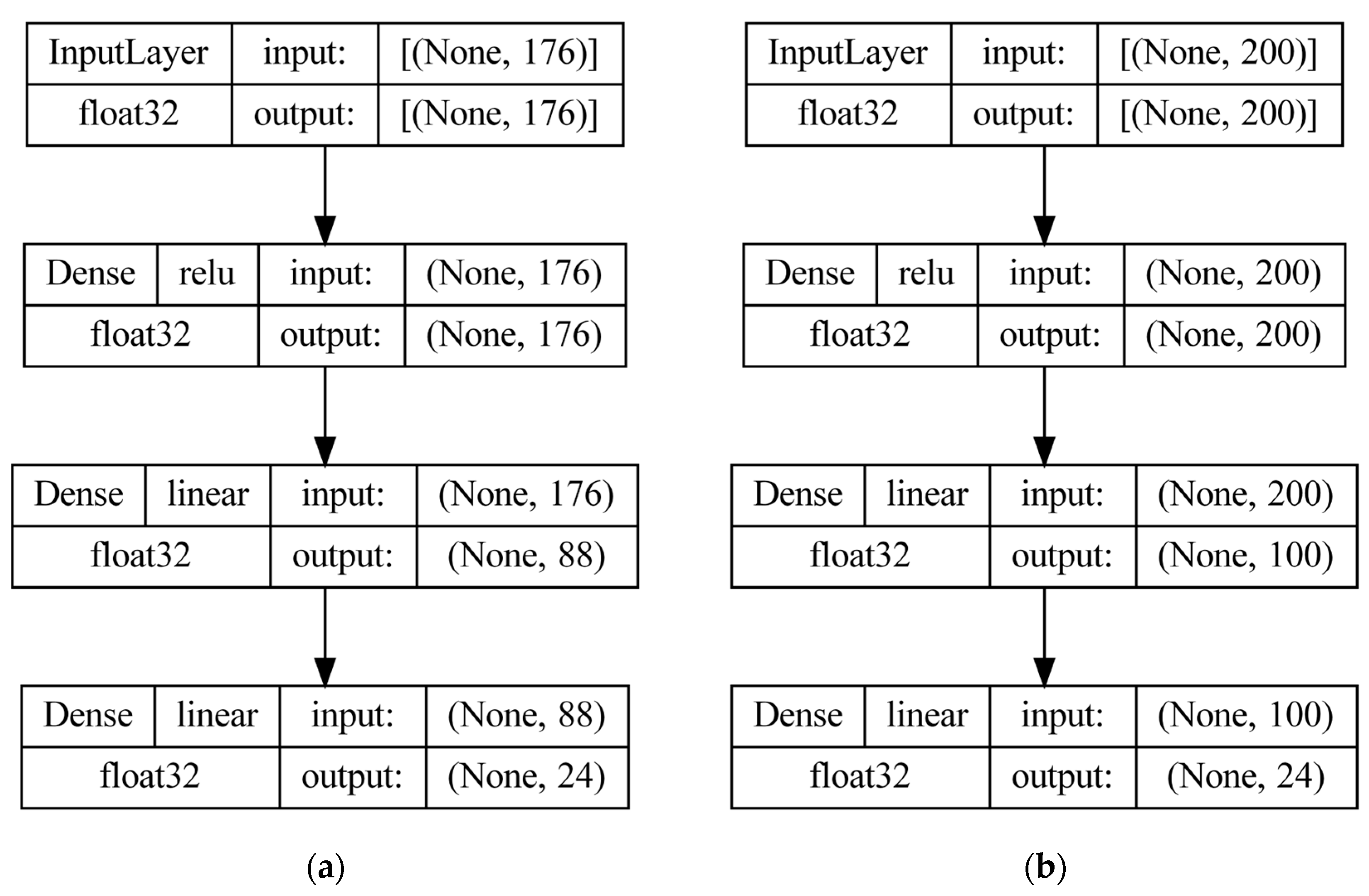
The training of MLP regressors commonly relies on the back propagation algorithm and the gradient descent process in order to adjust weight and bias values through several data passes until convergence is achieved. Convergence in the context of MLP training is interpreted through the examination of the error function as well as the maximum number of data passes. Therefore, convergence could be observed when the values of the error function do not improve significantly through subsequent data passes. Alternatively, the output of the model at the maximum number of iterations could be accepted for performance evaluation due to computational constraints. Commonly used hyperparameters for the design of this model include the number of layers as well as the number of neurons per layer, the type of activation function and the learning rate of the optimizer [59]. In this study, an MLP architecture with two hidden layers and structural hyperparameters proportional to the input is considered as a baseline and combinatorial component kernel in order to study the behavioral shift in the forecasting process of deep artificial neural networks when influential sequence components are considered.

2.2.4. Long Short-Term Memory Networks

Long short-term memory networks belong to the class of recurrent neural networks (RNN) and focus on the identification of long-term data dependencies, rendering them useful for sequence modeling tasks. The LSTM architectures improve upon the RNN baseline since they address the vanishing gradient problem that often impacts RNN generalization capabilities when attempting to extract knowledge from long-term data dependencies. The structure of LSTM networks consists of processing units knows as LSTM cells. Each cell has its own state that expresses the global memory of the network through time, allowing the model to capture and preserve long-term dependencies. Additionally, each cell contains a hidden state that captures short-term information about the sequence. The current cell state of an LSTM cell c t is influenced by the cell state of the previous time step c t 1 as well as the information that could potentially be included at the current timestep. The current hidden state of the cell h t is directly influenced by the derivation of the current cell state. This relationship between the cell state and the hidden state is expressed computationally through several data modifications that occur in each cell. A set of gates within each cell operates in order to apply those adjustments and form the current cell and hidden state. Each cell contains an input gate, a forget gate and an output gate. The input gate at timestep t , denoted as i t utilizes the current input x t and the previous hidden state of the cell h t 1 in order to determine which values will be updated and stored in the current cell state. The output gate at timestep t , denoted as o t , determines which information will be transferred to the output of the cell, influencing the current hidden state through the processing of the current input and the previous hidden state. The following formulae express the information processing of the input and output gates, where w i and w o are the respective weights of those gates, b i and b o are the biases, and σ is the sigmoid function:
i t = σ w i h t 1 , x t + b i
o t = σ w o h t 1 , x t + b o
The forget gate at timestep t , denoted as f t , selects the information that will be removed from the cell state through the examination of current input and the previous cell state. Given the definition of w f weights and b f biases, the forget gate is expressed as:
f t = σ w f h t 1 , x t + b f
The information that could potentially be stored to the current cell state define the candidate sequence d t , derived from the previous hidden state and the current input through the subsequent definition of weights w d and biases b d . Therefore, the candidate sequence and the derived cell state and hidden state are expressed with regards to the application of the previous gates through the following formulae:
d t = t a n h w d h t 1 , x t + b d
c t = f t c t 1 + i t d t
h t = o t t a n h c t
Figure 2 presents a high-level overview of connected LSTM cells for the derivation of the hidden LSTM states and the updates to the current LSTM state at each timestep.
The training of LSTM networks commonly involves the back propagation algorithm through time and the gradient descent method for error minimization. The performance of this type of neural network could depend on several structural parameters such as the number of cells and the number of hidden LSTM layers. Additionally, the selection of activation function, the introduction of dropout and the control of weight initialization, weight decay rate, learning rate and momentum strategies could impact the final forecasting output [60].
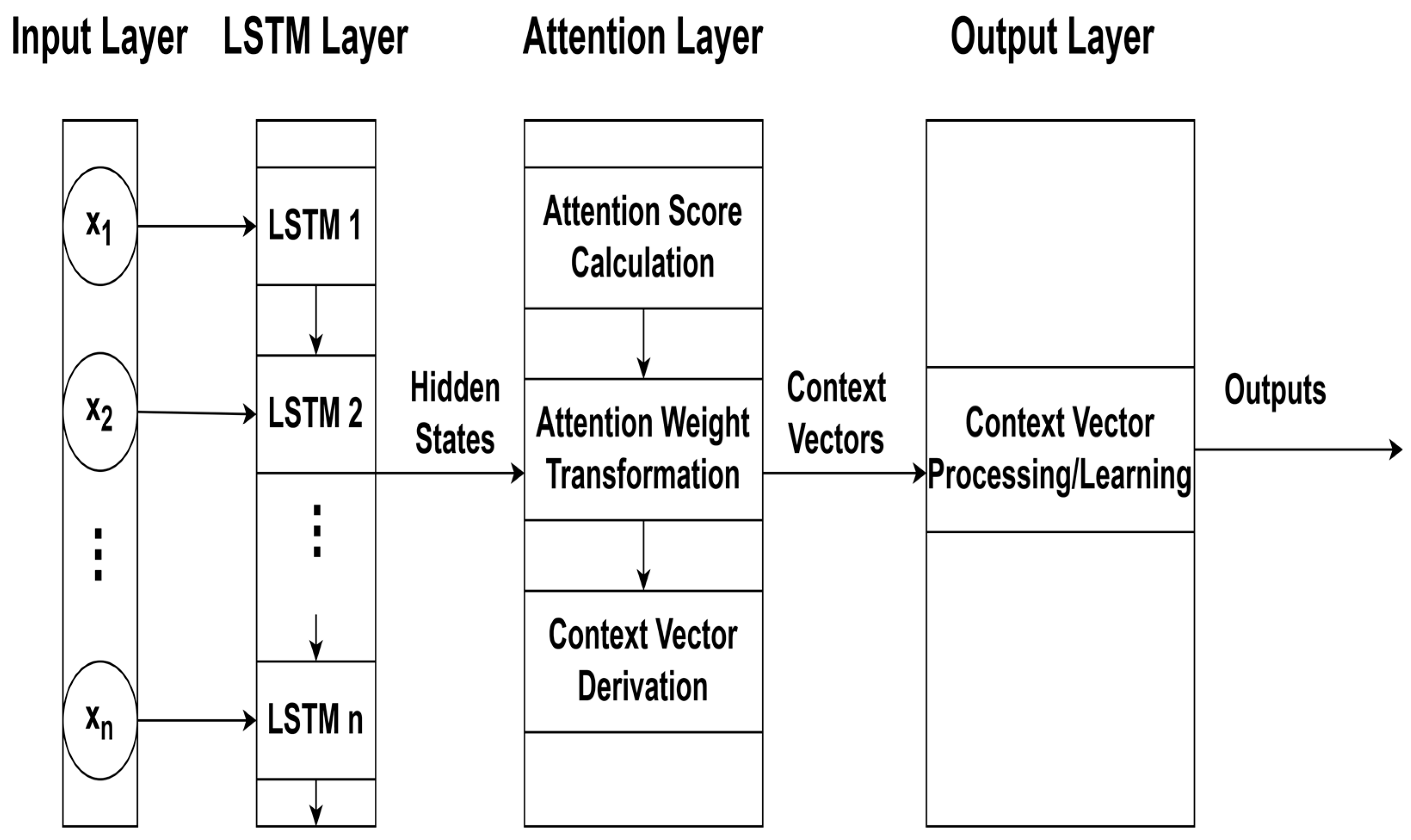
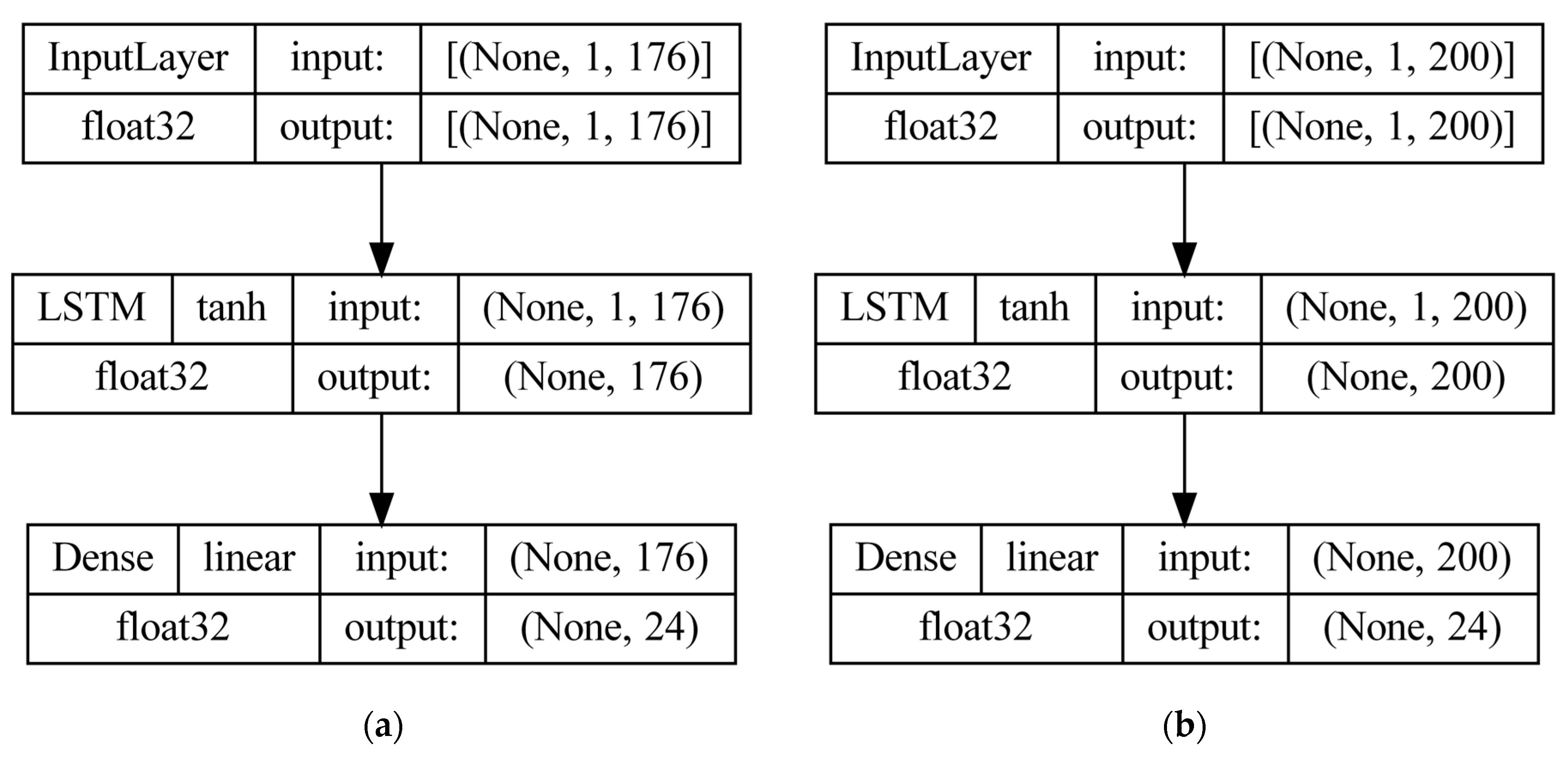
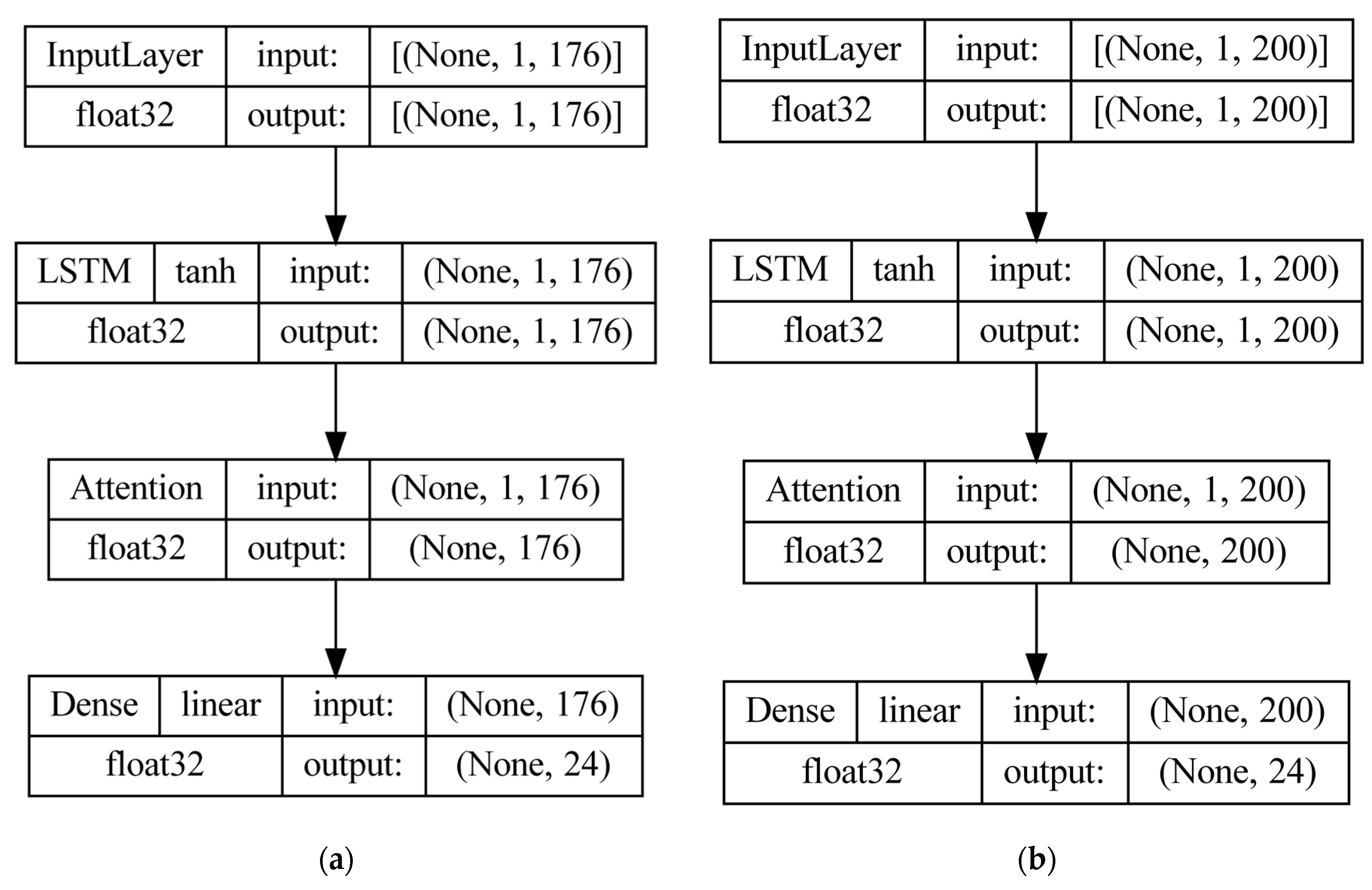
It is worth mentioning that given a specific LSTM configuration, attention mechanisms could be applied to the output sequences of LSTM layers in order to enable the model to selectively focus on different parts of the input sequence and dynamically adjust the importance of time series observations. The integration of attention mechanisms involves the definition of attention layers that utilize predefined input sequences representing network states or time series embeddings as the main processing sources. Following the definition of the input, attention scores are typically derived through computations applied on the trainable parameters of the layer involving scoring or alignment functions that assist in the quantification of relevance or importance of each input element with regards to a specific context. The extracted attention scores are transformed into a probability distribution that is suitable for weighting the input sequence through the softmax function, which ensures that the sum of the outputs equals to one, deriving attention weights. The weighted sum of input sequence elements using attention weights produces the context vectors that could be utilized as standalone sequences or as complementary features in subsequent processing steps for the generation of robust and interpretable predictions. The inclusion of attention layers in LSTM architectures could simplify the processed time series structures and provide memory-efficient and context-aware alternatives that address the challenge of dimensionality through the utilization of context vectors [61]. Consequently, in this study two LSTM variants are examined. The first contains a hidden LSTM layer and the second enhances that structure through the inclusion of an attention layer for the examination of the combinatorial component performance based on extracted context vectors. Figure 3 illustrates the learning task for n inputs based on context vectors through the integration of an attention strategy in a single layer LSTM structure.

2.3. Time Series Chains

The evaluation of load forecasting model performance is prominently expressed through error metrics that measure the deviation between actual and predicted values. These methods could be utilized for the robust point-by-point monitoring of convergence, the impact of large prediction errors within the output sequences or the error stability across different time series lags. These methodologies emphasize the inspection of point observations during the training stages as well as after the derivation of the complete output sequences. Point observations offer high granularity in error analysis but they are limited in scope since information about the evolutionary paths within sequences and the comparison between drifting patterns is not explicit and interpretable. As a result, the consideration of subsequence analysis and the inspection of time series chains is crucial for the thorough understanding of time series evolution and pattern conservation.
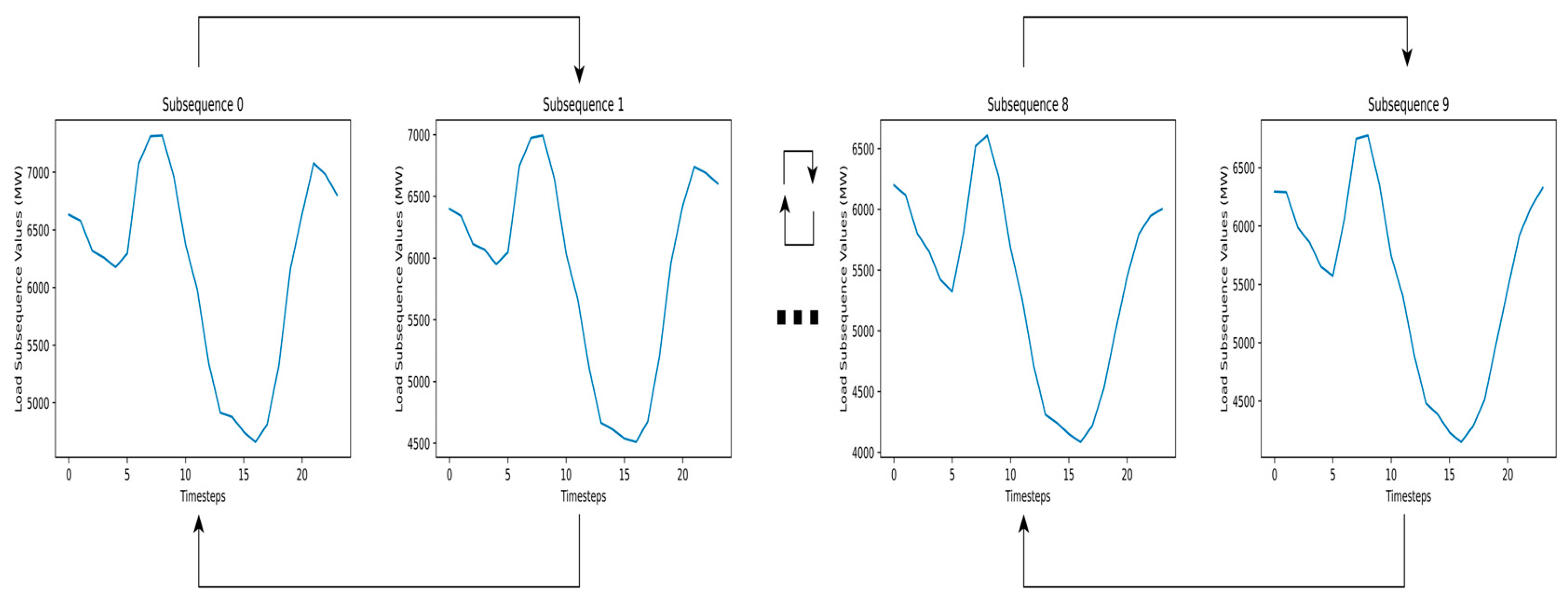
Intuitively, time series chains are temporally ordered sets of time series subsequences. Each subsequence that belongs to a time series chain is similar to the preceding subsequence. However, as the subsequence evolves and the time series chain increases in length, the dissimilarity between the first and last subsequences is likely to increase, resulting in arbitrarily dissimilar start and end points for the chain. The derivation of time series chains depends on the concept of matrix profiles that denote the directionality of evolving subsequence patterns. Matrix profiles focus on the efficient computation and storage of nearest neighbor information through the application of distance metrics. The left and right matrix profiles constitute vectors of z-normalized Euclidean distances between each subsequence and its left and right nearest neighbor respectively. The indices extracted from the left and right matrix profiles are utilized in order to link the subsequences and express directionality. Consequently, the subsequence links could be represented by forward and backward arrows. Forward arrows point to the right nearest neighbor and backward arrows point to the left nearest neighbor. Therefore, within a chain, pairs of consecutive subsequences need to be connected by a forward as well as a backward arrow. Figure 4 presents an example time series chain featuring 24-h load subsequences for the inspection of daily pattern evolution. Time series chain discovery methods utilize the Scalable Time series Ordered-search Matrix Profile (STOMP) algorithm for the efficient computation of left and right nearest neighbor information in scalable time series analysis packages such as STUMPY [62].
Two types of time series chains are supported through this method, the unanchored and anchored chains. Unanchored chains refer to the unconditionally longest chains in a sequence that consist of subsequences containing a specified number of observations. This type of chain does not need a prespecified starting point and aims to express the evolutionary paths that describe general sequence behaviors. On the other side of the spectrum, anchored chains refer to the chains that start with a particular subsequence. This type of chains may not include the longest paths since the specified starting point may be connected to patterns that have a short duration. In the context of load sequence analysis and evaluation, we observe that the study of anchored chains based on specific starting points could either be exhaustive and computationally expensive or incomplete and biased. In both cases, the resulting methods could include patterns describing non-impactful events that are not representative of the evolutionary temporal structure [63]. Consequently, in this study the unanchored chains featuring the minimum average distance between consecutive components are considered for the development of a performance evaluation method in order to examine the quality of pattern conservation and the impact of combinatorial component forecasting on the temporal load structure.

2.4. Problem Framing and Proposed Methodology

This study focuses on the design, implementation and evaluation of combinatorial component-based forecasting methods for day-ahead load predictions influenced by lagged load observations as well as renewable generation sequences. The models developed in this project integrate five different types of estimators including Linear Regression, XGBoost, deep neural network (DNN) following the MLP architecture, LSTM and attention LSTM (Att-LSTM) in order to study the behavior of prominent linear, tree-based and neural network structures. According to the previous outline of research questions and research gaps with regards to the implementation of standalone decomposition methods and the performance evaluation of component-based structures applied on those estimators, there are several observations that contribute towards the conceptualization of this methodology. Firstly, the omission of pitfalls in standalone decomposition-based modeling for the preprocessing phase often overshadows the need to explore the benefits of more robust combinatorial methods, limiting the scope of feature representations. Secondly, the lack of knowledge regarding the shift in the forecasting performance of combinatorial component methods when compared to baseline models often results in the shift of design perspective that leads to the exploration and development of combinatorial estimators. This shift transfers the complexity of the designed methodologies from the early feature preprocessing steps to the design of function approximation structures. Evidently, this approach could prioritize prediction accuracy over interpretability and explainability and use them as a tradeoff in order to achieve lower error metrics. Additionally, this complexity shift could contribute towards the emergence of computational challenges since most methods that experiment on the function approximation structure, introduce new hyperparameters and heuristic methods. Thirdly, the lack of pattern observability during error analysis renders the evaluation of those methods incomplete due to the uncertainty surrounding the quantification of pattern conservation quality. The evolutionary path of the predicted series and its association to the actual sequences often remains unexplored, since the impact of temporal distortions introduced by the learning process is not sufficiently examined.
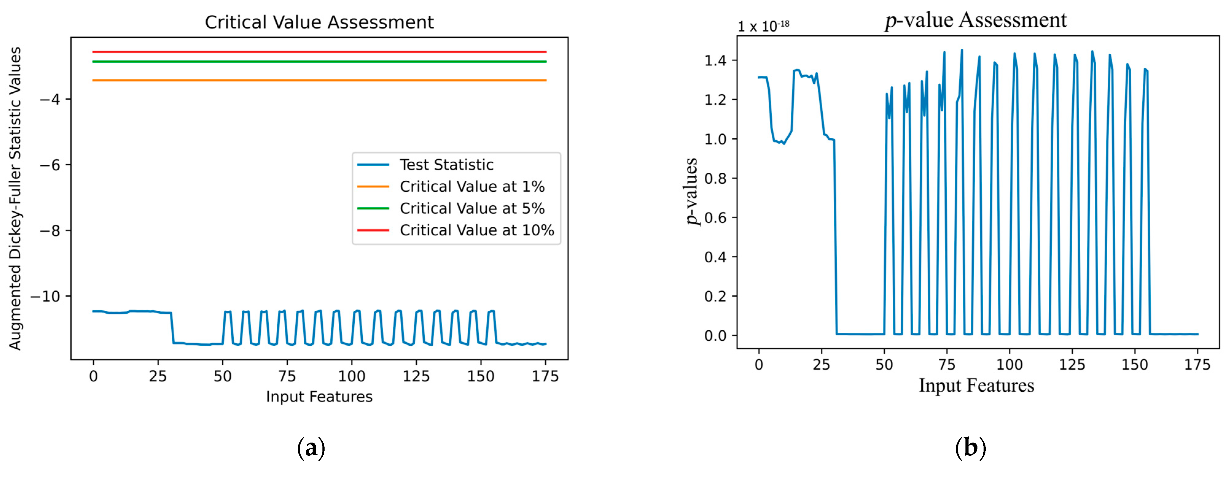
In response to those observations, several modifications to the stages following the dataset preprocessing and error evaluation of decomposition-based forecasting structures are proposed, resulting in the examination of combinatorial component architectures and the development of additional predictive potency metrics. Firstly, after the preliminary dataset preprocessing steps including lag transformation, data cleaning, correlation and stationarity analysis, normalization and train-test splitting for the derivation of the suitable input and output sequence structure in this day-ahead load forecasting task, the unraveling of input features through the STL, SSA and EMD methods produces a dataset including pattern and oscillatory behavior representations in the time and frequency domain. The integration of STL and SSA methods yields a total of six sequence groups featuring diverse representations for the trend, seasonal and residual sequences. On the other side of the spectrum, the integration of EMD considers the first five IMFs representing the most prominent oscillatory behaviors and excluding the ones that fail to capture dominant modes of variability since those random fluctuations could be associated with noise. Consequently, the combination of multiple decomposition methods results in substantial increase of the input feature space dimensions and could introduce additional forecasting uncertainty due to the unknown degree of influence for each individual component sequence. Therefore, following the combinatorial decomposition, a feature selection process is implemented based on the XGBoost estimator. The importance scores extracted from this tree-based method assist in the derivation of an influential component dataset that is close to the dimensions of the original input dataset. Following this step, the component representations are passed to the five forecasting kernels and produce 24 hourly load sequences in the output. Figure 5 outlines the proposed architecture that serves as the core structure for our experiments and highlights the enhancement of the preprocessing stages through the implementation of combinatorial decomposition.
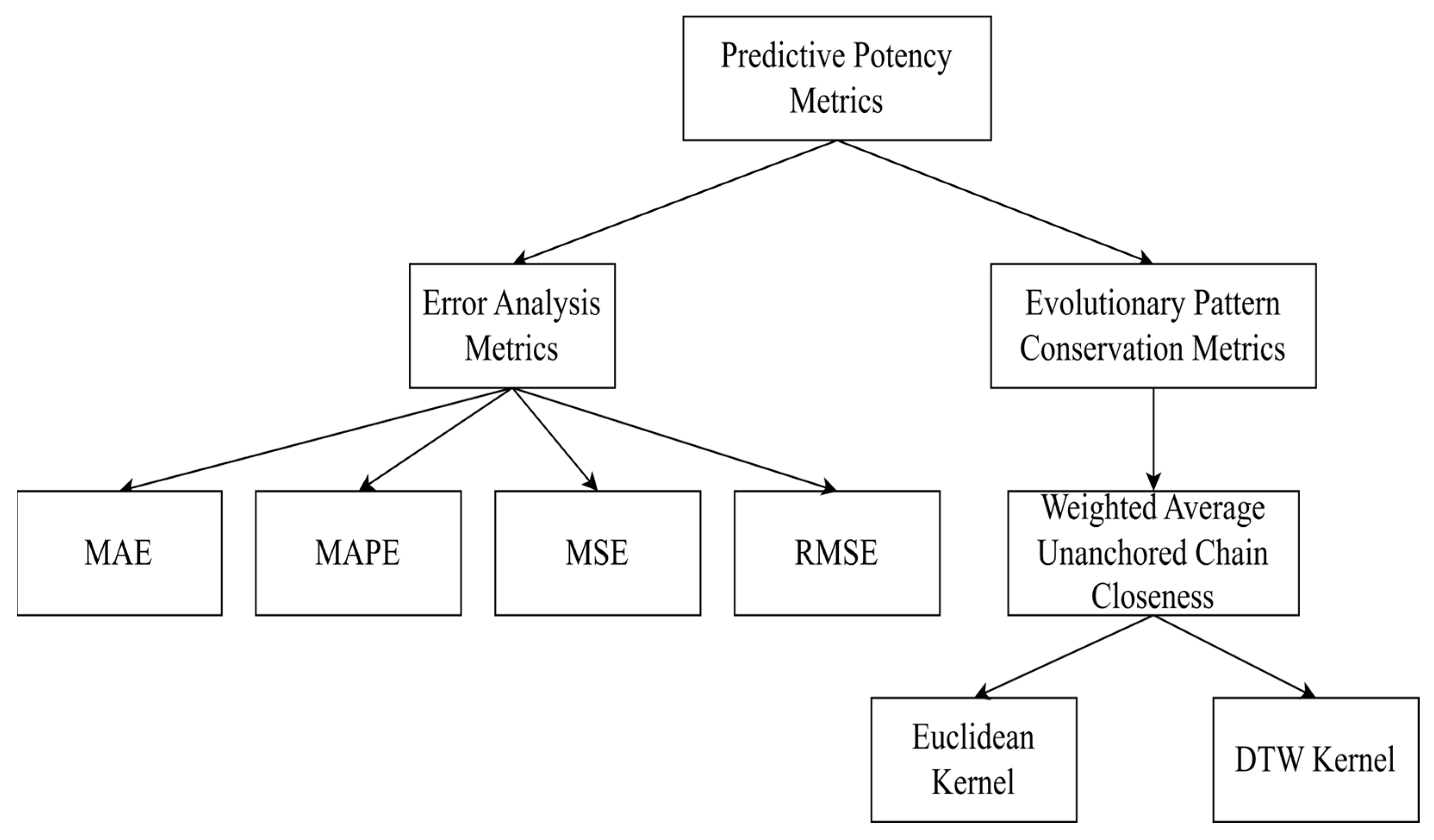
Secondly, the performance evaluation process is enhanced through the introduction of an evolutionary pattern conservation metric that complements the prominent error analysis which includes metrics such as MAE, MAPE, MSE and RMSE. The proposed metric focuses on the unconditionally longest time series chains from each output sequence that share the strongest nearest neighbor relationship in order to examine evolutionary paths formed by actual and predicted subsequences. The closeness between the elements of the chains detected in the actual data are compared to the values of the corresponding indices in the predicted data in order to study the impact of temporal distortions and search for the model that achieves the minimum average distance between those data regions. Since the hourly resolution of observations is utilized in the day-ahead load forecasting task, this study considers the evaluation of pattern conservation quality for unanchored chains formed by daily and weekly subsequences in order to maintain sufficient pattern granularity. The proposed approach utilizes the Euclidean and the Dynamic Time Warping (DTW) distance kernels for the computation of closeness scores for the holistic interpretation of daily and weekly chain deviations. Figure 6 illustrates the extension of the evaluation stage and highlights the inclusion of the pattern conservation quality metric. In the following subsections, the detailed configurations of the proposed forecasting models as well as the definitions of the evaluation metrics will contribute towards the thorough understanding of the experiments carried out in our case study.

2.5. Performance Metrics

2.5.1. Error Analysis

In this subsection we present the definitions of prominent error metrics in decomposition-based load forecasting tasks as well as an overview of their role towards the interpretation of forecasting performance in order to highlight their usage within the scope of this research work. First, Mean Absolute Error [64] evaluates the accuracy of those forecasting models through the calculation of average absolute differences between each predicted and actual value of each output sequence. This metric constitutes an interpretable loss function that provides a natural and scale-dependent measure of error. MAE is commonly utilized in load forecasting tasks for model comparison due to its simplicity and robustness with regards to outliers. However, the model evaluation process through MAE as a standalone metric may not be considered complete since the derived scores do not consider the magnitude and direction of errors as impact factors for this performance examination. Given the predicted values y i and actual values x i in a sequence of n observations, the mean absolute error is computed by the formula:
M A E = i = 1 n y i x i n
Second, Mean Absolute Percentage Error [65] is a prominent metric in regression model evolution that expresses the error as a percentage through the calculation of absolute percentage differences between the actual and predicted values, divided by the total number of observations. This metric is scale independent and produces a measure of relative error for the studied models, rendering it highly interpretable and thus suitable for baseline and combinatorial component model comparisons in this research work. Challenges associated with MAPE include the sensitivity of the function to small actual values that could lead to large percentage errors, the limitations with regards to zero division that results in undefined values and denotes difficulty in handling values that are close to zero and the potential introduction of bias in the scenario where large percentage errors are overweighted due to the existence of outliers or extreme values. Given the information for the calculation of MAE, MAPE scores are calculated through the following formula:
M A P E = 100 n i = 1 n y i x i x i
Finally, the quadratic loss functions of Mean Squared Error [66] and Root Mean Squared error [67] are included in order to examine the impact of large errors. The values of MSE are derived from the squared differences between actual and predicted values, divided by the total number of observations. Extending this definition, RMSE values are obtained through the square root of the calculated MSE scores. Both metrics are expressed in the same units as the target sequences, rendering them equivalently interpretable and suitable for the performance comparison presented in this case study. It is worth noting that both metrics are sensitive to outliers and extreme values and tend to penalize large errors through those square differences. Additionally, the co-inspection of MAE and RMSE could provide useful insights with regards to the occurrence of large errors and the degree of error variation, indicated by the proportional difference between the metric values. Given the information for the calculation of the previously defined metrics, MSE and RMSE values are computed by the following formulae:
M S E = i = 1 n y i x i 2 n
R M S E = i = 1 n y i x i 2 n

2.5.2. Evolutionary Pattern Conservation Quality

It is evident that while the combined examination of MAE, MAPE, MSE and RMSE could provide a robust interpretation of predicted value deviations from the actual sequence, the consistency in the representation of important patterns and the impact of distortions in the evolution of time series are not explicitly explained. Furthermore, it is observed that this error analysis is typically enhanced by sequence visualizations that focus on the point-to-point comparison of important data regions, selected non-deterministically for the purposes of each learning task while mainly reflecting domain knowledge. As a result, the knowledge extracted from those visualizations may not enrich the interpretation of model performance beyond the characteristics associated with the mathematical properties of those metrics. These observations highlight the need for intuitive and interpretable metrics that focus on the quality of the captured patterns as they evolve over time. In forecasting models involving the integration of decomposition-based methods, the need for pattern-oriented metrics becomes accrescent since the boost in accuracy is mainly attributed to component representations that assist the forecasting structures in the process of learning evolutionary paths and hidden feature relationships. Consequently, researchers in this sector need to be able to identify models that exhibit divergent evolutionary behaviors and evaluate drifting motifs. Therefore, in this section we introduce a flexible and interpretable metric based on the data mining primitive of time series chains for the quantification of pattern conservation quality considering important sets of subsequences.
The metric introduced in this study, considers the weighted average distance between the most compact unanchored time series chains identified across the actual target output sequences and the corresponding predicted values derived from the load forecasting structures. The characteristics of this metric assists in the interpretability of time series pattern evolution and the impact evaluation of temporal distortions, denoting the ability of the predicted sequences to preserve the evolutionary paths of the original target series accurately and consistently through time. This metric is labeled as the Weighted Average Unanchored Chain Divergence (WAUCD) and utilizes two different distance kernels to derive the scores for the studied chains. Following the detection of the unanchored time series chains with the strongest nearest neighbor relationships between subsequences of user-defined interval length through the utilization of the efficient STOMP implementation in the STUMPY package, the distance between each actual subsequence c k and the corresponding predicted subsequence c ^ k could be calculated through a configurable distance kernel function through the formula:
d k = d i s t ( c k , c ^ k )
For the purposes of this study, the Euclidean and the dynamic time warping functions are considered as prominent distance kernels for the derivation of subsequence distances. The integration of the Euclidean distance metric yields a more pessimistic point-to-point similarity score and imposes strict assumptions with regards to the equality of subsequence length. On the other side of the spectrum, dynamic time warping yields more flexible and optimistic scores due to the minimization of alignment-based distortions and enables further meta-processing that is no longer restricted by the subsequence length. The average element-wise distance score s i for the unanchored chain detected in sequence i of m total subsequences is defined as:
s i = k = 1 m d k m
In the univariate output scenario, this average distance score could be considered for simple model comparison. However, more impactful insights with regards to time series evolution could be extracted from the multivariate extension of this metric. Considering the average distance scores for the unanchored chains detected in sequences representing different timesteps of the target output, a weighting strategy could be formed in order to denote the importance of pattern conservation quality throughout the target temporal structure. This strategy could penalize the distortions and chain divergence exhibited in distant timesteps, emphasizing model stability and consistency. Therefore, weights w i could be defined proportionally to the temporal position i of each of the z output sequences through the following formula:
w i = i z
Subsequently, the scores for WAUCD are computed by the weighted average formula that gradually penalizes the scores of distant time steps by emphasizing the importance of maintaining significant chain closeness as the temporal gap between the last observed input sequence and the target output sequence widens:
W A U C D = i = 1 z s i w i i = 1 z w i
The interpretation of this metric indicates that a multiple-output model forecasting z time series yielding low WAUCD for p-length subsequences exhibits an evolutionary behavior that matches the patterns observed in the actual data accurately. High WAUCD scores express instabilities attributed to the larger errors of distant time steps. The proposed metric is highly configurable for different types of learning tasks since there is a high degree of freedom in the selection of structural parameters and evaluation kernel functions. For the purposes of a given learning process, the subsequence length as well as the chain length and the neighboring subsequence strength could be adjusted in order to examine different task-specific temporal patterns. Additionally, alternative weighting strategies and different kernel functions could be considered for the derivation of different result interpretations.

2.6. Case Study and Experiments

2.6.1. Dataset Overview and Preprocessing

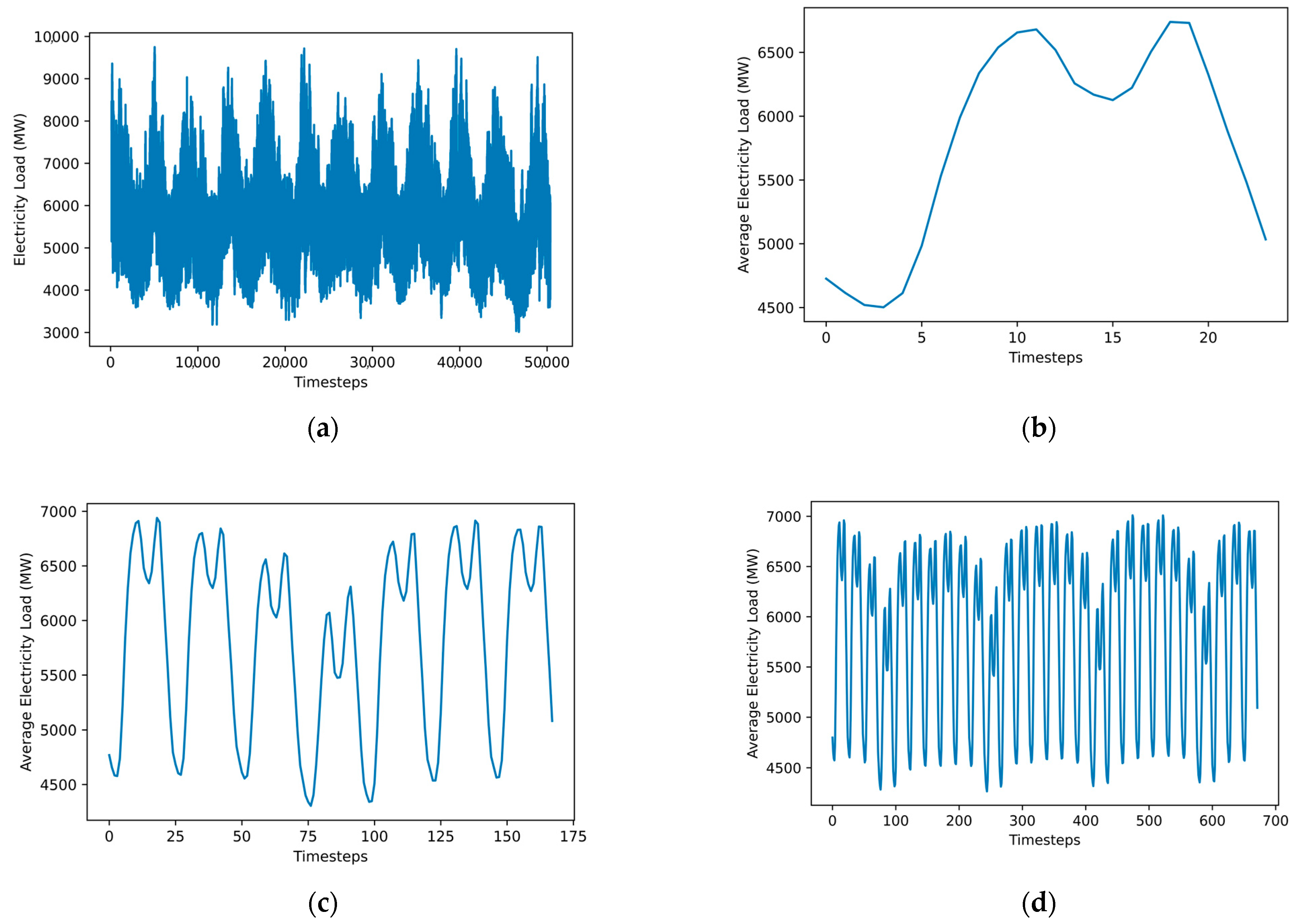
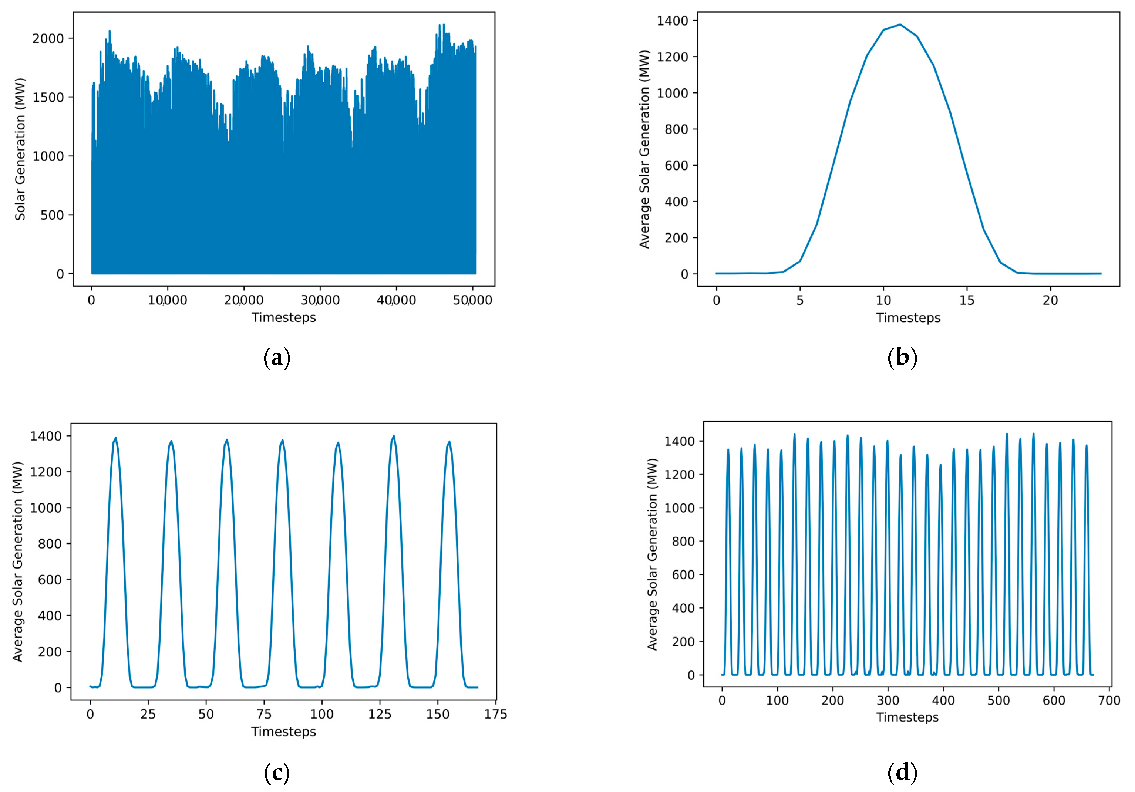
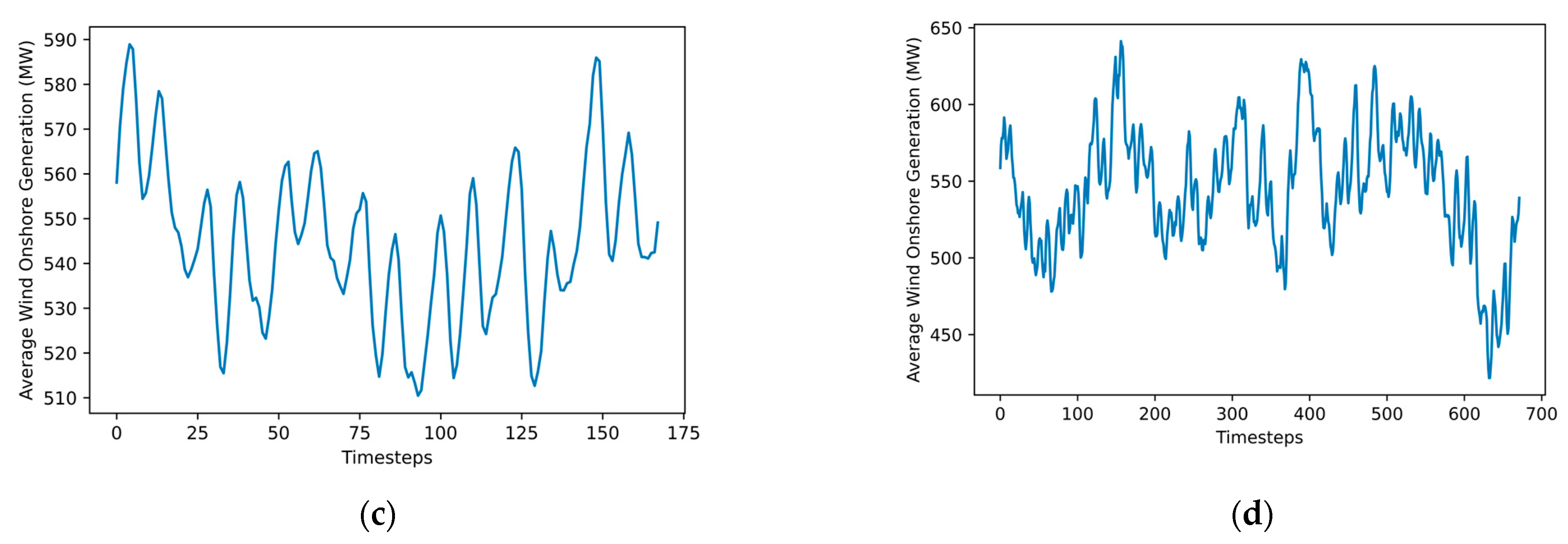
In this subsection, we present the core information with regards to the dataset and outline the preprocessing stages utilized in the implementation and evaluation of our proposed forecasting approach. The publicly available dataset utilized in our experiments was obtained from the Open Power System Data platform [68]. This dataset contained time series sequences for the Greek power system covering the period between 31 December 2014 23:00 and 30 September 2020 23:00 and consisting of a total 50,400 observations in hourly resolution. These sequences represent the total actual load as published on ENTSO-E Transparency Platform by transmission system operators and power exchanges, the actual solar generation and the actual on-shore wind generation in Greece, measured in MW. Figure 7, Figure 8 and Figure 9 present the line plots and the respective average daily, weekly and monthly profiles for each feature considered in this study in order to provide a concise overview of the dataset in several resolutions of hourly timesteps that are relevant to short-term load forecasting tasks. This feature inspection highlights the strong and consistent oscillatory behavior of the total load and solar generation. Additionally, it illustrates the pronounced increasing trend of wind generation which could be attributed to a combination of strategic investments, supportive policies and international backing that contributed towards the significant growth of wind capacity during this time period.
Since the studied learning task considered the prediction of day-ahead load based on historical load and renewable generation sequences, the initial dataset was restructured in order to include 100 features for each initial sequence, formed through the sliding window method for the derivation of 99 additional lags [69]. Therefore, the target output consisted of the 24 most recent load sequences and the input consisted of the remaining 76 load lags as well as 200 sequences for solar and wind generation. Missing values were removed from the dataset, resulting in 50,224 hourly observations. Furthermore, the dataset was split into the training set and the test set following the 80–20% split that is commonly used in the hold-out validation approach [70]. The resulting sets were normalized through the min-max normalization method [71] in order to scale values between zero and one and prevent scale-dependent bias during the learning process. Moreover, it is worth noting that since we focused on the evaluation of estimator performance through the integration of a combinatorial decomposition method, we aimed to verify that the participating input features express general linear associations to the target sufficiently well as a baseline, thus minimizing the impact of uncorrelated sequences and discrepancies in the linear structure. This initial filtering could assist in the interpretation of the performance boost stemming from the discovery of additional nonlinear relationships and evolving patterns within the component representations. Consequently, a threshold method utilizing the Pearson correlation analysis [72] coupled with a linear regressor was implemented for the examination of training performance based on the selected features. Table 1 presents the training error evaluation for 0.6, 0.8 and 0.9 as the minimum absolute correlation thresholds. The threshold value of 0.6 corresponds to the exclusion of wind generation sequences. The threshold of 0.8 corresponds to the subsequent exclusion of solar generation sequences and the value of 0.9 corresponds to the 24 lagged load sequences with the highest absolute correlation. This analysis denoted that the exclusion of wind generation sequences resulted in the derivation of a more compact and clearly associated training set with an acceptable minimum correlation threshold value of 0.6, without resulting in substantial performance deterioration due to dimensionality reduction.
Following this step, a statistical stationarity analysis was performed through the Augmented Dickey Fuller (ADF) test [73] in order to verify that the resulting 176 input sequences were stationary. Stationarity could affect the performance of decomposition methods, since stable statistical properties for the studied sequences could prevent model assumption violations during component extraction and reduce value variability with regards to spurious fluctuations that could render the detection of trend and seasonality more challenging. Additionally, stationarity could contribute towards the clear isolation of the residual component without the erroneous inclusion of systematic patterns that could result in correlated and heteroscedastic errors as well as biased parameter estimation. Consequently, through the inspection of the critical value assessment and the p-value assessment we verified that the input sequences were stationary. Figure 10 indicates that the test statistic value is significantly lower than the critical values for all sequences and the p-value is lower than 0.05, rendering the input dataset stationary.

2.6.2. Decomposition and Estimator Configuration

The proposed methodology applied STL, SSA and EMD on the preprocessed dataset. Following the previously presented model structure, STL and SSA derived three components for the representation of trend, seasonal and residual sequences while EMD considered the first five IMFs in order to represent the most prominent oscillatory patterns in the data. This decomposition step resulted in the increase of dataset dimensions, producing 1936 component input sequences. A feature selection method based on importance scores extracted from the XGBoost algorithm was applied in order to reduce the dimensions of the input dataset and retrieve the most influential component representations. Therefore, based on the optimal split of the tree-based learners in this ensemble method, the top 200 sequences were selected for the day-ahead load forecasting task in order to define a combinatorial component dataset that was similar to the preprocessed input in terms of dimensions.
This case study considered five estimator kernels utilizing common parameter configurations in order to analyze the performance of different machine learning architectures on the original and the combinatorial component dataset. A linear regressor following its default configuration was trained in order to obtain a naïve estimate from the linearly approximated sequences and an XGBoost method with default parameter values extracted the baseline tree-based ensemble performance. In terms of neural network structures, a deep neural network and two LSTM network variants were considered. The deep neural network followed the MLP structure and featured the input layer, two hidden layers and the output layer. The first hidden layer followed the dimensions of the input and included 176 neurons for the base case and 200 neurons for the combinatorial component scenario while utilizing the Rectified Linear Unit (ReLU) activation function. The second hidden layer halved the number of neurons to 88 and 100 respectively and utilized a linear activation function. The output layer included 24 neurons, each one producing an hourly sequence for the day-ahead load forecast through linear activation. The first LSTM network variant represented a simple LSTM network that included the input layer, an LSTM layer and a dense output layer. The LSTM layer followed the dimensions of the input including 176 LSTM cells for the base case and 200 cells for the combinatorial component scenario while utilizing the hyperbolic tangent activation function [74]. The dense output layer included 24 processing units for the prediction of each hourly sequence through linear activation. The second LSTM network variant extended the simple LSTM structure through the integration of an attention layer that derived context vectors from the weights of the returned hidden states that were extracted from the previous LSTM layer, following the concept of Bahdanau attention [75]. Consequently, the dimensions of the attention layer matched the dimensions of the LSTM layer. This variant investigated the isolated predictive potency of context vectors derived from the original as well as the component-based input. Figure 11, Figure 12 and Figure 13 illustrate the structure and the forward information flow of the previously described neural network structures.

2.6.3. Experiments and Evaluation Strategy

This study examined and compared the performance of LR, XGBoost, DNN, LSTM and attention LSTM estimators on the original preprocessed dataset and on the dataset featuring important components derived from the combinatorial decomposition method. The training of XGBoost and LR was completed based on default convergence criteria and for the neural network models the number of total epochs was set to 4000 in order to provide ample space for the effective convergence of the learning processes. Furthermore, for the prevention of overfitting, early stopping [76] was implemented featuring a patience interval of 100 epochs. This interval provided the necessary space for validation loss reduction and constituted the proportionally small segment of the learning task where the models attempted to achieve consecutive performance improvement. The DNN model utilized a stochastic gradient descent optimizer with learning rate of 0.0005, decay rate of 0.000001 and momentum of 0.8. The LSTM models utilized the Adam optimizer [77]. Additionally, the batch size parameter for the neural network models was set to 72 training samples. The selection of prominent training approaches, static commonly used parameter values and structural configurations contributed to the consistency of the results, assisting in the deterministic comparison of the estimator performance before and after the derivation of influential input components.
The evaluation strategy for the studied models included the monitoring of loss functions for the training and test set, the examination of error metrics and the interpretation of pattern conservation quality for the forecasted sequences. The error analysis considered the prominent metrics of MAE, MAPE, MSE and RMSE for the robust interpretation of data point divergence. The analysis of pattern conservation quality utilized the proposed WAUCD metric for the longest chains including 24-h and 168-h strongly related subsequence elements. This approach examined the aftermath of the forecasting process with regards to the preservation of daily and weekly patterns. Moreover, the Euclidean and DTW distance kernels were considered for the calculation of the WAUCD scores in order to provide a more flexible interpretation of the resulting distances. The experiments presented in this study were implemented in Python 3.8.18, using the packages pandas 2.0.3 and numpy 1.24.3 for data processing. Additionally, statsmodels 0.14.0, emd 0.6.2 and pyts 0.13.0 were selected for the implementation of the decomposition methods. The packages scikit-learn 1.3.0, tensorflow 2.10, keras 2.10 and xgboost 1.7.3 were utilized for the implementation of the forecasting models. In the evaluation stages, stumpy 1.12.0, and tslearn 0.6.2 were utilized for the inspection of time series chains. Lastly, matplotlib 3.7.2 was selected for result visualization. It is worth noting that any model parameters not mentioned in this section follow the default values of those packages. The baseline as well as the combinatorial component models and the corresponding experiments were executed on a desktop computer with an AMD Ryzen 1700X processor, 8 gigabytes of RAM, and a NVIDIA 1080Ti graphics processor. The code of this study, containing the preparation of the dataset as well as the analysis of the proposed day-ahead load forecasting approach and evaluation method, is publicly available on GitHub [78].

3. Results

This section presents a detailed performance overview for the studied forecasting approaches, examines the behavior of the baseline estimators that utilized the compact dataset of load and solar generation input sequences and compares this baseline performance with the performance of the estimator structures that selected influential input components from the combinatorial decomposition approach. Following the evaluation strategy outlined in the previous subsection, the results are split into three segments, covering three different evaluation perspectives. The first segment addresses the training and test set behavior through the examination of loss functions towards the convergence of the models. This segment includes the learning curves of iterative optimization methods, focusing primarily on the training paths of the tree-based XGBoost algorithm as well as the neural network structures since there are valuable insights that could be extracted for the thorough interpretation of these complex learning processes. The second segment addresses the error analysis of the produced sequences on the test set, highlighting the performance of the models on each sequence and providing the average multi-output error metrics. Lastly, the third segment examines the quality of pattern conservation and its shift after the implementation of the proposed forecasting structure through the time series chain-based metric.

3.1. Learning Curve Examination

The side-by-side comparison of train and test loss over the total number of training iterations could provide useful information towards the evaluation of learning stability, overfitting or underfitting tendencies and the degree of smoothness as the models approach convergence. Figure 14, Figure 15, Figure 16 and Figure 17 present the learning curve comparison between the baseline models utilizing the preprocessed load and renewable generation sequences and the models utilizing the most important component-based inputs. It is evident that all models were sufficiently complex, achieving balance between bias and variance, since there were no significant gaps observed between the training and test loss functions. This observation indicates that the studied models did not exhibit overfitting or underfitting and managed to extract patterns from the given sequences, learning from their temporal structures. Consequently, the consistency and robustness of these learning curves could contribute towards the clear interpretation of behavioral changes that occur due to the utilization of the combinatorial decomposition method coupled with the importance-based feature selection strategy. Influential components benefit the learning process of each estimator differently, rendering this comparison important for the evaluation of this forecasting performance shift. The baseline XGBoost regressor exhibited a trend of increasing divergence between the training and test loss curves, denoting that additional boosting rounds could widen the gap between them, resulting in overfitting. The important component-based XGBoost estimator suppressed this behavior, resulting in a narrower gap and lower loss function values for the same number of boosting rounds without compromising the smoothness of training. The DNN architectures exhibited similar behaviors for both types of inputs in terms of learning stability since the training irregularities in the first 25 epochs and the small fluctuations in the test curve appear in both scenarios. Combinatorial component-based input mainly affected the generalization capability of the DNN since the estimator achieved additional improvements of the test loss, triggering the early stopping mechanism after an extended number of epochs. Lastly, the behavioral shift of both LSTM variants highlighted the improved learning smoothness during initial epochs and the enhanced generalization capability stemming from the utilization of the proposed approach. Therefore, this preliminary examination of iterative optimization methods outlines the overall positive impact of the proposed strategy in the day-ahead load forecasting task, denoting important refinements in the predictive potency of tree-based and neural network structures.

3.2. Error Analysis

In this subsection, a detailed overview of error scores is presented, including the MAE, MAPE, MSE and RMSE metrics for each output sequence as well as the average scores for the studied estimators. The inspection of error metrics for each sequence in the 24-h interval could provide useful insights towards predictive stability and the impact of large errors through time. The average multi-output scores illustrate the overall model performance, providing a concise and descriptive evaluation strategy for the studied forecasting horizon. Figure 18, Figure 19, Figure 20, Figure 21 and Figure 22 present the side-by-side comparison of error metrics for each hourly sequence between the baseline and proposed models. The proposed models utilizing the combinatorial decomposition method are prefixed with “CC” in the following graphs.
The examination of the hourly error metrics leads to several observations regarding the performance of the studied models. The increased focus towards the representation of non-linearities through the combinatorial decomposition approach had a negative impact on the performance of the linear regressor, resulting in inconsistent hourly error metrics and the rapid escalation of error scores in distant timesteps. This error analysis renders the linear regressor as the least compatible kernel estimator for the component-based dataset due to the overall unpredictability of the error profile which suggests that some information could be interpreted as random noise during the learning process. The tree-based XGBoost model and the neural network architectures benefited significantly from the rich and clear representation of patterns in the component-based sequences and yielded substantially improved error scores while maintaining a stable error profile, exhibiting the expected increasing error trend for distant timesteps within the 24-h interval. The DNN structure and LSTM variants yielded the most substantial error improvements, with the DNN achieving impressive performance for the first six hourly sequences and the LSTM variants producing more accurate forecasts for the last six hourly sequences. The co-inspection of MAE and RMSE scores for the stable forecasting models verifies the lack of large errors and indicates a small degree of error variation in both input strategies since the values of those metrics do not diverge drastically.
Following the hourly performance overview, the average multiple output performance of the models is outlined in Table 2. The average error scores indicate that the combinatorial decomposition approach led to the substantial improvement of the models that are able to process the non-linearities of the dataset. The DNN structure performed well in both scenarios and the LSTM variants achieved the most substantial error reduction due to the efficient prediction of distant timesteps. The single-layer combinatorial component LSTM yielded the best performance across all studied estimators and the attention LSTM variant demonstrated that robust predictions could be derived from the simplified context vector structure without significant accuracy loss. Additionally, the co-inspection of the average RMSE and MAE for the XGBoost and neural network structures illustrates the overall reduction in error variation. Furthermore, the large difference between the average RMSE and MAE scores of the linear regressor denote the instability and unreliability of this kernel estimator.

3.3. Pattern Conservation Quality

In this subsection, the evolutionary patterns of the load sequences are studied through the data mining primitive of time series chains for the quantification and evaluation of conservation quality on the longest strongly related subsequences within the given temporal structures. This analysis focused on daily and weekly subsequences that belong to those unanchored chains for each actual and predicted hourly sequence. Moreover, the Euclidean and DTW are selected as distance kernels for the holistic derivation of distance scores. In the first stage of this analysis, the side-by-side comparison of the average chain similarity for daily and weekly unanchored chains detected in each hourly sequence is presented in order to identify differences on the impact of temporal distortions for the baseline and combinatorial component models. The respective Euclidean and DTW scores are plotted in Figure 23, Figure 24, Figure 25 and Figure 26.
This evaluation stage highlights the improvement in the stability and the consistency of evolutionary time series behaviors in the predicted sequences that stems from the integration of the proposed combinatorial decomposition method. The fluctuations of the distance scores coupled with the increasing trend through time indicate that the forecasted subsequences exhibit significantly divergent behaviors when compared to the actual subsequences the at the corresponding timesteps. This phenomenon could compromise the interpretation of time series evolution, resulting in interpretability and explainability deterioration at later time steps. The integration of the combinatorial component sequences contributed to the flattening of distance curves and the suppression of the increasing trend as the distance values are reduced across the stable neural network kernel estimators. The LSTM variants exhibited the most stable performance across all hourly sequences. Furthermore, it is worth noting that the XGBoost model exhibited distinctly higher distance metrics in both baseline and combinatorial component scenarios. The clear outlier in this approach is the linear regressor. This estimator was not capable of processing the sequences representing non-linearities efficiently, resulting in more erratic fluctuations and high distance scores.
The second stage of this evaluation process considers the proposed WAUCD metric which encapsulates the average multiple output pattern conservation quality for the studied models and penalizes the distortions occurring on distant timesteps. Table 3 and Table 4 present the WAUCD scores with regards to the DTW metric and the Euclidean distance, respectively. The scoring tables consider daily and weekly patterns.
The examination of the WAUCD scores consolidates the overall improvement of the kernel estimators in producing evolutionary paths that are significantly closer to the paths of the actual sequences when the influential component inputs are integrated. Additionally, this score reduction reflects the enhanced resilience of the proposed models towards temporal distortions since the emphasis on the chain closeness in distant timesteps imposes a restrictive perspective of pattern similarity. Since model performance is expected to deteriorate in the prediction of timesteps farther in the future due to the challenges of concept and data drift, the attention to those divergent subsequences provides a robust closeness estimate that covers the most sensitive target regions of the multiple-output estimators. Similar to the first stage, the LSTM variants and the DNN model yield the most substantial average distance reduction, rendering them the most compatible kernels for the combinatorial decomposition approach. Lastly, the inability of the linear regressor to learn from the multiple-component input structure resulted in WAUCD scores that greatly surpassed the baseline. Moreover, the impact of the combinatorial decomposition approach on the pattern preservation quality could be observed through the visualization of the unanchored chain start and end subsequences. The following sample visualizations presented in Figure 27, Figure 28, Figure 29 and Figure 30 explore the divergence of the start and end subsequences extracted from the daily and weekly unanchored time series chain of the last time series in the studied interval. Since this sequence refers to the last timestep of the 24-h period, forecasting distortions are expected to be easily discernible due to the larger magnitude of errors. Therefore, the effect of the combinatorial decomposition method could be observable at an equivalent level of clarity from those graphs.
The inspection of those visualizations indicates that the integration of important component-based features resulted in the consistent modeling of time series patterns since the neural network models and the tree-based estimator produce forecasted series that exhibit fewer fluctuations. Consequently, the interpretability of the estimated patterns is reinforced due to the enhanced error stability. Evidently, the forecasted series did not represent a drastically different evolutionary behavior when compared to the actual output values. The weekly subsequence elements highlight the negative impact of the proposed methodology on the performance of the linear estimator, where the inaccurate interpretation of specific data regions resulted in greatly increased output errors.

4. Discussion

This research project introduced an importance-driven combinatorial decomposition approach for day-ahead load forecasting and evaluated the performance of several kernel estimators in terms of prediction error and pattern conservation quality through a case study. This case study examined the relationships between hourly target sequences representing the total Greek electricity load and input time series representing total renewable generation and lagged load observations. The error analysis focused on the prominent error metrics of MAPE, MSE, RMSE and MAE in order to extract error profiles for each hourly target sequence and study the average model performance in the baseline and combinatorial component scenarios. The evaluation of pattern conservation quality integrated time series chain concepts in order to introduce an intuitive and flexible metric for the monitoring of evolutionary path divergence between the actual and predicted series. The hourly distance-based analysis of average chain similarity provided a fine-grained overview of the distortion profile for each estimator and the proposed WAUCD metric enabled the concise description of overall model divergence through the inspection of the most important daily and weekly unanchored chains.
The experiments denoted that the utilization of influential components, improved model generalization and reduced the error of load predictions substantially for estimators that are capable of extracting complex non-linear time series patterns. The inspection of learning curves highlighted the extended improvement of loss function values and the overall smoothness of training. The examination of error profiles illustrated the improved model stability and verified the significant reduction of error metrics for each hourly sequence. The overview of average error metrics denoted that the combinatorial component LSTM (CC-LSTM), attention LSTM (CC-Att-LSTM) and DNN (CC-DNN) models are the most compatible estimators for the implementation of the proposed forecasting approach since they yielded the most significant error metric improvement. The CC-LSTM yielded the improved MAPE value of 1.830 surpassing the baseline LSTM MAPE of 3.444. The CC-Att-LSTM and CC-DNN achieved MAPE values of 1.889 and 1.949 which were substantially lower than the respective baseline values of 3.596 and 3.404. The shift in error metrics highlights a significant boost in predictive potency that surpasses baseline improvements observed in relevant research efforts [34,35,38,39,40,41,48]. Through this error analysis, we observed that while the DNN estimator was able to perform well for the prediction of the first several sequences in the baseline and the component-based scenarios, the LSTM structures benefited from the unraveling of features and were able to produce significantly more accurate sequences near the end of the studied interval, leveraging their intrinsic characteristics with regards to long time dependencies. The inspection of evolutionary patterns through the evaluation of unanchored time series chains showed the enhanced resilience of component-based estimators with regards to temporal distortions. The average chain similarity scores for each load sequence indicated the increased stability and consistency of pattern conservation through the integration of the proposed approach. Moreover, the overview of WAUCD scores elucidated the overall ability of studied estimators to capture the actual evolving behavior of load. The coupling of the proposed decomposition strategy with LSTM variants resulted in efficient pattern matching, since CC-LSTM and CC-Att-LSTM yielded 519.105 and 548.654 for daily subsequences as well as 1316.265 and 1347.603 for the respective weekly subsequences with regards to the DTW distance metric. Similarly, the Euclidean scores highlighted the robustness of those two architectures with 590.069 and 634.231 for daily subsequences as well as 1636.850 and 1701.846 for weekly subsequences. Lastly, it is worth noting that the component-based inputs introduced more complex sequences in this forecasting task. As a result, the interpretability of neural network structures remains challenging due to their black-box nature that stems from their intrinsic characteristics such as their non-linear transformations, complex layered structure and high parameter dimensionality. Furthermore, simpler approaches such as the linear regression exhibited performance deterioration.
This study explored the impact of component fusion highlighting several advantages and disadvantages of this method based on the behaviors of different types of estimators. The proposed method merged the assumptions of several decomposition methods and produced inputs that reflected the most influential representations of patterns and oscillatory electricity load and renewable generation behaviors. The combined properties of those methods contributed towards the fine-grained interpretation of complex time series behaviors and resulted in significantly more accurate forecasts that maintain the evolutionary temporal structure of the actual target sequences. This was a crucial step towards the thorough interpretation of system dynamics through time since this approach streamlined the error profiles and suppressed the potential emergence of misleading or divergent patterns due to overestimations or underestimations. Consequently, the forecasted time series would be more useful towards meta-processing techniques due to the improved quality of the preserved temporal structure. It is worth mentioning that the forecasting series processing through time series chain concepts enabled the emergence of context-based analysis, complementing and expanding on the observations extracted from the error analysis. This processing step is erroneously omitted in most decomposition-based studies, resulting in the limited implicit deduction of pattern conservation quality. Moreover, the flexibility in the configuration of this approach could contribute towards the development of robust estimators that are compatible to the learning task in terms of structural and training parameters.
On the other side of the spectrum, the datasets processed through this method become increasingly complex since the component-based inputs represent intricate time series behaviors. This component fusion could be incompatible with some estimator structures due to their intrinsic approximation capabilities. Therefore, the lack of simplicity during the early processing steps encourages the integration of complex and more resource intensive estimators, increasing the computational requirements for the day-ahead load forecasting task. Furthermore, it is worth noting that the implementation of a combinatorial component extraction method in the input may not increase the total execution time prohibitively since the previously discussed decomposition methods typically yield fast and moderate execution times on datasets containing adequately explainable historical features, ranging from several seconds to several minutes. Additionally, the integration of XGBoost in the derivation of importance scores aims to streamline the component selection process under an estimation framework that is well-known for its convergence speed. The proposed method could be easily parallelizable since the main interaction between time series components occurs at the XGBoost regressor. Therefore, the computational requirements could be minimized to consider solely the slowest decomposition method, the XGBoost importance extractor and the kernel estimator. In this case study, the slowest decomposition method would be the EMD due to the intensive computation of intrinsic mode functions and the slowest selected kernel would be the Attention LSTM due to its more complex architecture when compared to the other estimation kernels. However, limiting the number of the extracted mode functions to the ones that describe the most prominent oscillatory behaviors for our experiments resulted in acceptable execution times of the sifting algorithm that were consistently and significantly lower than the input sampling rate, allowing for model recalibration as new observations could be added to the historical dataset for all studied regressors.
Future research work could expand on the fusion of decomposition methods and explore several variants of the studied methodologies in order to improve the performance of different forecasting tasks. Additionally, since the extraction of context vectors resulted in promising error and pattern conservation scores, meta-processing attention-based architectures could learn from the residual pattern divergence and derive simplified complementary feature sets that could refine the performance of the baseline models further. Lastly, there are several possible extensions to the proposed evolutionary pattern examination process that could contribute to the integration of more time series chain concepts. Depending on the studied horizon and the temporal characteristics of the target variables, the detection region and chain length could be adjusted in order to outline the long-term impact of specific data anomalies. Alternatively, the contextual analysis of chain evolution could assist in tracing the pattern changes that contributed to error profile changes in distant timesteps and evaluate the strength of causal relationships between important subsequences for the forecasted output.

5. Conclusions

The day-ahead load forecasting task involves the analysis of complex time series patterns and the processing of non-linear relationships between the input and the output. The decomposition of time series features contributes towards the efficient identification of patterns and the development of compatible load estimator architectures through the isolation of noise and the thorough understanding of trends. However, the challenges of standalone decomposition methods limit the generalization capabilities and the adaptability of those estimators, often resulting in assumption-sensitive and biased models that provide an incomplete or distorted interpretation of the underlying temporal structures and system dynamics. Therefore, the research shift towards combinatorial decomposition approaches and the behavioral study of different estimator types could lead to the development of more stable and accurate forecasts through the holistic overview of important feature representations. Additionally, it is important to note that while error analysis constitutes a robust and prominent strategy for the quantification of estimator accuracy in this learning task, it could be considered a limited and incomplete approach for the quantification of decomposition impact since the consistency in the interpretation of patterns and the evolution of the predicted sequences are often implicit and ambiguous. Consequently, evaluation methods that address the evolution of patterns and the similarity of important subsequences could complement the error metrics and extract meaningful insights that enrich the interpretability of decomposition-based structures.
In this work, a robust combinatorial decomposition approach was developed to explore the performance benefits of well-known estimators through the importance-based fusion of STL, SSA and EMD methodologies for the extraction of influential input feature representations and a novel evaluation metric was introduced for the robust and configurable assessment of output evolution. The main conclusions of this work were the following:
  • The important spectrum of nonlinear components enhanced the generalization capabilities of tree-based and neural network architectures since the diverse fine-grained representation of the input resulted in lower and more stable error profiles.
  • The LSTM and DNN architectures benefited the most from this combinatorial method since they were able to capture the exposed nonlinearities more efficiently. The CC-LSTM model exhibited reduced MAPE by 46.87% when compared to the baseline. Similarly, the CC-DNN yielded a MAPE improvement of 42.76% over the baseline, reducing its MAPE measurement to 1.949. The studied models achieved a greater performance boost when compared to baseline improvements observed in relevant literature.
  • Simpler linear kernels such as the LR model exhibited distinct instabilities due to their inability to handle the intrinsic nonlinearities of the decomposed input.
  • The introduction of an intuitive and simple evaluation method based on the concept of time-series chains enabled the enhancement of the traditional error-focused framework in a direction that is aligned with the goals of modern decomposition methods regarding pattern evolution. This method provided an evaluation perspective that was unexplored by the literature of decomposition-based short-term load estimators.
The evaluation of pattern conservation quality denoted the superiority of LSTM and DNN kernels in the derivation of sequences that evolve closely to the original target in this combinatorial component approach. Namely, evaluating WAUCD through the dynamic time warping distance kernel highlighted the 35.31% distance score improvement of the CC-LSTM and the 34.07% improvement of CC-DNN in subsequences that describe the evolution of daily patterns. Equivalently, the examination of weekly pattern preservation highlighted the 32.69% distance score reduction of CC-LSTM and the 34.46% reduction of CC-DNN, compared to the baseline estimators.

Author Contributions

Conceptualization, D.K.; methodology, D.K.; software, D.K.; validation, D.K., D.B., A.F., A.D., L.H.T.; formal analysis, D.K.; investigation, D.K.; resources, D.K.; data curation, D.K.; writing—original draft preparation, D.K.; writing—review and editing, D.K., D.B., A.F., A.D., L.H.T.; visualization, D.K., A.F., A.D., L.H.T.; supervision, D.B., A.D., L.H.T.; project administration, D.B., A.D., L.H.T. All authors have read and agreed to the published version of the manuscript.

Funding

This research received no external funding.

Data Availability Statement

Data are available in a publicly accessible repository. The data used in this study are openly available in [Open Power System Data] at [https://doi.org/10.25832/time_series/2020-10-06] (accessed on 18 February 2024), reference number [68]. The dataset was processed as the input for the design and performance assessment of the day-ahead load forecasting models described in this article.

Conflicts of Interest

The authors declare no conflict of interest.

Abbreviations

The following abbreviations are used in this manuscript:
ADFAugmented Dickey-Fuller
Att-LSTMAttention Long Short-Term Memory
CC-Att-LSTMCombinatorial Component Attention Long Short-Term Memory
CC-DNNCombinatorial Component Deep Neural Network
CC-LRCombinatorial Component Linear Regression
CC-LSTMCombinatorial Component Long Short-Term Memory
CC-XGBCombinatorial Component Extreme Gradient Boosting
DNNDeep Neural Network
DTWDynamic Time Warping
EMDEmpirical Mode Decomposition
LRLinear Regression
LSTMLong Short-Term Memory
MAEMean Absolute Error
MAPEMean Absolute Percentage Error
MLPMultilayer Perceptron
MSEMean Squared Error
ReLURectified Linear Unit
RMSERoot Mean Squared Error
RNNRecurrent Neural Network
SHAPShapley Additive Explanations
SSASingular Spectrum Analysis
STLSeasonal-Trend decomposition using Locally estimated scatterplot smoothing
SVDSingular Value Decomposition
SVRSupport Vector Regression
VMDVariational Mode Decomposition
WAUCDWeighted Average Unanchored Chain Divergence
XGBoostExtreme Gradient Boosting model

References

  1. Khan, S. Short-Term Electricity Load Forecasting Using a New Intelligence-Based Application. Sustainability 2023, 15, 12311. [Google Scholar] [CrossRef]
  2. Feinberg, E.A.; Genethliou, D. Load Forecasting. In Applied Mathematics for Restructured Electric Power Systems, 2nd ed.; Chow, J.H., Wu, F.F., Momoh, J., Eds.; Springer: Boston, MA, USA, 2005; pp. 269–285. [Google Scholar] [CrossRef]
  3. Möbius, T.; Watermeyer, M.; Grothe, O.; Müsgens, F. Enhancing energy system models using better load forecasts. Energy Syst. 2023. [Google Scholar] [CrossRef]
  4. Kozak, D.; Holladay, S.; Fasshauer, G.E. Intraday Load Forecasts with Uncertainty. Energies 2019, 12, 1833. [Google Scholar] [CrossRef]
  5. Kavanagh, K.; Barrett, M.; Conlon, M. Short-term electricity load forecasting for the Integrated Single Electricity Market (I-SEM). In Proceedings of the 2017 52nd International Universities Power Engineering Conference (UPEC), Crete, Greece, 28–31 August 2017. [Google Scholar] [CrossRef]
  6. Kazmi, H.; Zhenmin Tao, Z. How good are TSO load and renewable generation forecasts: Learning curves, challenges, and the road ahead. Appl. Energy 2022, 323, 119565. [Google Scholar] [CrossRef]
  7. Melo, J.V.J.; Lira, G.R.S.; Costa, E.G.; Leite Neto, A.F.; Oliveira, I.B. Short-Term Load Forecasting on Individual Consumers. Energies 2022, 15, 5856. [Google Scholar] [CrossRef]
  8. Erdiwansyah; Mahidin; Husin, H.; Nasaruddin; Zaki, M. A critical review of the integration of renewable energy sources with various technologies. Prot. Control. Mod. Power Syst. 2021, 6, 3. [Google Scholar] [CrossRef]
  9. Kolkowska, N. Challenges in Renewable Energy. Available online: https://sustainablereview.com/challenges-in-renewable-energy/ (accessed on 18 February 2024).
  10. Moura, P.; de Almeida, A. Methodologies and Technologies for the Integration of Renewable Resources in Portugal. Renew. Energy World Eur. 2009, 9, 55–60. [Google Scholar]
  11. Cai, C.; Tao, Y.; Zhu, T.; Deng, Z. Short-Term Load Forecasting Based on Deep Learning Bidirectional LSTM Neural Network. Appl. Sci. 2021, 11, 8129. [Google Scholar] [CrossRef]
  12. Ackerman, S.; Farchi, E.; Raz, O.; Zalmanovici, M.; Dube, P. Detection of data drift and outliers affecting machine learning model performance over time. arXiv 2021, arXiv:2012.09258. [Google Scholar] [CrossRef]
  13. Lu, J.; Liu, A.; Dong, F.; Gu, F.; Gama, J.; Zhang, G. Learning under Concept Drift: A Review. IEEE Trans. Knowl. Data Eng. 2018, 31, 2346–2363. [Google Scholar] [CrossRef]
  14. Cordeiro-Costas, M.; Villanueva, D.; Eguía-Oller, P.; Martínez-Comesaña, M.; Ramos, S. Load Forecasting with Machine Learning and Deep Learning Methods. Appl. Sci. 2023, 13, 7933. [Google Scholar] [CrossRef]
  15. Dai Haleema, S. Short-term load forecasting using statistical methods: A case study on Load Data. Int. J. Eng. Res. Technol. 2020, 9, 516–520. [Google Scholar] [CrossRef]
  16. Kontogiannis, D.; Bargiotas, D.; Daskalopulu, A.; Tsoukalas, L.H. Explainability analysis of weather variables in short-term load forecasting. In Proceedings of the 2023 14th International Conference on Information, Intelligence, Systems & Applications (IISA), Volos, Greece, 10–12 July 2023. [Google Scholar] [CrossRef]
  17. Mbuli, N.; Mathonsi, M.; Seitshiro, M.; Pretorius, J.-H.C. Decomposition forecasting methods: A review of applications in Power Systems. Energy Rep. 2020, 6, 298–306. [Google Scholar] [CrossRef]
  18. Amral, N.; Ozveren, C.S.; King, D. Short term load forecasting using multiple linear regression. In Proceedings of the 2007 42nd International Universities Power Engineering Conference, Brighton, UK, 4–6 September 2007. [Google Scholar] [CrossRef]
  19. Ashraf, A.; Haroon, S.S. Short-term load forecasting based on Bayesian ridge regression coupled with an optimal feature selection technique. Int. J. Adv. Nat. Sci. Eng. Res. 2023, 7, 435–441. [Google Scholar] [CrossRef]
  20. Ziel, F. Modelling and forecasting electricity load using Lasso methods. In Proceedings of the 2015 Modern Electric Power Systems (MEPS), Wroclaw, Poland, 6–9 July 2015. [Google Scholar] [CrossRef]
  21. Srivastava, A.K. Short term load forecasting using regression trees: Random Forest, bagging and m5p. Int. J. Adv. Trends Comput. Sci. Eng. 2020, 9, 1898–1902. [Google Scholar] [CrossRef]
  22. Abbasi, R.A.; Javaid, N.; Ghuman, M.N.J.; Khan, Z.A.; Ur Rehman, S.; Amanullah. Short Term Load Forecasting Using XGBoost. In Web, Artificial Intelligence and Network Applications WAINA 2019. Advances in Intelligent Systems and Computing; Barolli, L., Takizawa, M., Xhafa, F., Enokido, T., Eds.; Springer: Cham, Germany, 2019; Volume 927. [Google Scholar] [CrossRef]
  23. He, W. Load forecasting via Deep Neural Networks. Procedia Comput. Sci. 2017, 122, 308–314. [Google Scholar] [CrossRef]
  24. Kontogiannis, D.; Bargiotas, D.; Daskalopulu, A. Minutely Active Power Forecasting Models Using Neural Networks. Sustainability 2020, 12, 3177. [Google Scholar] [CrossRef]
  25. Ali, A.; Jasmin, E.A. Deep Learning Networks for short term load forecasting. In Proceedings of the 2023 International Conference on Control, Communication and Computing (ICCC), Thiruvananthapuram, India, 19–21 May 2023. [Google Scholar] [CrossRef]
  26. Kontogiannis, D.; Bargiotas, D.; Daskalopulu, A.; Tsoukalas, L.H. A Meta-Modeling Power Consumption Forecasting Approach Combining Client Similarity and Causality. Energies 2021, 14, 6088. [Google Scholar] [CrossRef]
  27. Kontogiannis, D.; Bargiotas, D.; Daskalopulu, A.; Arvanitidis, A.I.; Tsoukalas, L.H. Error Compensation Enhanced Day-Ahead Electricity Price Forecasting. Energies 2022, 15, 1466. [Google Scholar] [CrossRef]
  28. Laitsos, V.; Vontzos, G.; Bargiotas, D.; Daskalopulu, A.; Tsoukalas, L.H. Enhanced Automated Deep Learning Application for Short-Term Load Forecasting. Mathematics 2023, 11, 2912. [Google Scholar] [CrossRef]
  29. Laitsos, V.; Vontzos, G.; Bargiotas, D.; Daskalopulu, A.; Tsoukalas, L.H. Data-Driven Techniques for Short-Term Electricity Price Forecasting through Novel Deep Learning Approaches with Attention Mechanisms. Energies 2024, 17, 1625. [Google Scholar] [CrossRef]
  30. Zahid, M.; Ahmed, F.; Javaid, N.; Abbasi, R.; Zainab Kazmi, H.; Javaid, A.; Bilal, M.; Akbar, M.; Ilahi, M. Electricity price and load forecasting using enhanced convolutional neural network and enhanced support vector regression in smart grids. Electronics 2019, 8, 122. [Google Scholar] [CrossRef]
  31. Peng, Y.; Wang, Y.; Lu, X.; Li, H.; Shi, D.; Wang, Z.; Li, J. Short-term load forecasting at different aggregation levels with predictability analysis. In Proceedings of the 2019 IEEE Innovative Smart Grid Technologies—Asia (ISGT Asia), Chengdu, China, 21–24 May 2019. [Google Scholar] [CrossRef]
  32. Dong, Y.; Ma, X.; Ma, C.; Wang, J. Research and Application of a Hybrid Forecasting Model Based on Data Decomposition for Electrical Load Forecasting. Energies 2016, 9, 1050. [Google Scholar] [CrossRef]
  33. Qiuyu, L.; Qiuna, C.; Sijie, L.; Yun, Y.; Binjie, Y.; Yang, W.; Xinsheng, Z. Short-term load forecasting based on load decomposition and numerical weather forecast. In Proceedings of the 2017 IEEE Conference on Energy Internet and Energy System Integration (EI2), Beijing, China, 26–28 November 2017. [Google Scholar] [CrossRef]
  34. Cheng, L.; Bao, Y.; Tang, L.; Di, H. Very-short-term load forecasting based on empirical mode decomposition and deep neural network. IEEJ Trans. Electr. Electron. Eng. 2019, 15, 252–258. [Google Scholar] [CrossRef]
  35. Bedi, J.; Toshniwal, D. Energy load time-series forecast using decomposition and autoencoder integrated memory network. Appl. Soft Comput. 2020, 93, 106390. [Google Scholar] [CrossRef]
  36. Safari, N.; Price, G.C.D.; Chung, C.Y. Analysis of empirical mode decomposition-based load and renewable time series forecasting. In Proceedings of the 2020 IEEE Electric Power and Energy Conference (EPEC), Edmonton, AB, Canada, 9–10 November 2020. [Google Scholar] [CrossRef]
  37. Langenberg, J. Improving Short-Term Load Forecasting Accuracy with Novel Hybrid Models after Multiple Seasonal and Trend Decomposition. Bachelor’s Thesis, Erasmus School of Economics, Rotterdam, The Netherlands, 2020. [Google Scholar]
  38. Taheri, S.; Talebjedi, B.; Laukkanen, T. Electricity demand time series forecasting based on empirical mode decomposition and long short-term memory. Energy Eng. 2021, 118, 1577–1594. [Google Scholar] [CrossRef]
  39. Stratigakos, A.; Bachoumis, A.; Vita, V.; Zafiropoulos, E. Short-Term Net Load Forecasting with Singular Spectrum Analysis and LSTM Neural Networks. Energies 2021, 14, 4107. [Google Scholar] [CrossRef]
  40. Pham, M.-H.; Nguyen, M.-N.; Wu, Y.-K. A novel short-term load forecasting method by combining the deep learning with singular spectrum analysis. IEEE Access 2021, 9, 73736–73746. [Google Scholar] [CrossRef]
  41. Zhang, Q.; Wu, J.; Ma, Y.; Li, G.; Ma, J.; Wang, C. Short-term load forecasting method with variational mode decomposition and stacking model fusion. Sustain. Energy Grids Netw. 2022, 30, 100622. [Google Scholar] [CrossRef]
  42. Liu, H.; Xiong, X.; Yang, B.; Cheng, Z.; Shao, K.; Tolba, A. A Power Load Forecasting Method Based on Intelligent Data Analysis. Electronics 2023, 12, 3441. [Google Scholar] [CrossRef]
  43. Sun, L.; Lin, Y.; Pan, N.; Fu, Q.; Chen, L.; Yang, J. Demand-Side Electricity Load Forecasting Based on Time-Series Decomposition Combined with Kernel Extreme Learning Machine Improved by Sparrow Algorithm. Energies 2023, 16, 7714. [Google Scholar] [CrossRef]
  44. Duong, N.-H.; Nguyen, M.-T.; Nguyen, T.-H.; Tran, T.-P. Application of seasonal trend decomposition using loess and long short-term memory in peak load forecasting model in Tien Giang. Eng. Technol. Appl. Sci. Res. 2023, 13, 11628–11634. [Google Scholar] [CrossRef]
  45. Huang, W.; Song, Q.; Huang, Y. Two-Stage Short-Term Power Load Forecasting Based on SSA–VMD and Feature Selection. Appl. Sci. 2023, 13, 6845. [Google Scholar] [CrossRef]
  46. Wood, M.; Ogliari, E.; Nespoli, A.; Simpkins, T.; Leva, S. Day Ahead Electric Load Forecast: A Comprehensive LSTM-EMD Methodology and Several Diverse Case Studies. Forecasting 2023, 5, 297–314. [Google Scholar] [CrossRef]
  47. Sohrabbeig, A.; Ardakanian, O.; Musilek, P. Decompose and Conquer: Time Series Forecasting with Multiseasonal Trend Decomposition Using Loess. Forecasting 2023, 5, 684–696. [Google Scholar] [CrossRef]
  48. Yin, C.; Wei, N.; Wu, J.; Ruan, C.; Luo, X.; Zeng, F. An Empirical Mode Decomposition-Based Hybrid Model for Sub-Hourly Load Forecasting. Energies 2024, 17, 307. [Google Scholar] [CrossRef]
  49. Filho, M. How to Measure Time Series Similarity in Python. Available online: https://forecastegy.com/posts/how-to-measure-time-series-similarity-in-python/ (accessed on 19 February 2024).
  50. Müller, M. Dynamic time warping. In Information Retrieval for Music and Motion; Springer: Berlin/Heidelberg, Germany, 2007; pp. 69–84. [Google Scholar] [CrossRef]
  51. Time Series Components. Available online: https://otexts.com/fpp2/components.html (accessed on 19 February 2024).
  52. Cleveland, R.B.; Cleveland, W.S.; McRae, J.E.; Terpenning, I. STL: A Seasonal-Trend Decomposition Procedure Based on Loess (with Discussion). J. Off. Stat. 1990, 6, 3–73. [Google Scholar]
  53. Hassani, H. Singular Spectrum Analysis: Methodology and comparison. J. Data Sci. 2021, 5, 239–257. [Google Scholar] [CrossRef]
  54. Huang, N.E.; Shen, Z.; Long, S.R.; Wu, M.C.; Shih, H.H.; Zheng, Q.; Yen, N.-C.; Tung, C.C.; Liu, H.H. The empirical mode decomposition and the Hilbert spectrum for nonlinear and non-stationary time series analysis. Proc. R. Soc. Lond. Ser. A Math. Phys. Eng. Sci. 1998, 454, 903–995. [Google Scholar] [CrossRef]
  55. Uyanık, G.K.; Güler, N. A study on multiple linear regression analysis. Procedia-Soc. Behav. Sci. 2013, 106, 234–240. [Google Scholar] [CrossRef]
  56. Deng, X.; Ye, A.; Zhong, J.; Xu, D.; Yang, W.; Song, Z.; Zhang, Z.; Guo, J.; Wang, T.; Tian, Y.; et al. Bagging–XGBoost algorithm based extreme weather Identification and short-term load forecasting model. Energy Rep. 2022, 8, 8661–8674. [Google Scholar] [CrossRef]
  57. Perceptron Learning Algorithm: A Graphical Explanation of Why It Works, Medium. 2018. Available online: https://towardsdatascience.com/perceptron-learning-algorithm-d5db0deab975 (accessed on 25 May 2024).
  58. Christensen, B.K.; Matrix representation of a Neural Network. Technical University of Denmark [Preprint]. Available online: https://orbit.dtu.dk/en/publications/matrix-representation-of-a-neural-network (accessed on 25 May 2024).
  59. Ramchoun, H.; Idrissi, M.A.J.; Ghanou, Y.; Ettaouil, M. Multilayer Perceptron. In Proceedings of the 2nd international Conference on Big Data, Cloud and Applications, New York, NY, USA, 29–30 March 2017. [Google Scholar] [CrossRef]
  60. Understanding LSTM Networks-Colah’s Blog, Colah.Github.io. 2021. Available online: https://colah.github.io/posts/2015-08-Understanding-LSTMs/ (accessed on 10 July 2021).
  61. Kang, Q.; Chen, E.J.; Li, Z.-C.; Luo, H.-B.; Liu, Y. Attention-based LSTM predictive model for the attitude and position of shield machine in tunneling. Undergr. Space 2023, 13, 335–350. [Google Scholar] [CrossRef]
  62. Time Series Chains. Available online: https://stumpy.readthedocs.io/en/latest/Tutorial_Time_Series_Chains.html (accessed on 19 February 2024).
  63. Zhu, Y.; Imamura, M.; Nikovski, D.; Keogh, E. Matrix profile VII: Time Series Chains: A new primitive for time series Data Mining (Best Student Paper Award). In Proceedings of the 2017 IEEE International Conference on Data Mining (ICDM), New Orleans, LA, USA, 18–21 November 2017. [Google Scholar] [CrossRef]
  64. Fürnkranz, J.; Chan, P.; Craw, S.; Sammut, C.; Uther, W.; Ratnaparkhi, A.; Jin, X.; Han, J.; Yang, Y.; Morik, K.; et al. Mean Absolute Error. In Encyclopedia of Machine Learning; Springer: Boston, MA, USA, 2011; p. 652. [Google Scholar] [CrossRef]
  65. de Myttenaere, A.; Golden, B.; Le Grand, B.; Rossi, F. Mean Absolute Percentage Error for regression models. Neurocomputing 2016, 192, 38–48. [Google Scholar] [CrossRef]
  66. Wang, Z.; Bovik, A. Mean squared error: Love it or leave it? A new look at Signal Fidelity Measures. IEEE Signal Process. Mag. 2009, 26, 98–117. [Google Scholar] [CrossRef]
  67. Hodson, T. Root mean square error (RMSE) or mean absolute error (MAE): When to use them or not. Geosci. Model Dev. Discuss. 2022, 15, 5481–5487. [Google Scholar] [CrossRef]
  68. Open Power System Data. 2020. Data Package Time Series. Version 2020-10-06. Available online: https://data.open-power-system-data.org/time_series/2020-10-06 (accessed on 19 February 2024). [CrossRef]
  69. Feature Engineering with Sliding Windows and Lagged Inputs. Available online: https://www.bryanshalloway.com/2020/10/12/window-functions-for-resampling/ (accessed on 19 February 2024).
  70. Devi, K. Understanding Hold-Out Methods for Training Machine Learning Models. Available online: https://www.comet.com/site/blog/understanding-hold-out-methods-for-training-machine-learning-models/ (accessed on 19 February 2024).
  71. Patro, S.G.K.; Sahu, K.K. Normalization: A preprocessing stage. arXiv 2015, arXiv:1503.06462. [Google Scholar] [CrossRef]
  72. Schober, P.; Boer, C.; Schwarte, L.A. Correlation coefficients: Appropriate use and interpretation. Anesth. Analg. 2018, 126, 1763–1768. [Google Scholar] [CrossRef]
  73. Dickey, D.A.; Fuller, W.A. Distribution of the estimators for autoregressive time series with a unit root. J. Am. Stat. Assoc. 1979, 74, 427. [Google Scholar] [CrossRef]
  74. Activation Functions in Neural Networks [12 Types & Use Cases]. Available online: https://www.v7labs.com/blog/neural-networks-activation-functions (accessed on 19 February 2024).
  75. Bahdanau, D.; Cho, K.; Bengio, Y. Neural machine translation by jointly learning to align and translate. arXiv 2014, arXiv:1409.0473. [Google Scholar]
  76. Prechelt, L. Early stopping—But when? In Lecture Notes in Computer Science; Springer: Berlin/Heidelberg, Germany, 2012; pp. 53–67. [Google Scholar] [CrossRef]
  77. Fatima, N. Enhancing performance of a Deep Neural Network: A comparative analysis of optimization algorithms. ADCAIJ Adv. Distrib. Comput. Artif. Intell. J. 2020, 9, 79–90. [Google Scholar] [CrossRef]
  78. GitHub-Dimkonto/Combinatorial_Decomposition: Day-Ahead Load Forecasting Model Introducing a Combinatorial Decomposition Method and a Pattern Conservation Quality Evaluation Method. Available online: https://github.com/dimkonto/Combinatorial_Decomposition (accessed on 19 February 2024).
Figure 1. MLP with a single hidden layer.
Energies 17 02844 g001
Figure 2. LSTM cells containing the input, forget and output gates for the derivation of hidden and current states. This computational process starts with the modifications of the initial hidden and current states at cell 1 and leads to the derivation of the final hidden and current states at cell n after subsequent gate computations.
Energies 17 02844 g002
Figure 3. Integration of attention in the single layer LSTM structure, highlighting the processes of attention score calculation, weight transformation and context vector derivation within the attention layer.
Energies 17 02844 g003
Figure 4. Time series chain for the examination of daily load patterns. Each element is a subsequence of 24 data points that is connected to adjacent elements through the forwards and backward arrows denoting the right and left nearest neighbor relationship in terms of distance.
Energies 17 02844 g004
Figure 5. Overview of the proposed combinatorial component structure utilizing five different regression kernels for day-ahead load forecasts.
Energies 17 02844 g005
Figure 6. Overview of the predictive potency evaluation stage featuring the proposed pattern conservation quality metric.
Energies 17 02844 g006
Figure 7. Electricity load time series in MW featuring: (a) Total actual electricity load for the Greek power system. (b) Daily average load profile. (c) Weekly average load profile. (d) Monthly average load profile.
Energies 17 02844 g007
Figure 8. Solar generation time series in MW featuring: (a) Actual solar generation for the Greek power system. (b) Daily average solar generation profile. (c) Weekly average generation profile. (d) Monthly average solar generation profile.
Energies 17 02844 g008
Figure 9. Wind onshore generation time series in MW featuring: (a) Actual on-shore wind generation for the Greek power system. (b) Daily average wind generation profile. (c) Weekly average wind generation profile. (d) Monthly average wind generation profile.
Energies 17 02844 g009aEnergies 17 02844 g009b
Figure 10. Stationarity analysis of input dataset including: (a) Critical value assessment for the comparison of the test statistic; (b) Assessment of p-values for the rejection of the null hypothesis.
Energies 17 02844 g010
Figure 11. Deep neural network structures featuring: (a) Base DNN for the original preprocessed dataset; (b) DNN for the important combinatorial component dataset.
Energies 17 02844 g011
Figure 12. LSTM network structures featuring: (a) Base LSTM network for the original preprocessed dataset; (b) LSTM network for the important combinatorial component dataset.
Energies 17 02844 g012
Figure 13. Attention LSTM network structures featuring: (a) Base attention LSTM network for the original preprocessed dataset; (b) Attention LSTM network for the important combinatorial component dataset.
Energies 17 02844 g013
Figure 14. Learning curves of the XGBoost model plotting the train and test loss functions for 100 boosting rounds. The subfigures represent: (a) Baseline XGBoost model on default preprocessed dataset; (b) XGBoost model utilizing important combinatorial components as input sequences.
Energies 17 02844 g014
Figure 15. Learning curves of the DNN model plotting the train and test loss functions for all training epochs given the integration of an early stopping mechanism. The subfigures represent: (a) Baseline DNN model on default preprocessed dataset; (b) DNN model utilizing important combinatorial components as input sequences.
Energies 17 02844 g015
Figure 16. Learning curves of the single-layer LSTM model plotting the train and test loss functions for all training epochs given the integration of an early stopping mechanism. The subfigures represent: (a) Baseline LSTM model on default preprocessed dataset; (b) LSTM model utilizing important combinatorial components as input sequences.
Energies 17 02844 g016
Figure 17. Learning curves of the attention LSTM model plotting the train and test loss functions for all training epochs given the integration of an early stopping mechanism. The subfigures represent: (a) Baseline attention LSTM model on default preprocessed dataset; (b) Attention LSTM model utilizing important combinatorial components as input sequences.
Energies 17 02844 g017
Figure 18. Error metric comparison between the baseline linear regressor and the linear regressor following the proposed combinatorial decomposition method. The subfigures present the following metrics: (a) Mean absolute percentage error. (b) Mean squared error. (c) Root mean squared error. (d) Mean absolute error.
Energies 17 02844 g018
Figure 19. Error metric comparison between the baseline XGBoost regressor and the XGBoost regressor following the proposed combinatorial decomposition method. The subfigures present the following metrics: (a) Mean absolute percentage error. (b) Mean squared error. (c) Root mean squared error. (d) Mean absolute error.
Energies 17 02844 g019
Figure 20. Error metric comparison between the baseline DNN and the DNN model following the proposed combinatorial decomposition method. The subfigures present the following metrics: (a) Mean absolute percentage error. (b) Mean squared error. (c) Root mean squared error. (d) Mean absolute error.
Energies 17 02844 g020aEnergies 17 02844 g020b
Figure 21. Error metric comparison between the baseline LSTM and the LSTM structure following the proposed combinatorial decomposition method. The subfigures present the following metrics: (a) Mean absolute percentage error. (b) Mean squared error. (c) Root mean squared error. (d) Mean absolute error.
Energies 17 02844 g021
Figure 22. Error metric comparison between the baseline attention LSTM and the attention LSTM following the proposed combinatorial decomposition method. The subfigures present the following metrics: (a) Mean absolute percentage error. (b) Mean squared error. (c) Root mean squared error. (d) Mean absolute error.
Energies 17 02844 g022
Figure 23. Average daily unanchored chain similarity for each hourly sequence based on the DTW distance metric for: (a) Baseline models; (b) Combinatorial component models.
Energies 17 02844 g023
Figure 24. Average daily unanchored chain similarity for each hourly sequence based on the Euclidean distance metric for: (a) Baseline models; (b) Combinatorial component models.
Energies 17 02844 g024
Figure 25. Average weekly unanchored chain similarity for each hourly sequence based on the DTW distance metric for: (a) Baseline models; (b) Combinatorial component models.
Energies 17 02844 g025
Figure 26. Average weekly unanchored chain similarity for each hourly sequence based on the Euclidean distance metric for: (a) Baseline models; (b) Combinatorial component models.
Energies 17 02844 g026
Figure 27. Comparison between the first daily subsequence elements in the unanchored chains of the last actual and predicted load sequences. Subfigures include: (a) Baseline model forecasted output; (b) Combinatorial decomposition model output.
Energies 17 02844 g027
Figure 28. Comparison between the last daily subsequence elements in the unanchored chains of the last actual and predicted load sequences. Subfigures include: (a) Baseline model forecasted output; (b) Combinatorial decomposition model output.
Energies 17 02844 g028
Figure 29. Comparison between the first weekly subsequence elements in the unanchored chains of the last actual and predicted load sequences. Subfigures include: (a) Baseline model forecasted output; (b) Combinatorial decomposition model output.
Energies 17 02844 g029
Figure 30. Comparison between the last weekly subsequence elements in the unanchored chains of the last actual and predicted load sequences. Subfigures include: (a) Baseline model forecasted output; (b) Combinatorial decomposition model output.
Energies 17 02844 g030
Table 1. Correlation analysis of input sequences on the training set.
Correlation ThresholdMAPE (%)( MSE   M W 2 )RMSE (MW)MAE (MW)Features
0.64.387138,804.030365.158254.618176
0.84.431143,084.162371.018257.45976
0.94.679157,491.127391.781271.26424
Table 2. Average error metrics for baseline and combinatorial component models.
EstimatorMAPE (%) ( MSE   M W 2 ) RMSE (MW)MAE (MW)
DNN3.40469,935.336256.917186.294
Att-LSTM3.59675,568.823267.788196.423
LSTM3.44469,168.608256.490188.313
XGB4.126101,673.878311.678225.034
LR4.229115,121.543329.446236.201
CC-DNN1.94924,424.991143.828106.340
CC-Att-LSTM1.88922,025.744141.471102.045
CC-LSTM1.83021,006.097138.48499.247
CC-XGB3.04356,562.717231.141166.753
CC-LR3.207734,619.059709.685181.810
Table 3. Daily and weekly WAUCD scores based on the DTW distance metric.
EstimatorDaily WAUCD (MW)Weekly WAUCD (MW)
DNN849.8281991.259
Att-LSTM827.0992017.401
LSTM802.5601955.416
XGB832.6792141.502
LR884.9972413.976
CC-DNN560.3741305.394
CC-Att-LSTM548.6541347.603
CC-LSTM519.1051316.265
CC-XGB684.1871824.870
CC-LR2190.8614564.749
Table 4. Daily and weekly WAUCD scores based on the Euclidean distance metric.
EstimatorDaily WAUCD (MW)Weekly WAUCD (MW)
DNN1055.5102969.447
Att-LSTM1003.5913161.184
LSTM970.5962899.150
XGB1075.8683177.605
LR1027.7123960.668
CC-DNN648.3281745.038
CC-Att-LSTM634.2311701.846
CC-LSTM590.0691636.850
CC-XGB821.4122501.816
CC-LR2255.9404838.714
Disclaimer/Publisher’s Note: The statements, opinions and data contained in all publications are solely those of the individual author(s) and contributor(s) and not of MDPI and/or the editor(s). MDPI and/or the editor(s) disclaim responsibility for any injury to people or property resulting from any ideas, methods, instructions or products referred to in the content.