
Power Components Mean Values Determination Using New Ip-Iq Method for Transients


Abstract
1. Introduction
- -
- The ip-iq method for the determination of the apparent, active, blind, and distortion powers’ mean values during transients under the harmonic supply and linear LTI load;
- -
- The determination of the power components’ mean values during transients under the harmonic supply and non-linear load and under transient conditions caused by a step change in the load;
- -
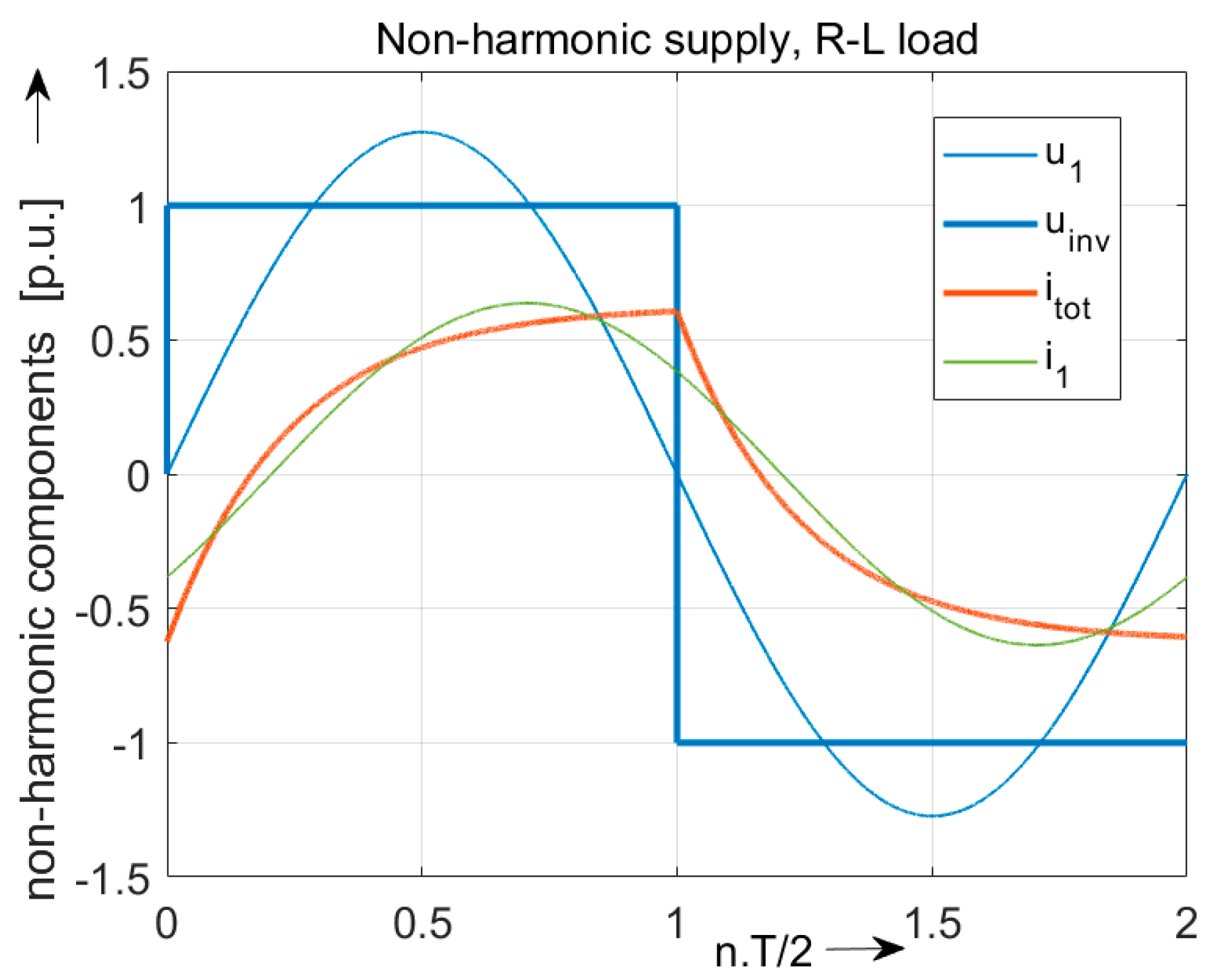
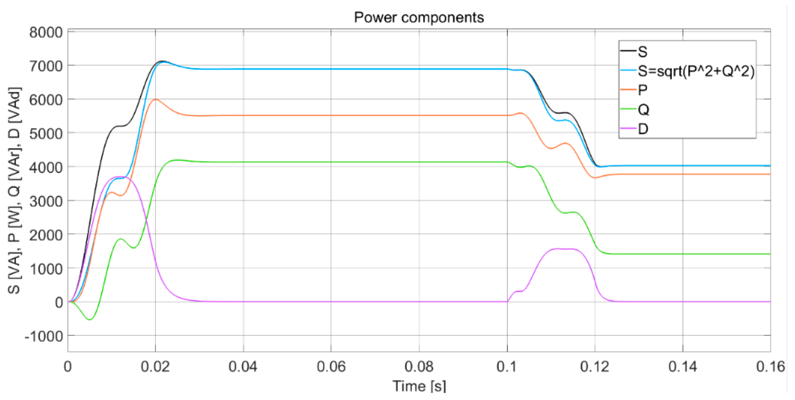
- The determination of the power components’ mean values during transients under the nonharmonic supply and LTI load and under transient conditions caused by a switch-over decreased load;
- -
- The application of the ip-iq method for a three-phase power system under steady and transient states in Matlab/Simulink;
- -
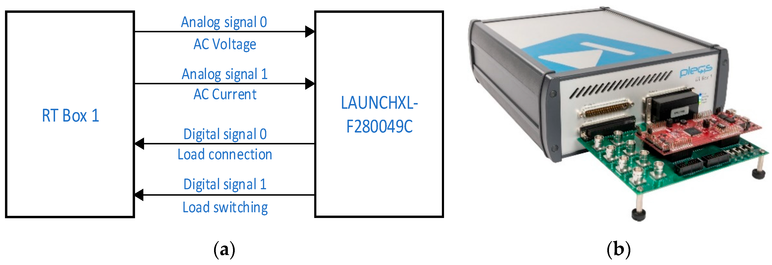
- A modeling and real-time (RT) simulation for single- and three-phase supply systems under different steady and transient conditions using a HIL Simulator Plecs RT Box [19];
- -
- A discussion of each mode of operation, also to time the waveform of each power component during transient, and a conclusion.
2. Ip-Iq Method Used for Apparent, Active, Blind, and Distortion Power Components
- proportional to ,
- proportional to ,
- proportional to (),
- proportional to (),
- and consequently
- as ratio of /,
- THD—as ratio of /,
During Transients
- -
- Using continuous-time filter;
- -
- Using digital filtering;
- -
- Using integral calculus;
- -
- Using a discrete Fourier transform;
- -
- Using artificial neural networks [20].
- (a)
- In the case of harmonic supply and non-harmonic current:
- (b) In the case of non-harmonic supply and quasi-harmonic current:
3. Application of ip-iq Theory on Three-Phase Network and Linear Time-Invariant Load—Simulation Using Matlab/Simulink
- -
- Directly, without any means of interconnection;
- -
- Employing a rectifier (controlled, uncontrolled);
- -
- Employing an inverter (direct, indirect, or cycloconverter).
3.1. Simulation Using Matlab/Simulink
- A.
- Direct connection
3.2. Case of Non-Symmetrical Load
- B.
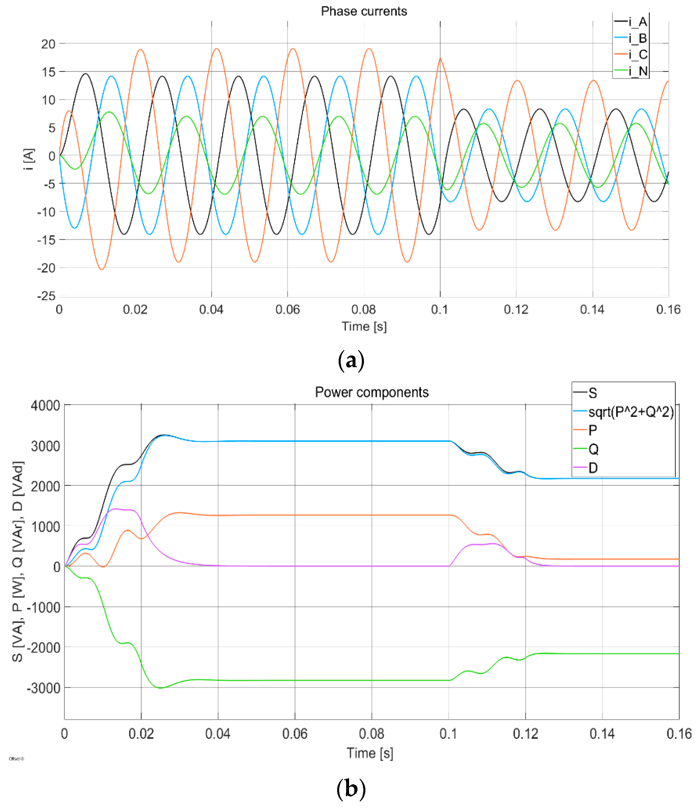
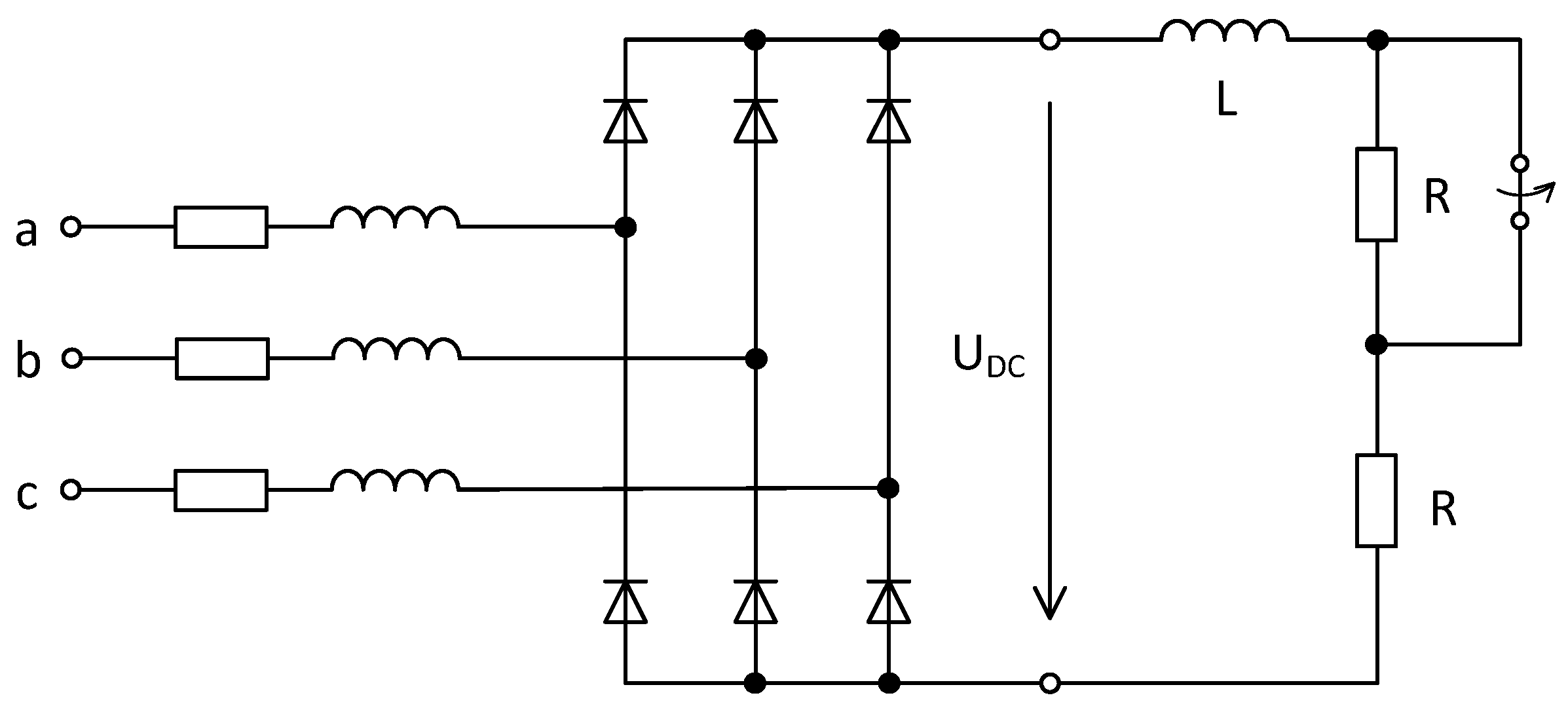
- System with the connection of a diode rectifier
- C.
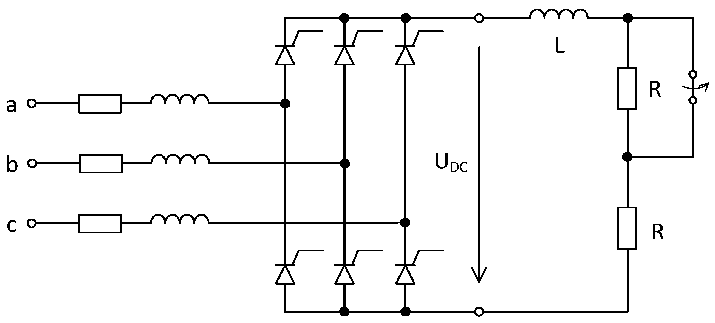
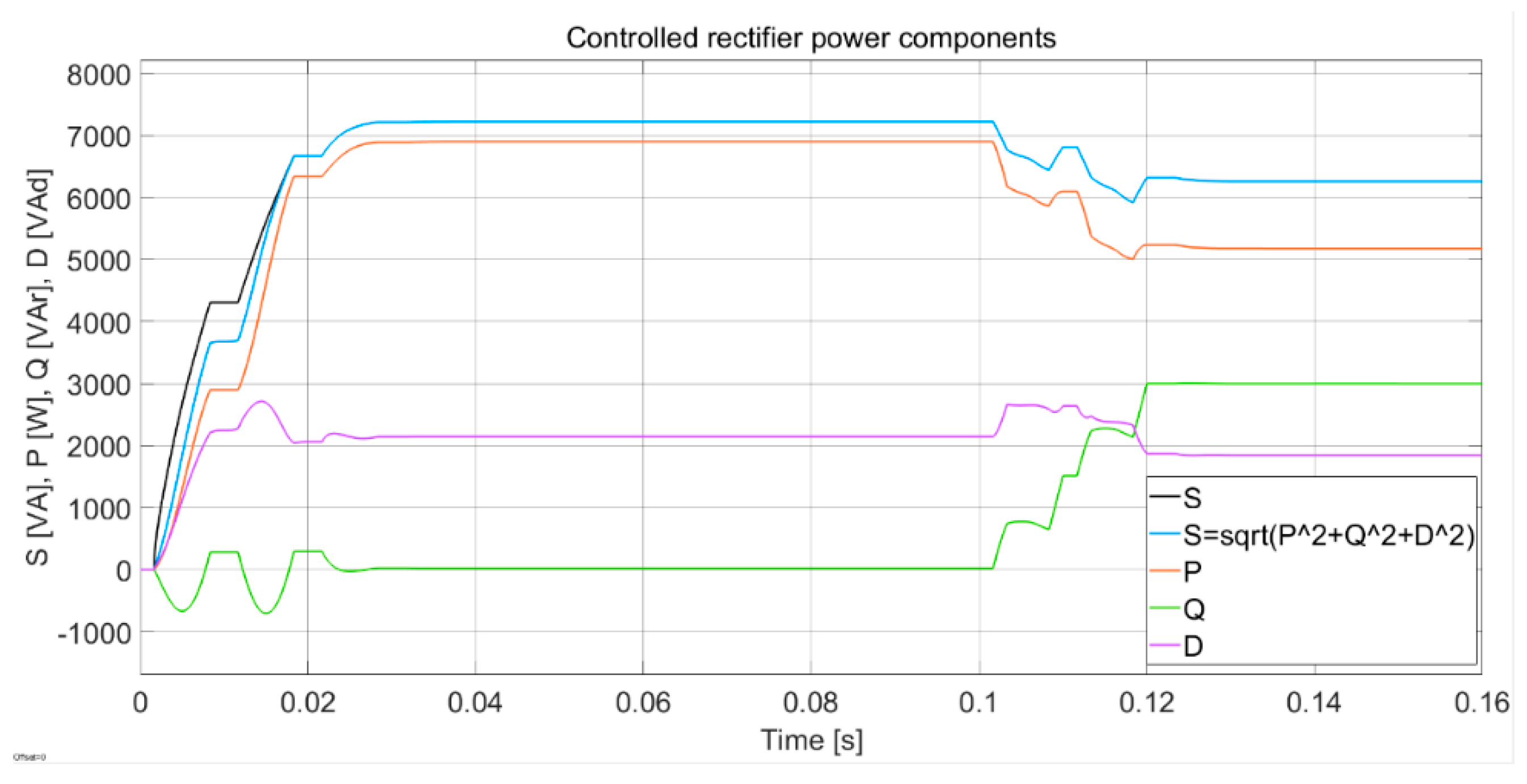
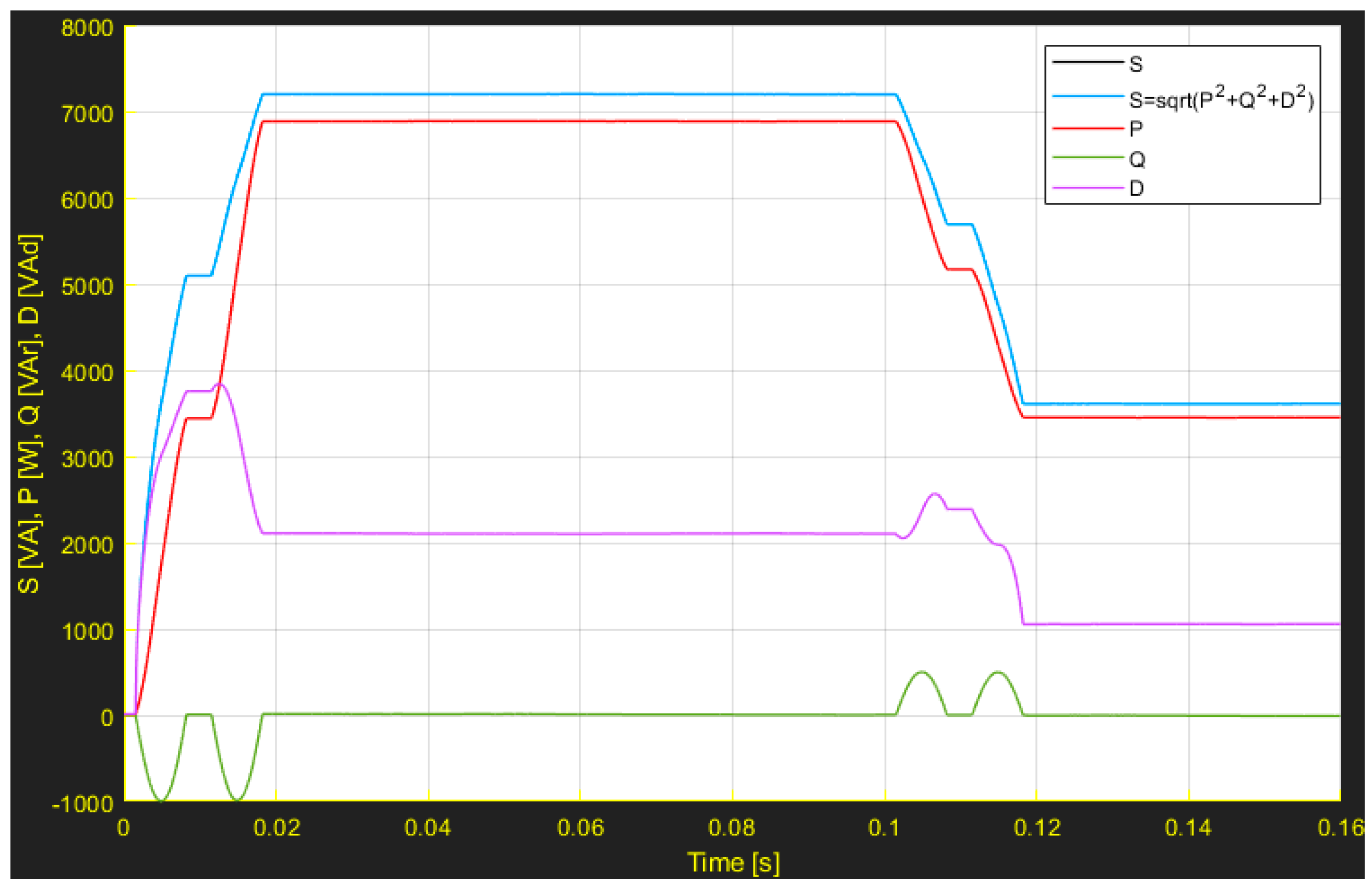
- System with the connection of a controlled rectifier
- D.
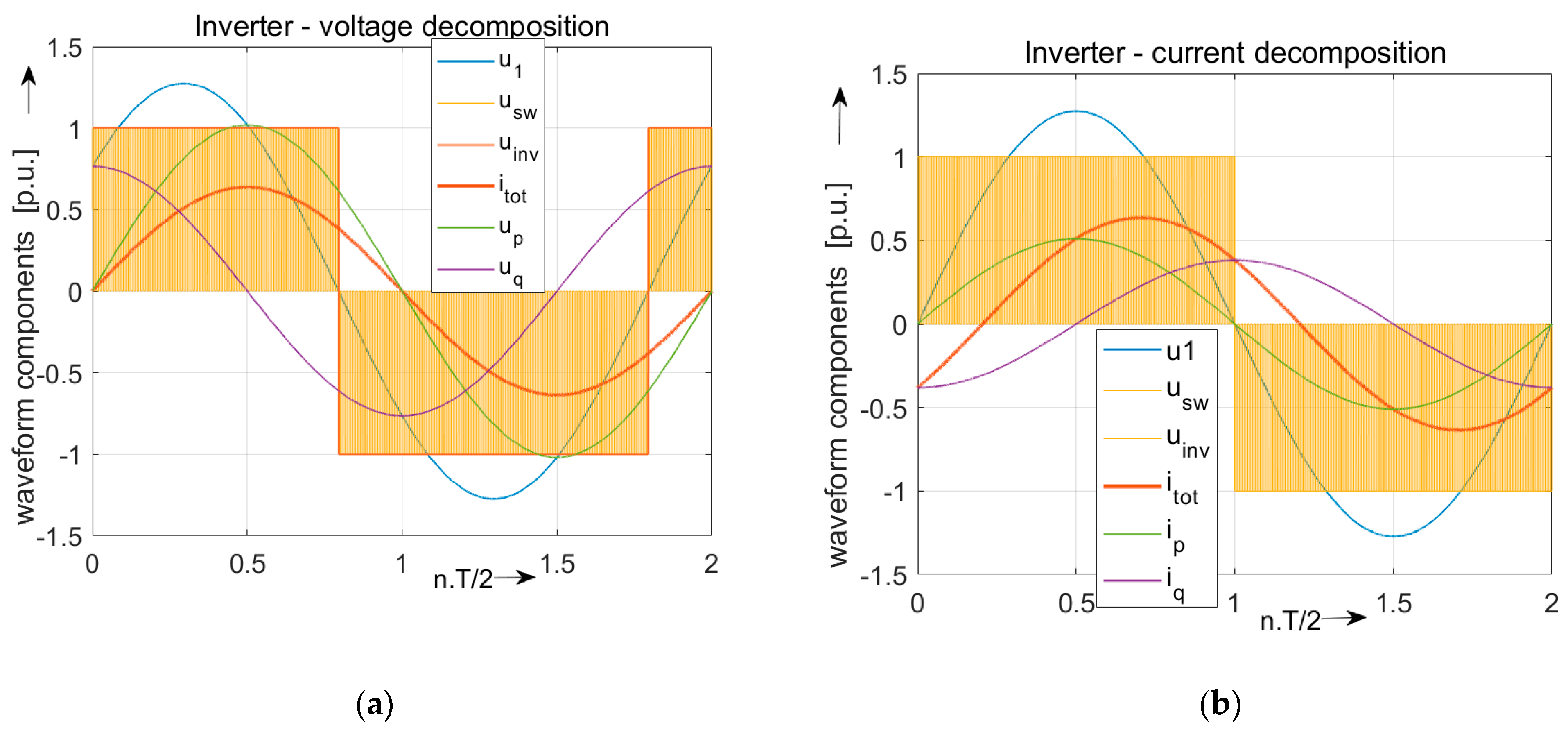
- Three-phase inverter type of VSI and linear RL load
4. Verification of ip-iq Theory by a HIL Simulation (in Real Time)
- A.
- Direct connection of RL load to the network
- B.
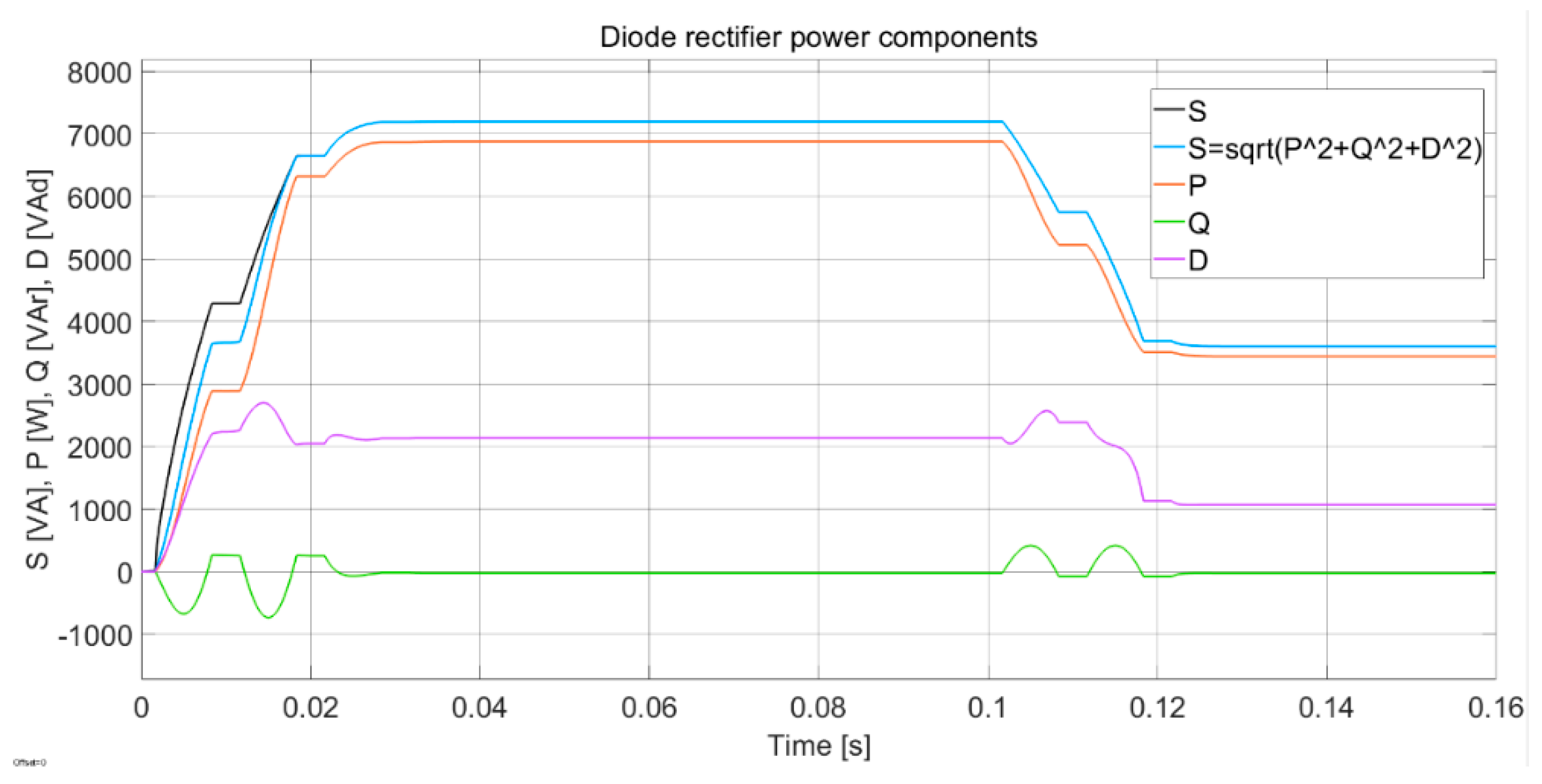
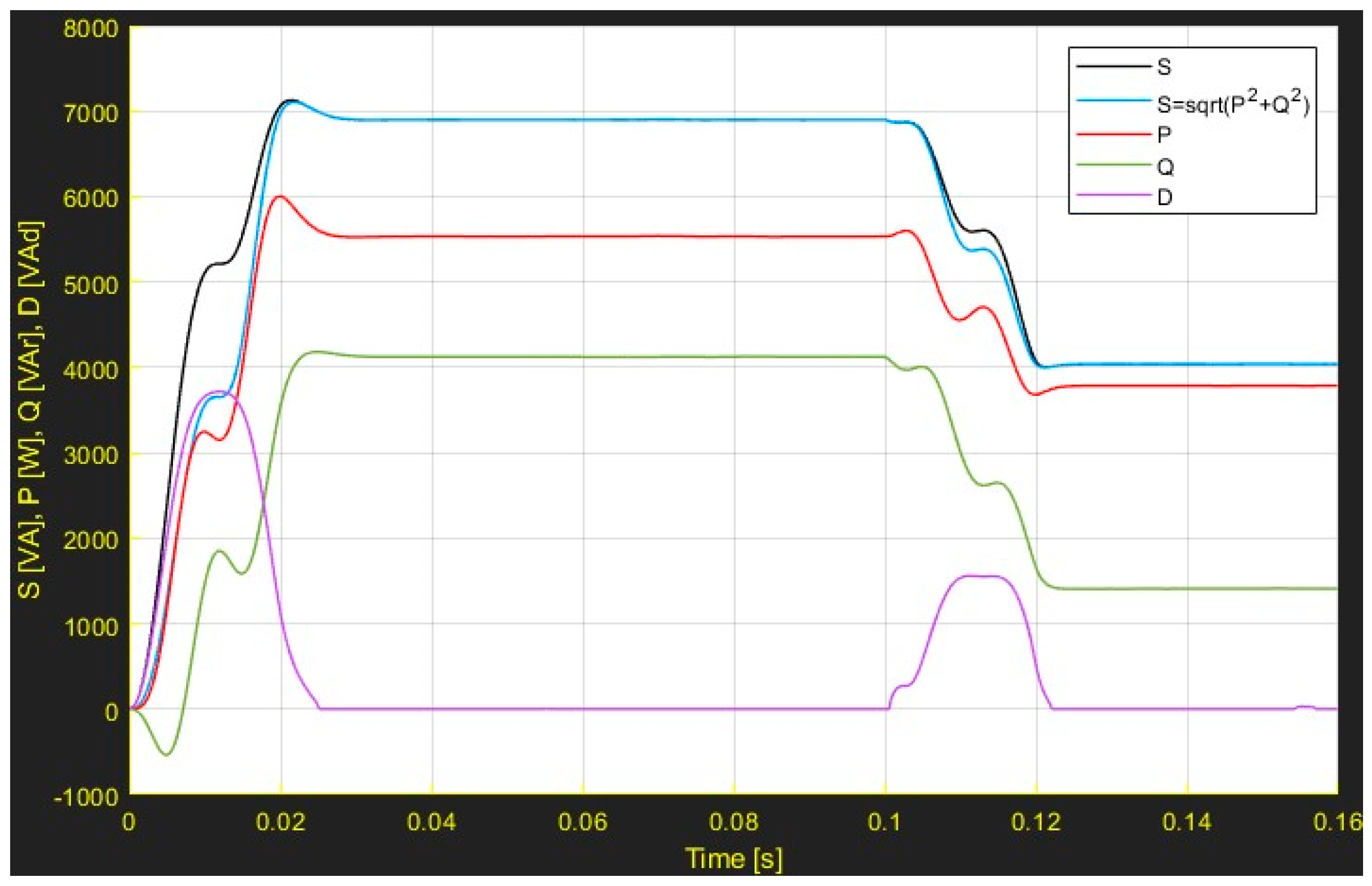
- System with the connection of a diode rectifier
5. Discussion and Conclusions
Author Contributions
Funding
Data Availability Statement
Acknowledgments
Conflicts of Interest
Nomenclature
| PEES | power electrical and electronic systems |
| AVE (ave) | average value or function |
| RMS (rms) | root mean square value or function |
| N | number of sliding window points |
| Clarke transformation constant | |
| p-q | instantaneous active and reactive power method |
| ip-iq | instantaneous active and reactive power method |
| , | instantaneous active and reactive power components |
| phase voltages in -coordinate system | |
| phase currents in -coordinate system | |
| the amplitude of phase current | |
| apparent power | |
| active power | |
| reactive blind power | |
| reactive distortion power | |
| power factor | |
| THD | total harmonic distortion |
| active power of fundamental harmonic | |
| active power of a zero-sequence component | |
| discretized power components at - time instants | |
| components of a non-symmetrical system in - coordinates | |
| components in - coordinates | |
| voltage and current zero-sequence power components | |
| neutral wire current | |
| ihh(t) | sum of high harmonics |
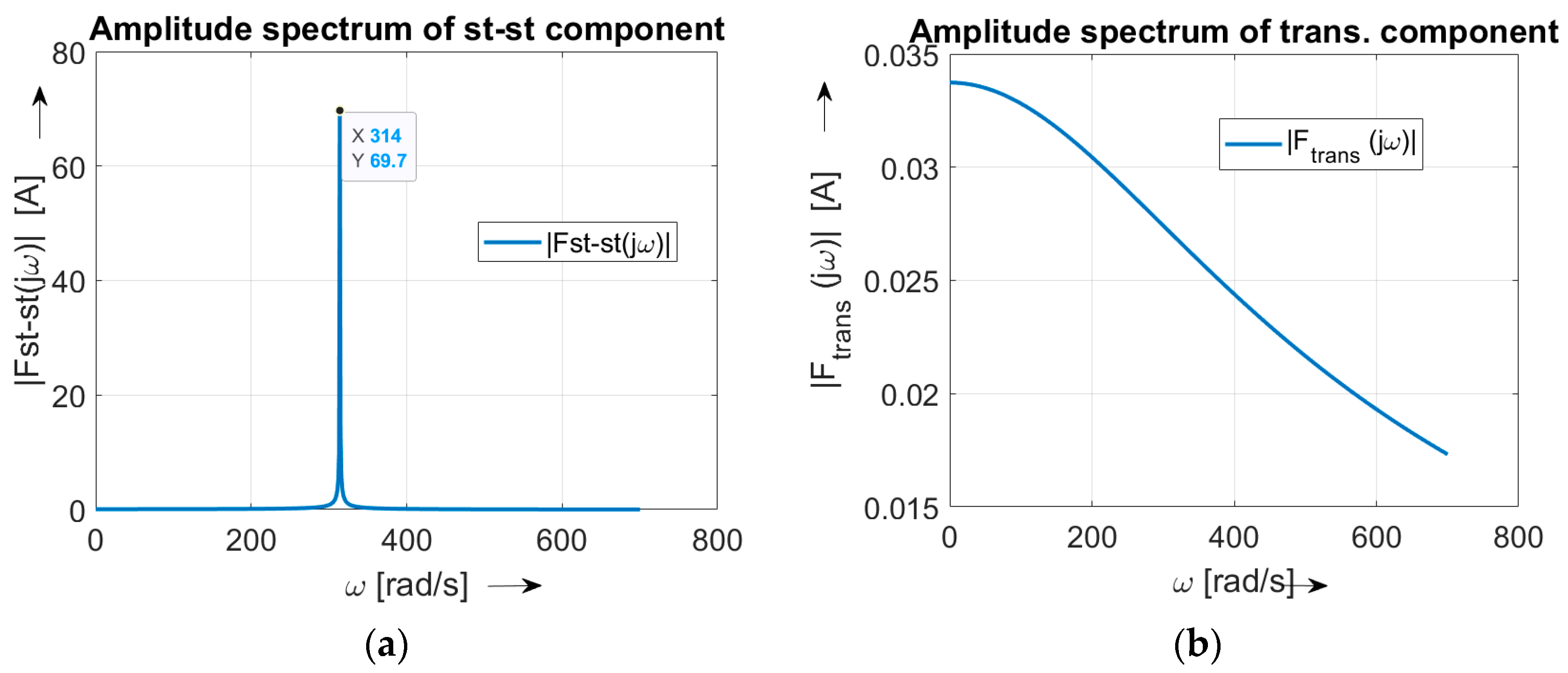
| ist-st | steady-state current component |
| , , | phase shift, PF of fundamental harmonic |
| impedance, resistance, and inductance of the load |
References
- Akagi, H.; Kanazawa, Y.; Nabae, A. Generalized Theory of the Instantaneous Reactive Power in Three-Phase Circuits. In Proceedings of the IPEC Conference, Tokyo, Japan, 27–31 March 1983; pp. 1375–1386. [Google Scholar]
- Czarnecki, L.S. Currents’ Physical Components (CPC) Concept: A Fundamental of Power Theory. In Proceedings of the International School on Non-sinusoidal Currents and Compensation, Lagow, Poland, 10–13 June 2008; pp. 1–11. [Google Scholar]
- Guo, J.; Xiao, X.N.; Tao, S. Discussion on Instantaneous Reactive Power Theory and Current Physical Component (CPC) Theory. In Proceedings of the 15th International Conference on Harmonics and Quality of Power, Hong Kong, China, 17–20 June 2012; pp. 427–432. [Google Scholar] [CrossRef]
- Dugan, R.C.; McGranaghan, M.F.; Santoso, S.; Beaty, H.W. Electrical Power Systems Quality, 2nd ed.; McGrow-Hill Copyrighted Material; McGraw Hill: Maidenhead, UK, 2004. [Google Scholar]
- Kryltcov, S.; Makhovikov, A.; Korobitcyna, M. Novel Approach to Collect and Process Power Quality Data in Medium-Voltage Distribution Grids. Symmetry 2021, 13, 460. [Google Scholar] [CrossRef]
- Varga, L.; Hlubeň, D. Measuring Methods in Electro-Energetics; Technical University Košice: Košice, Slovakia, 2002; 175p, Chapter 1; pp. 15–21. (In Slovak) [Google Scholar]
- Kouzou, A.; Ismeil, M.A.; Abu Rub, H.; Ahmed, S.M.; Mahmoudi, M.O.; Boucherit, M.S.; Kennel, R. Discussions on the Instantaneous Reactive Power Theory Terms in the General Case Based on the Symmetric Components. In Proceedings of the International Conference on Renewable Energies and Power Quality (ICREPQ’12), Santiago de Compostela, Spain, 28–30 March 2012. [Google Scholar]
- Dobrucký, B.; Koňarik, R.; Beňová, M.; Praženica, M. A New Modified Non-Approximative Method for Dynamic Systems Direct Calculation. Appl. Sci. 2023, 13, 4162. [Google Scholar] [CrossRef]
- Shenkman, A.L. Transient analysis using the Fourier transform. In Transient Analysis of Electric Power Circuits Handbook; Springer: Dordrecht, The Netherlands, 2005; Chapter 4; pp. 213–263. ISBN -10 0-387-28799-X. [Google Scholar]
- Bai, H.; Mi, C. Transients of Modern Power Electronics; John Wiley & Sons, Ltd.: Chichester, UK, 2011; ISBN 978-0-470-68664-5. [Google Scholar]
- Peretyatko, L.; Spinul, L.; Shcherba, M. Theoretical Fundamentals of Electrical Engineering, Part I; IS Polytechnic Institute: Kiev, Ukraine, 2021; Chapters 5–6; pp. 36–54. [Google Scholar]
- Kreyszig, E.; Kreyszig, H.; Norminton, E.J. Advanced Engineering Mathematics; John Wiley & Sons, Inc.: New York, NY, USA, 2011; Chapter 6; pp. 203–255. ISBN 978-0-470-45836-5. [Google Scholar]
- Mohan, N.; Undeland, T.M.; Robbins, W.P. Power Electronics: Converters, Applications, and Design, 3rd ed.; John Wiley & Sons, Inc.: New York, NY, USA, 2003. [Google Scholar]
- Hartman, M.T. Why the new physical interpretations of the reactive power on terms of the CPC power theory is not true? In Proceedings of the International Conference CPE ‘07on Compatibility in Power Electronics, Gdansk, Poland, 29 May–1 June 2007. [Google Scholar] [CrossRef]
- Czarnecki, L.S. Physical Phenomena that Affect the Effectiveness of the Energy Transfer in Electrical Systems. In Proceedings of the 20th International Scientific Conference on Electric Power Engineering (EPE), Kouty nad Desnou, Czech Republic, 15–17 May 2019. [Google Scholar] [CrossRef]
- Herrera, R.S.; Salmerón, P. Present point of view about the instantaneous reactive power theory. IET Power Electron. 2009, 2, 484–495. [Google Scholar] [CrossRef]
- Soares, V.; Verdelho, P.; Marques, G.D. An instantaneous active and reactive current component method for active filters. IEEE Trans. Power Electron 2000, 15, 660–669. [Google Scholar] [CrossRef]
- Verdelho, P.C. Voltage type reversible rectifiers control methods in unbalanced and nonsinusoidal conditions. In Proceedings of the IECON 98—24th Annual Conference of the IEEE Industrial Electronics Society, Aachen, Germany, 31 August–4 September 1998. [Google Scholar] [CrossRef]
- Plexim. A HIL Simulator on Every Engineer’s Desk. Available online: https://www.plexim.com/products/rt_box/rt_box_1 (accessed on 26 March 2024).
- Osowski, S. Neural network for estimation of harmonic components in a power system. IEE Proc. GTD 1992, 139, 129–135. [Google Scholar] [CrossRef]


| Load | ] | ] | ] | ] | |||
|---|---|---|---|---|---|---|---|
| before | 43.94 | ||||||
| after |
| Load | ] | ] | ] | ] | |||
| before | |||||||
| after | 0.82 | ||||||
| Simulation results before and after change (at steady states) | |||||||
| Time | |||||||
| Load | ] | ] | α [deg} |
|---|---|---|---|
| before | 41.91 | 100 | 0 |
| after | 83.82 | 100 | 0 |
| Load | ] | ] | α [deg} |
|---|---|---|---|
| before | 41.91 | 100 | 0 |
| after | 41.91 | 100 | 30 |
| Load | ] | ] | ] | ] | |||
|---|---|---|---|---|---|---|---|
| before | 16.58 | 4.775 | 56.31 | 0.550 | 0.835 | ||
| after | 23.00 | 2.387 | 37.87 | 0.797 | 0.604 |
Disclaimer/Publisher’s Note: The statements, opinions and data contained in all publications are solely those of the individual author(s) and contributor(s) and not of MDPI and/or the editor(s). MDPI and/or the editor(s) disclaim responsibility for any injury to people or property resulting from any ideas, methods, instructions or products referred to in the content. |
© 2024 by the authors. Licensee MDPI, Basel, Switzerland. This article is an open access article distributed under the terms and conditions of the Creative Commons Attribution (CC BY) license (https://creativecommons.org/licenses/by/4.0/).
Share and Cite
Dobrucký, B.; Kaščák, S.; Šedo, J. Power Components Mean Values Determination Using New Ip-Iq Method for Transients. Energies 2024, 17, 2720. https://doi.org/10.3390/en17112720
Dobrucký B, Kaščák S, Šedo J. Power Components Mean Values Determination Using New Ip-Iq Method for Transients. Energies. 2024; 17(11):2720. https://doi.org/10.3390/en17112720
Chicago/Turabian StyleDobrucký, Branislav, Slavomír Kaščák, and Jozef Šedo. 2024. "Power Components Mean Values Determination Using New Ip-Iq Method for Transients" Energies 17, no. 11: 2720. https://doi.org/10.3390/en17112720
APA StyleDobrucký, B., Kaščák, S., & Šedo, J. (2024). Power Components Mean Values Determination Using New Ip-Iq Method for Transients. Energies, 17(11), 2720. https://doi.org/10.3390/en17112720