Abstract
Growing dependence on fossil fuels is one of the critical factors accelerating climate change, a global concern that can destabilize ecosystems and economies worldwide. In this context, renewable energy is emerging as a sustainable and environmentally responsible alternative. Among the options, geothermal energy stands out for its ability to provide heat and electricity consistently and efficiently, offering a feasible solution to reduce the carbon footprint and promote more sustainable development in a globalized economy. In this work, a machine learning approach is proposed to predict the behavior of a horizontal heat exchanger from a bioclimatic house. First, a correlation analysis was conducted for optimal feature selection. Then, several regression techniques were applied to predict the output temperature of the geothermal exchanger. Satisfactory prediction results were obtained in different scenarios over the whole dataset. Also, a significant correlation between several sensors was concluded.
1. Introduction
In the last decades, climate change, global economic instability, and increasing dependence on fossil fuels have become urgent challenges requiring an accelerated transition to more sustainable and efficient energy sources [1]. In this context, renewable energy, including geothermal energy, emerges as a promising alternative to provide a clean and constant energy supply [2]. Unlike solar and wind energy, whose technologies have evolved significantly due to their popularity, geothermal energy still requires technological development and more efficient implementation [3], primarily in areas with suitable geological conditions.
Geothermal energy is described as energy stored as heat beneath the ground inside the earth [4]. According to several studies, the earth’s total heat emitted is around 42 × 1012 W [4]. Only 2% of this energy is present at the crust; the other 82% corresponds to the mantle due to the decomposition of several radioactive isotopes, and the remainder comes from the core. Despite the large amount of available energy, its utilization is limited to areas with specific geological conditions [5].
In recent decades, technological advances have allowed for greater efficiency in geothermal heat extraction, reducing costs and expanding the geographic potential of this source [6]. In addition, the focus on sustainability and reducing dependence on fossil fuels has led several governments to increase investment in geothermal research and development [7].
Regarding electricity generation, geothermal energy’s total installed capacity in the twenty-first century’s first decades was nearly 9 MW. Nevertheless, the power associated with non-electrical uses was approximately 15 MW. In this sense, non-electrical applications involve space heating, greenhouses, aquaculture, industrial activities, or heat pumps, among others [4].
Among geothermal solutions, ground source heat exchangers, which take advantage of the more stable subsurface temperature, are particularly promising for residential and commercial applications [8]. This study focuses on a horizontal geothermal configuration implemented in a bioclimatic house.
Horizontal heat exchanger geothermal energy systems harness the thermal energy stored below the earth’s surface to provide efficient heating and cooling [9]. These systems are mainly composed of pipes arranged horizontally at a relatively shallow depth, usually between 1 and 2 m [10]. Although horizontal configurations are less expensive than vertical configurations [11], their efficiency can be affected by seasonal thermal variability, which poses significant challenges in terms of energy efficiency [12].
Different works focus on the importance of predicting thermal resistance or soil temperature in geothermal systems [13,14]. On the other hand, in ref. [15], a fault detection and recovery approach is proposed to identify a malfunctioning sensor on a geothermal system. More specifically, artificial neural network (ANN)-based methods [16,17] or random forest techniques [18] were applied to predict the performance of a geothermal heat pump system. Also, ref. [19] develops a performance prediction model of an air-cooled heat pump system using ANN, support vector machine (SVM), random forest (RF), and K-nearest neighbor (KNN). In this sense, ref. [20] proposes linear regression, nonlinear regression, and ANN techniques to predict the influence of the input variables on the heat transfer rate and heat transfer rate variation of a ground source heat pump (GSHP). In addition, ref. [21] develops a method for predicting the behavior of a horizontal geothermal heat exchanger by means of several time series techniques.
As stated above, several approaches have been proposed for predicting the behavior of GSHPs or geothermal heat exchangers. Nevertheless, there is not extensive work focused on bioclimatic housing involving several renewable energy sources. In this sense, this research deals with a multi-energy context including wind power, solar thermal, solar photovoltaic, biomass, and geothermal energy systems. This is important to ensure an efficient system management and optimize the energy demand. Moreover, no published work in this context involves the use of the intelligent techniques proposed for this study.
The present research proposes a method based on intelligent regression techniques to predict the output temperature of a geothermal heat exchanger using the input temperature and the ground reference temperature as predictors. The exchanger includes these sensors and several buried temperature sensors throughout its length. One of the reasons for installing these buried sensors is to detect possible obstructions along the path. In this sense, this approach aims not only to optimize the thermal performance of the system and its energy demand but also to improve sensor maintenance, avoiding costly and time-consuming interventions.
In general terms, this study aims to promote more accessible housing by reducing the costs of sensor installation in difficult-to-access locations. It should be noted that the replacement of a buried probe can be expensive. In addition, the optimization of renewable energy systems by means of artificial intelligence (AI) techniques contributes to the reduction of greenhouse gas emissions. Furthermore, this work seeks to improve the performance of the methods used in previous work.
Satisfactory results were obtained by applying several machine learning (ML) techniques, achieving a good prediction of the output temperature of the heat exchanger. Specifically, recursive least square, K-nearest neighbors, decision tree, random forest, polynomial regression, support vector regression, and multilayer perceptron techniques were proposed for this study. In addition, several metrics were proposed for an in-depth model evaluation. Furthermore, a statistical analysis was carried out to determine which of the techniques provided the best results. Furthermore, this study has evidenced a significant correlation between different sensors of the geothermal system.
This paper is structured as follows. After the present introduction, a brief description of the case of study is presented. Then, the methods section is exposed. Subsequently, experiments and results are shown in the following section, and, finally, conclusions and future work are presented.
2. Case of Study
This section describes the geothermal system under study, located in a bioclimatic house, and the dataset obtained from periodical sensor measurements.
2.1. Sotavento Bioclimatic House
The bioclimatic house analyzed results from a project developed by the Sotavento Galicia Foundation, which aims to demonstrate the viability of different renewable systems and promote their use. This house is located in the Sotavento Experimental Wind Farm facilities between the municipalities of Xermade (Lugo) and Monfero (A Coruña) in the autonomous community of Galicia, Spain. Its geographical coordinates are 43°21′ North, 7°52′ West. It is located at an altitude of 640 m and 30 km from the sea.
The bioclimatic house’s thermal and electrical installations are supported by several types of renewable energy systems. Wind turbines and photovoltaic panels generate electricity. Furthermore, when these energy sources are insufficient to meet demand, the power grid supplies electricity to the home’s lighting and power systems. In contrast, the thermal installation manages the charge of the heating system and domestic hot water (DHW). Solar, geothermal, and biomass energies serve to carry out this task.
The thermal installation is divided into three main sections: generation, accumulation, and consumption.
Generation: The generation system is composed of three renewable energy sources:
- Solar thermal system: The solar panels absorb energy from the solar radiation and heat the fluid of the primary circuit. Then, this fluid is fed into a solar accumulator.
- Biomass boiler system: a biomass boiler with a pellet yield of 90% provides hot water to the inertial accumulator, ensuring an internal temperature of around 63 °C.
- Geothermal system: It combines a ground source heat pump and a horizontal heat exchanger. The heat exchanger consists of several pipes arranged horizontally at depth of 2 m. The warm water from the heat pump is driven directly to the inertial accumulator.
Accumulation: this group comprises two accumulation units: a solar accumulator and an inertial accumulator for heat supply and DHW. A preheating system is also integrated to reach the temperature setpoint if necessary.
Consumption: The inertial accumulator supplies DHW and underfloor heating. The DHW supplies the bathroom and kitchen, dimensioning the system according to the Spanish Technical Building Code (240 L per day). The underfloor heating system keeps the house temperature between 18° C and 22 °C. For this purpose, the water temperature is regulated between 35 °C and 40 °C.
As stated in the Introduction section, this paper focuses on the geothermal energy system described in depth in the following subsection.
2.2. Geothermal Heat Pump and Horizontal Heat Exchanger
As stated above, heat generation through a horizontal heat exchanger is among the proposed active solutions. Figure 1 shows the topology of the geothermal system, involving both heat pump (AT2) and horizontal heat exchanger. In this case, two circuits are connected to the heat pump: the primary circuit, including the heat exchanger (the circuit of the right side including S28 and S29 temperature sensors), and the second circuit (left side including S30 and S31 temperature sensors and a flowmeter C6), connecting the heat pump to the inertial accumulator.
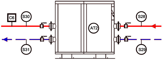
Figure 1.
Geothermal heat pump system scheme.
Figure 2 shows a simplified scheme of the horizontal heat exchanger. The geothermal heat exchanger is composed of four parallel circuits with a total length of 100 m per circuit. Eight sensors (S3xx) are located along each circuit to measure the ground temperature in different positions while the system operates. Also, a reference sensor (S401) is used to monitor the ground temperature. Furthermore, the system includes input (S28 in Figure 1) and output (S29 in Figure 1) temperature sensors for the geothermal heat exchanger. Finally, a thermal power sensor is located at the second circuit of the heat pump.
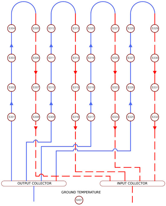
Figure 2.
Horizontal heat exchanger scheme.
2.3. Dataset Description
A sensor data acquisition over a 1 year period has been performed. It should be noted that parallel circuit sensor data are only available for one of the four circuits. In this sense, the dataset comprises a total of 52,645 observations with a sampling rate of 10 min. The features that compose the dataset are described below:
- date-time (yyyy-mm-dd hh:mm): date-time for the corresponding observation.
- Tin (°C): return temperature of the horizontal heat exchanger circuit to the heat pump.
- Tout (°C): output temperature from the heat pump to the heat exchanger circuit.
- Tref (°C): reference temperature of the ground.
- c1sn (°C): temperature sensor n for horizontal heat exchanger circuit 1.
- Pavg (W): output thermal power of the heat pump, averaged over 10 min.
2.4. Data Preparation
First, a data exploration stage was performed where several observations were discarded due to missing data. Then, from the initial 52,645 samples, the resulting number of samples is reduced to 52,638. Next, the samples where the heat pump was turned off, resulting in an output thermal power, or Pavg, of 0 W, were eliminated, yielding a dataset of 4883 samples. Then, the date-time feature was removed from the dataset. Finally, a standardization was applied to the dataset, giving a mean value of 0 and a variance of 1.
3. Methods
The following subsections describe the methods applied in this study.
3.1. Correlation Analysis
A correlation analysis was performed to optimize feature selection for model fitting. For this purpose, a correlation matrix is obtained from all dataset features. A correlation matrix is a statistical study that can determine the strength and direction of linear relationships between variables. It represents the correlations between pairs of variables in a symmetric square matrix [22]. The correlation values are expressed using numbers ranging from −1 to 1. Values approaching zero indicate no linear correlation. Numbers near 1 suggest a positive, intense connection, whereas numbers near −1 imply negative, strong correlations.
3.2. Regression Techniques
The regression techniques used for this study are exposed in the following subsections.
3.2.1. Recursive Least Squares Regressor
The recursive least squares (RLS) algorithm minimizes the sum of squared errors, which are the differences between predictions and actual values [23]. This technique uses a linear function to model the relationship between target y and features X, using model parameters w. This relationship can be expressed through Equation (1), with n being the number of features.
3.2.2. K-Nearest Neighbors
K-nearest neighbors (KNN) is a well-known supervised non-linear algorithm [24,25]. When used in a regression setting, it predicts the input data value given the mean of its K nearest neighbors of the training data. During the training stage, KNN does not build any model but stores the training data. The algorithm can be appropriately tuned by modifying the number of neighbors, K and the weighting scheme for each neighbor.
3.2.3. Decision Tree Regressor
The decision tree (DT) algorithm is a non-parametric technique [26] that employs a tree diagram to divide the data into more homogeneous and smaller groups at each node. When the trained model reaches the final node, it predicts a numerical value. For this purpose, the model uses if–then conditions from learned rules based on the explanatory variables. Additionally, the model can be tuned to improve its performance by choosing the criteria for the maximum tree depth and the best data split for each node.
3.2.4. Random Forest Regressor
In contrast to DT, the random forest (RF) technique groups various decision trees to build the final model [27]. With the aim of obtaining different regressors, each single decision tree is trained with slightly different datasets. In this sense, the model’s final prediction is an average of the results of each tree.
Several hyperparameters can be used for model tuning. For instance, the maximum depth and the criteria of the tree diagram, the number of regressors used to implement the forest, and some specific configurations for the decision trees.
3.2.5. Polynomial Regression
Polynomial regression (PN) is a type of linear regression in which the relationship between the independent variables and the dependent variable is modeled as polynomials of degree n [28]. Like linear regression, it permits the restriction of coefficients to non-negative values and includes the option to fit an intercept term—additionally, the highest degree of the polynomial acts as a hyperparameter.
3.2.6. Support Vector Regression
The support vector regression (SVR) technique is a support vector machine (SVM) variant used for regression tasks [29]. This generalized version adds an insensitive region wrapping the decision function of the SVM (-tube), allowing the model to return a continuous output to be applied in regression problems. Among the configurations for the algorithm are the regularization parameter and the kernel type, which modifies the decision function and maps the input data into other dimensional space.
This modification generalized the classification problem, adding an insensitive region wrapping the decision function of the SVM, called -tube, which allows the model to return a continuous output to resolve regression problems. It is possible to set, as well as the -tube, the kernel type used in the algorithm, which modifies the decision function and maps the input data into other dimensional space, and the regularization parameter.
3.2.7. Multilayer Perceptron
The multilayer perceptron (MLP) is an artificial neural network composed of multiple neuron layers, each connected to the others by weighted synapses [30]. A typical MLP structure includes an input layer, one or more hidden layers, and an output layer. The neurons from the hidden and output layers generally use non-linear activation functions, such as the sigmoid function or hyperbolic tangent. The number of neurons for each layer is selected individually: the input layer has as many neurons as the number of features, the output layer has the same number of neurons as predicted values, and an arbitrary number of neurons is selected for the hidden layers.
In this feedforward network, the data flow from the input to the output layer and can be used for regression and classification. The learning process of an MLP is based on the backpropagation algorithm. In this sense, the error between the predicted value and the actual value is computed and used to update the weights of the connections within the network.
3.3. Statistical Analysis
With the aim of selecting the best model, a statistical analysis was conducted to determine which regression technique achieves significantly better results. In this sense, two different tests were executed: the Kruskal–Wallis H-test and the Tukey test.
The Kruskal–Wallis H-test is a non-parametrical test [31] that determines if significant differences exist between the median of independent groups’ data by evaluating the null hypothesis that the medians are equal. The Kruskal–Wallis H-test returns the p-value, a statistical measure to determine the probability that a computed statistical value is possible given a true null hypothesis. A significance level is used as a threshold to determine if the p-value is statistically significant. The null hypothesis is rejected if the p-value is less than or equal to . In this case, the data groups differ.
Tukey’s honestly significant difference (HSD) test [32] performs a pairwise comparison to accept or reject the null hypothesis between two groups. This test also needs a proper adjustment of the significance level, .
4. Experiments and Results
The experiments setup and their results are detailed below.
4.1. Experiment Setup
In this subsection, the tools used in this research are presented. The different tested configurations of the regression techniques, as well as the metrics used to evaluate and compare the performance of the models, are mentioned below.
Figure 3 shows the process followed in the present research for model building. The result is a validated model capable of predicting the output temperature of the geothermal heat exchanger.

Figure 3.
Model building process flowchart.
4.1.1. Regression Techniques
Different techniques’ configurations are tested to obtain the best models. Below are the hyperparameters and values tested.
Recursive Least Squares Regressor
The model configuration affects the application of the independent term, which may be computed or set to zero, as well as the coefficients’ sign, which can be constrained to be positive. Consequently, this leads to four distinct models.
K-Nearest Neighbors
Various numbers of neighbors were tested to make the prediction, ranging from 1 to 41, in a 4-step number. Additionally, two methods for assigning the model’s weight distribution were employed: a uniform function, which gives equal weight to all neighbors, and a distance function, which assigns a weight to a neighbor that is inversely proportional to its distance from the query point. This resulted in a total of twenty-two distinct models.
Decision Tree Regressor
The diagram’s maximum depth was set from 1 to 10, incrementing by 1. Additionally, various criteria for splitting were applied based on both absolute and squared errors, resulting in twenty distinct models.
Random Forest Regressor
The identical hyperparameters and values assessed in decision tree models were applied, including the number of regressors (trees) utilized by the model, evaluating two, three, four, five, and six trees, yielding one hundred distinct models.
Polynomial Regression
Several polynomial equations were tested in order to enhance the prediction’s quality, using a polynomial from the second degree to one of the tenth degree. The constant term was either computed or set to zero to fine-tune the regression. In total, eighteen distinct models were evaluated.
Support Vector Regression
The modified hyperparameters include the regularization coefficient, epsilon, and kernel function. The first two were varied between 10, 1, 0.1, 0.01, and 0.001, while the kernel function was tested with four different types: linear, sigmoid, radial basis function (RBF), and a two- and three-degree polynomial. Consequently, this led to the creation of one hundred twenty-five distinct models.
Multilayer Perceptron
The MLPs were trained using a batch size of 32 samples over 200 epochs. They were designed with a single hidden layer, and the output layer’s activation function was linear. The count of hidden neurons tested ranged incrementally from one to twenty neurons in a step of one neuron. The activation functions employed were rectified linear unit (ReLU), sigmoid, and hyperbolic tangent, culminating in sixty configurations.
4.1.2. Model Evaluation
Different metrics were used throughout the development of this research. All metrics are found in Table 1. Lower mean squared error and mean absolute error values mean good model performance, whereas symmetric mean absolute percentage error yields a range from 0 to 200%, with 0% representing the ideal case. For the coefficient of determination, values approaching 1 denote favorable model behavior, while values close to 0 indicate poor performance.

Table 1.
Employed evaluation metrics.
The evaluation of these metrics occurs in two stages. Initially, a comparison is made from the metrics results of a 10-fold cross-validation conducted on 80% of the data samples, reserving the remaining samples to the testing phase. After identifying the optimal model configuration, the model is trained with that 80% (the first stage complete dataset). Then, the remaining 20% of the samples is utilized in the testing phase to evaluate the model’s generalization and to validate the model’s performance. This 20% corresponds to new observations or samples that have not been previously seen.
Following the initial step, a Kruskal–Wallis H-test will be conducted to determine if there are significant differences in the performance of the models. Tukey’s HSD test will be carried out if the null hypothesis is rejected. This research has set a significance level of 5% ().
4.2. Results
This subsection presents the different results obtained in the correlation analysis, model configuration selection, training phase, and validation phase.
4.2.1. Correlation Analysis
Figure 4 displays the correlation matrix for the variables measured within the geothermal system. One notable observation is the significant correlation value among the temperature sensors for the horizontal heat exchanger, c1sn, which can be attributed to their proximity and identical terrain conditions. Consequently, the ground reference temperature, Tref, exhibits a high correlation with these sensors. As the primary goal of this research is to obviate the need for horizontal sensors, they will not be utilized in the study.
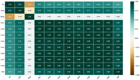
Figure 4.
Correlation matrix of the dataset variables.
The average output thermal power of the heat pump, Pavg, does not demonstrate a linear correlation with most variables, except for the Tin sensor. A substantial correlation is observed between the temperature sensors of the heat exchanger, Tin and Tout.
4.2.2. Regression Techniques Results
Table 2 shows the configuration that obtained the best values in the metrics for each regression technique during the cross-validation phase.

Table 2.
Model hyperparameters with best performance.
The independent term is calculated automatically in the RLS technique, and the coefficient is not forced to be positive. For the KNN algorithm, a number of 13 neighbors is used, and the weight function is uniform. In the case of the DT, the maximum depth of the diagram is six, and the criterion used is the squared error. For the RF, six trees are used, the maximum depth of the diagram is seven, and the criterion is also the squared error. In the polynomial (PN) technique, the degree is set at 7, and the constant term is determined automatically. A radial basis function kernel, a regularization coefficient of 10, and an epsilon of 0.1 are used for SVR. Finally, in the MLP, 15 hidden neurons are used, and the activation function is the sigmoid.
MSE, MAE, SMAPE, and average values along all folds in the cross-validation phase are represented in Table 3. The top result for each metric is highlighted in bold. All regression techniques perform well and obtain a similar behavior. However, the SVR and MLP achieve the best results in two metrics. SVR obtains an MAE of 0.3454 °C and an SMAPE of 3.9456%, while MLP raises an MSE of 0.3080 °C2 and an of 0.9308.

Table 3.
Mean metric values in the cross-validation phase of every model. The best results for each metric are highlighted in bold.
Figure 5, Figure 6, Figure 7 and Figure 8 show, in a boxplot, the values of the MSE, MAE, SMAPE, and , respectively, metrics obtained through the cross-validation phase. All plots are low-spaced, meaning a low deviation was made in the calculated metric between folds. This visualization establishes a similar performance between models, as Table 3, with SVR and MLP sticking out.
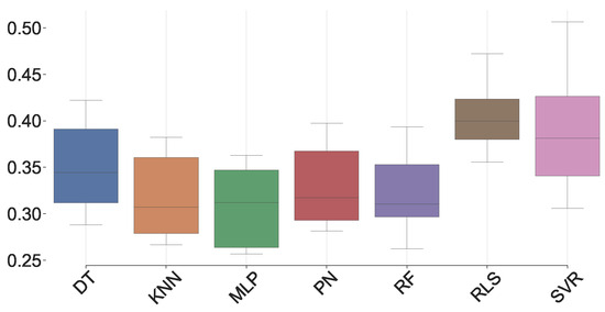
Figure 5.
MSE boxplot.
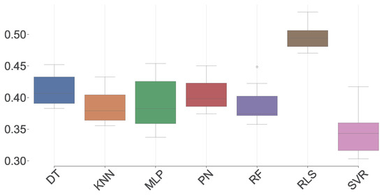
Figure 6.
MAE boxplot.
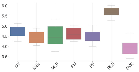
Figure 7.
SMAPE boxplot.
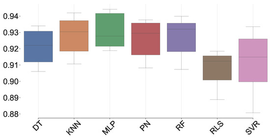
Figure 8.
boxplot.
At this point, the statistical analysis is made with these models and metrics. The metric was selected to determine whether there are significant differences between the results.
Firstly, the Kruskall–Wallis H-test was performed, obtaining a p-value of 0.0016. There are significant differences, as this value is lower than the value chosen of 0.05. To understand which differences are present, the Tukey test was carried out. This test takes the 21 possible different pairs and evaluates their differences, rejecting or accepting the hypothesis. The hypothesis was accepted in 17 pairs, meaning the models perform equally. The remaining five pairs present significant differences in terms of , as shown in Table 4.

Table 4.
Tukey test’s p-value in the rejected cases.
Table 5 corresponds with the metrics validation phase results. Values show a similar performance of every model with the training phase, indicating no overfitting. In this case, SVR and MLP are again achieving the best results, except for the MSE metric that is obtained by the polynomial regression, with a value of 0.3161 °C2.

Table 5.
Mean metric values in the validation phase of every model. The best results for each metric are highlighted in bold.
Figure 9 illustrates the values predicted by the MLP model during the validation phase. These predicted values are plotted against the actual values, demonstrating accurate forecasting, with all predictions closely aligning with the optimal diagonal dotted line. It is highlighted that there is no very high residual error, the most significant error being less than 2.7 °C.
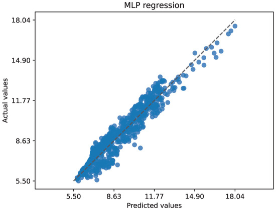
Figure 9.
MLP prediction vs actual plot in the validation phase.
5. Conclusions and Future Work
In this paper, a machine learning-based approach has been proposed to predict the output temperature of a horizontal geothermal heat exchanger of a bioclimatic house. Considering that multiple sensors are installed under the ground, this methodology aims to reduce installation and maintenance costs by minimizing the number of sensors used to perform the prediction. In this sense, the models could also be used to predict obstructions inside the exchanger.
Other advantages of applying this methodology include detecting possible physical sensor reading deviations. Furthermore, it can be used to predict the behavior of the heat exchanger to give information to the overall energy management system of the bioclimatic house. Moreover, the intelligent techniques proposed in this study could be deployed in an edge computing context, thus optimizing energy resources.
The methodology proposed in this study can apply to other cases, employing a significant dataset that represents the behavior of a different system or heat exchanger. Hence, this approach could be used to assess the feasibility of future installations. Nevertheless, the present research is focused on a unique installation. Thus, the modeling was carried out for the exchanger installed in this specific bioclimatic house. In this sense, the model validation and test stages have been conducted using the available dataset.
Several ML regression techniques were applied, and promising results were achieved. Specifically, the MLP technique obtains a good prediction, committing only a mean absolute error of 0.4204 °C and a mean squared error of 0.3887 °C2 while obtaining a symmetric mean absolute percentage error of 4.6589%. The coefficient of determination also obtains a high value of 0.9308, indicating that the regression line fits well with the ground values.
Assessing the performance of a geothermal heat exchanger is essential for optimizing energy consumption. In this sense, several strategies can be developed to improve energy efficiency and foster the implementation of predictive maintenance strategies. In addition, future applications, such as proper temperature regulation or electrical smart grids, may align with this proposal. In addition, given the multi-energy design of the bioclimatic house, future work may focus on the overall management of the whole thermal energy system.
More specifically, other approaches could be evaluated for implementing virtual sensors, in line with cost and maintenance optimization, focusing on sensor malfunction detection. Furthermore, other statistical or deep learning techniques such as ARIMA, LSTM, or GRU could be proposed to perform temperature forecasting, extending the prediction horizon.
Author Contributions
Conceptualization, A.D.-L. and F.Z.-G.; methodology, A.D.-L. and P.A.-B.; software, A.D.-L. and M.R.; validation, P.A.-B. and H.Q.; formal analysis, H.Q.; investigation, J.L.C.-R. and M.R.; resources, A.D.-L.; data curation, M.R.; writing—original draft preparation, P.A.-B. and J.L.C.-R.; writing—review and editing, F.Z.-G. and H.Q.; supervision, J.L.C.-R.; project administration, F.Z.-G. All authors have read and agreed to the published version of the manuscript.
Funding
Antonio Díaz-Longueira’s research was supported by the Xunta de Galicia (Regional Government of Galicia) through grants to Ph.D. (http://gain.xunta.gal), under the “Axudas á etapa predoutoral” grant with reference: ED481A2023072. This work has been supported by Xunta de Galicia through Axencia Galega de Innovación (GAIN) by grant IN853C 2022/01, Centro Mixto de Investigación UDC-NAVANTIA “O estaleiro do futuro”, which is ongoing until the end of September 2025. The support was inherited from both the starting and consolidation stages of the same project throughout 2015–2018 and 2018–2021, respectively. This stage is also co-funded by ERDF funds from the EU in the framework of program FEDER Galicia 2021–2027. CITIC is funded by the Xunta de Galicia through the collaboration agreement between the Consellería de Cultura, Educación, Formación Profesional e Universidades and the Galician universities for the reinforcement of the research centres of the Galician University System (CIGUS). Xunta de Galicia. Grants for the consolidation and structuring of competitive research units, GPC (ED431B 2023/49). This research is co-financed by the Interreg Atlantic Area Programme through the European Regional Development Fund, EAPA_00192022 SAtComm project.
Data Availability Statement
The data presented in this study are available on request from the corresponding author. The data are not publicly available as they were provided by a private company.
Conflicts of Interest
The authors declare no conflicts of interest.
Abbreviations
The following abbreviations are used in this manuscript:
| ANN | Artificial Neural Network |
| ARIMA | AutorRegressive Integrated Moving Average |
| DHW | Domestic Hot Water |
| DT | Decision Tree |
| GRU | Gated Recurrent Units |
| HSD | Honestly Significant Difference |
| KNN | K-Nearest Neighbors |
| LSTM | Long Short-Term Memory |
| MAE | Mean Absolute Error |
| ML | Machine Learning |
| MLP | MultiLayer Perceptron |
| MSE | Mean Squared Error |
| RBF | Radial Basis Function |
| ReLU | Rectified Linear Unit |
| RF | Random Forest |
| RLS | Recursive Least Squares |
| R2 | Coefficient of Determination |
| SMAPE | Symmetric Mean Absolute Percentage Error |
| SVM | Support Vector Machine |
| SVR | Support Vector Regression |
References
- Costantini, V.; Morando, V.; Olk, C.; Tausch, L. Fuelling the Fire: Rethinking European Policy in Times of Energy and Climate Crises. Energies 2022, 15, 7781. [Google Scholar] [CrossRef]
- Lund, J.W.; Toth, A.N. Direct utilization of geothermal energy 2020 worldwide review. Geothermics 2021, 90, 101915. [Google Scholar] [CrossRef]
- Hemeida, M.G.; Hemeida, A.M.; Senjyu, T.; Osheba, D. Renewable energy resources technologies and life cycle assessment. Energies 2022, 15, 9417. [Google Scholar] [CrossRef]
- Dickson, M.H.; Fanelli, M. Geothermal Energy: Utilization and Technology; Routledge: London, UK, 2013. [Google Scholar]
- Ozgener, L.; Ozgener, O. Monitoring of energy exergy efficiencies and exergoeconomic parameters of geothermal district heating systems (GDHSs). Appl. Energy 2009, 86, 1704–1711. [Google Scholar] [CrossRef]
- Anderson, A.; Rezaie, B. Geothermal technology: Trends and potential role in a sustainable future. Appl. Energy 2019, 248, 18–34. [Google Scholar] [CrossRef]
- Shortall, R.; Davidsdottir, B.; Axelsson, G. Geothermal energy for sustainable development: A review of sustainability impacts and assessment frameworks. Renew. Sustain. Energy Rev. 2015, 44, 391–406. [Google Scholar] [CrossRef]
- Omer, A.M. Ground-source heat pumps systems and applications. Renew. Sustain. Energy Rev. 2008, 12, 344–371. [Google Scholar] [CrossRef]
- Jenssen, T. Glances at Renewable and Sustainable Energy; Springer: Berlin/Heidelberg, Germany, 2013. [Google Scholar]
- Hou, G.; Taherian, H.; Song, Y.; Jiang, W.; Chen, D. A systematic review on optimal analysis of horizontal heat exchangers in ground source heat pump systems. Renew. Sustain. Energy Rev. 2022, 154, 111830. [Google Scholar] [CrossRef]
- Florides, G.; Kalogirou, S. Ground heat exchangers—A review of systems, models and applications. Renew. Energy 2007, 32, 2461–2478. [Google Scholar] [CrossRef]
- Rezaei, A.; Kolahdouz, E.M.; Dargush, G.F.; Weber, A.S. Ground source heat pump pipe performance with tire derived aggregate. Int. J. Heat Mass Transf. 2012, 55, 2844–2853. [Google Scholar] [CrossRef]
- Ozgener, O.; Ozgener, L. Modeling of driveway as a solar collector for improving efficiency of solar assisted geothermal heat pump system: A case study. Renew. Sustain. Energy Rev. 2015, 46, 210–217. [Google Scholar] [CrossRef]
- Ozgener, O.; Ozgener, L.; Goswami, D.Y. Experimental prediction of total thermal resistance of a closed loop EAHE for greenhouse cooling system. Int. Commun. Heat Mass Transf. 2011, 38, 711–716. [Google Scholar] [CrossRef]
- Aláiz-Moretón, H.; Castejón-Limas, M.; Casteleiro-Roca, J.L.; Jove, E.; Fernández Robles, L.; Calvo-Rolle, J.L. A fault detection system for a geothermal heat exchanger sensor based on intelligent techniques. Sensors 2019, 19, 2740. [Google Scholar] [CrossRef] [PubMed]
- Esen, H.; Inalli, M.; Sengur, A.; Esen, M. Performance prediction of a ground-coupled heat pump system using artificial neural networks. Expert Syst. Appl. 2008, 35, 1940–1948. [Google Scholar] [CrossRef]
- Yan, L.; Hu, P.; Li, C.; Yao, Y.; Xing, L.; Lei, F.; Zhu, N. The performance prediction of ground source heat pump system based on monitoring data and data mining technology. Energy Build. 2016, 127, 1085–1095. [Google Scholar] [CrossRef]
- Lu, S.; Li, Q.; Bai, L.; Wang, R. Performance predictions of ground source heat pump system based on random forest and back propagation neural network models. Energy Convers. Manag. 2019, 197, 111864. [Google Scholar] [CrossRef]
- Shin, J.H.; Cho, Y.H. Machine-learning-based coefficient of performance prediction model for heat pump systems. Appl. Sci. 2021, 12, 362. [Google Scholar] [CrossRef]
- Xu, X.; Liu, J.; Wang, Y.; Xu, J.; Bao, J. Performance evaluation of ground source heat pump using linear and nonlinear regressions and artificial neural networks. Appl. Therm. Eng. 2020, 180, 115914. [Google Scholar] [CrossRef]
- Baruque, B.; Porras, S.; Jove, E.; Calvo-Rolle, J.L. Geothermal heat exchanger energy prediction based on time series and monitoring sensors optimization. Energy 2019, 171, 49–60. [Google Scholar] [CrossRef]
- Ivanov, A.; Bezyayev, A.; Gazin, A. Simplification of Statistical Description of Quantum Entanglement of Multidimensional Biometric Data Using Symmetrization of Paired Correlation Matrices. J. Comput. Eng. Math. 2017, 4, 3–13. [Google Scholar] [CrossRef]
- Engel, Y.; Mannor, S.; Meir, R. The kernel recursive least-squares algorithm. IEEE Trans. Signal Process. 2004, 52, 2275–2285. [Google Scholar] [CrossRef]
- Weinberger, K.Q.; Saul, L.K. Distance metric learning for large margin nearest neighbor classification. J. Mach. Learn. Res. 2009, 10, 207–244. [Google Scholar]
- Imandoust, S.B.; Bolandraftar, M. Application of k-nearest neighbor (knn) approach for predicting economic events: Theoretical background. Int. J. Eng. Res. Appl. 2013, 3, 605–610. [Google Scholar]
- Czajkowski, M.; Kretowski, M. The role of decision tree representation in regression problems – An evolutionary perspective. Appl. Soft Comput. 2016, 48, 458–475. [Google Scholar] [CrossRef]
- Athey, S.; Tibshirani, J.; Wager, S. Generalized random forests. Ann. Stat. 2019, 47, 1148–1178. [Google Scholar] [CrossRef]
- Ostertagová, E. Modelling using polynomial regression. Procedia Eng. 2012, 48, 500–506. [Google Scholar] [CrossRef]
- Awad, M.; Khanna, R.; Awad, M.; Khanna, R. Support vector regression. In Efficient Learning Machines: Theories, Concepts, and Applications for Engineers and System Designers; Apress: Berkeley, CA, USA, 2015; pp. 67–80. [Google Scholar]
- Popescu, M.C.; Balas, V.E.; Perescu-Popescu, L.; Mastorakis, N. Multilayer perceptron and neural networks. WSEAS Trans. Circuits Syst. 2009, 8, 579–588. [Google Scholar]
- Ostertagová, E.; Ostertag, O.; Kováč, J. Methodology and Application of the Kruskal-Wallis Test. Appl. Mech. Mater. 2014, 611, 115–120. [Google Scholar] [CrossRef]
- Abdi, H.; Williams, L.J. Tukey’s honestly significant difference (HSD) test. Encycl. Res. Des. 2010, 3, 1–5. [Google Scholar]
Disclaimer/Publisher’s Note: The statements, opinions and data contained in all publications are solely those of the individual author(s) and contributor(s) and not of MDPI and/or the editor(s). MDPI and/or the editor(s) disclaim responsibility for any injury to people or property resulting from any ideas, methods, instructions or products referred to in the content. |
© 2024 by the authors. Licensee MDPI, Basel, Switzerland. This article is an open access article distributed under the terms and conditions of the Creative Commons Attribution (CC BY) license (https://creativecommons.org/licenses/by/4.0/).