Research on the Improvement of Cable Ampacity in Dense Cable Trench

Abstract

Due to the influence of many factors, distribution cables are often densely placed at the bottom of the cable trench. As a result, it is easy for distribution cables to become the thermal bottleneck of the whole transmission line. To address this dilemma, this paper establishes a finite element simulation model of a cable trench to analyze the hot spots of cables with different arrangements in the cable trench. Then, the model’s accuracy is verified based on real temperature rise experiments. For an arrangement with overheating risk, the ampacity improvement method of filling the cable trench with high-thermal-conductivity material was proposed, and the ampacity improvement effect under different filling ratios was assessed. Finally, combined with the analysis of economic benefit and cost, the method of determining the optimal filling ratio was used, and the impact resistance of the cables under the impact of new energy load was analyzed. The results indicate that, for the case of the optimal filling ratio, the cables in the dense cable trench showed superior impact resistance. The investigations in this paper make significant contributions to the promotion of the maximum utilization of cables.

1. Introduction

In recent years, with the promotion of renewable energy and the increase in electric energy demand, the load volatility of urban transmission lines has been intensified, the average load has increased continuously, and the peak time has been continuously extended [1,2,3,4]. This has led to an urgent need to improve the ampacity of existing distribution cables. When the transmission line current exceeds the ampacity of the cable for a long time, the cable’s insulation temperature exceeds the endurance temperature and the service life decreases dramatically, thus greatly increasing the risk of breakdown [5,6]. Under actual operating conditions, limited land resources, cable bracket aging, and a large number of new cable circuits lead to the cables being densely placed at the bottom of the cable trench, resulting in the cables overheating. Considering the various laying environments of cable, the thermal bottleneck points are taken as the goal of increasing the ampacity.

Currently, there are two main approaches to improving cable ampacity. The first approach is to fully explore the ampacity of the cable under its current operating conditions. In [7], a correction algorithm for the thermal resistance of a lining layer considering the dynamic shape factor was proposed, and the improvement effect of ampacity was verified by an experiment. In [8], an implement optimization method for a transient thermal model of cable insulation was proposed, and the effectiveness was verified by the finite element analysis method.

However, the improvement in ampacity achieved through this approach is limited. The second approach to enhancing cable ampacity is to improve the external heat dissipation environment of the cable. In [9], a study was conducted on the ampacity of submarine cables laid in rows, which was influenced by factors such as seawater velocity, seawater temperature, laying depth, and soil thermal conductivity. The effect of ampacity enhancement was verified by finite element simulation. Reference [10] calculated the conductor temperature for a typical water-cooled cable buried in a flat horizontal arrangement, and the simulation results showed that water-cooled pipes can effectively increase the ampacity. However, the thermal conductivity of water is not enough to meet the existing load demand, so existing studies have used different high-thermal-conductivity materials to reduce the thermal resistance of the external environment to improve the ampacity, and the improvement effect has been verified by experiments or finite element simulation [11,12,13,14,15,16,17,18,19]. In [20], an electromagnetic thermal coupling model of two parallel cables was established using the finite element method. The results showed that when the thermal conductivity of the backfill material was between 1.5 W/(m·K) and 2 W/(m·K), the cost performance was the best. Reference [21] analyzed the thermal conductivity characteristics of Lafarge Gruntar™ thermal backfill materials with different mass compositions. Thermal performance optimization procedures were then developed, and the heat dissipation characteristics were verified when backfill materials were added to the exterior of the cable ducts.

The above studies focus on the effect of using high-thermal-conductivity materials on the improvement of cable ampacity when the number of cables is small. However, in the case of dense cables in the distribution network, whether this scheme can still effectively increase the cable ampacity remains to be verified. In addition, because the renewable energy connected to the grid will cause strong fluctuations, whether the use of high-thermal-conductivity materials can provide the cable with sufficient impact resistance remains to be studied.

To address these issues, a simulation model for dense cable clusters was built to analyze the temperature distribution characteristics of different arrangements. The accuracy of the simulation model was verified by the high current temperature rise experiment. For the arrangement with the risk of overheating, using a high-thermal-conductivity material was proposed to increase the ampacity. Based on the simulation model, the enhancement effects of different filling ratios were studied. In order to save resources, a method for determining the filling proportion of high-thermal-conductivity materials was proposed, which considered the economic benefit and cost comprehensively. Finally, the load factor was put forward to change the fluctuating load into a steady load, and the simulation model was used to verify the impact resistance of the cable. This paper verifies the effect of high-thermal-conductivity material to improve the ampacity and impact resistance of dense cable clusters. It provides a technical guidance for maximizing the utilization of cable resources and renewable energy into the grid.

2. Analysis of Overheating Causes of Dense Cable Trench by Simulation

In actual operation, the arrangement of cables in the cable trench may deviate from the ideal arrangement specified in the engineering design standards. This can be due to factors such as the construction mode of the cables and the need for power outage maintenance. Additionally, the increasing load on the system may lead to a situation where the number of transmission circuits exceeds the number of designed cable supports. As a result, new cables are often placed at the bottom of the cable trench in a one-line arrangement. To explore the influence of two arrangements on the temperature distribution of the cable group, a finite element simulation model is designed to obtain the temperature distribution cloud map.

Based on the actual structural parameters of the 20 kV 3 × 35 mm² distribution cable, this paper builds finite element simulation models for both the ideal arrangement and the one-line arrangement.

Table 1. Structure and material parameters of 20 kV 3 × 35 mm² XLPE cable.

Structure	Material	Inside Diameter (mm)	External Diameter (mm)	Thermal Resistivity (K·m/W)	Heat Capacity (J/(m3·K))
Conductor	Copper	0	7	2.5 × 10−3	4.34 × 106
Conductor shield	Polyolefin	7	8.6	2.63	2.16 × 106
Lagging	Crosslinked polyethylene	8.6	19.6	3.5	3.03 × 106
Isolated shield	Polyolefin	19.6	21.2	2.63	2.16 × 106
Metal shield	Copper	21.2	21.5	2.5 × 10−3	4.34 × 106
Filler layer	Polypropylene fiber	21.5	48.0	5.24	1.73 × 106
Inner sheath	PVC	48.0	51.0	7.14	1.46 × 106
Shield	Steel	51.0	52.0	2.2 × 10−2	3.53 × 106
Outer sheath	PVC	52.0	57.4	7.14	1.46 × 106

provides the internal dimensions and physical parameters of the cable. To improve computational efficiency, this paper classifies the conductor shield and insulation shield as part of the insulation layer, considering their relatively small thickness [2]. Additionally, this paper neglects the influence of the steel frame in the model establishment due to its high thermal conductivity and small contact area with cables.

The boundary conditions of the heat transfer problem can be divided into three categories: the first is the known boundary temperature, and the boundary equation is shown in Equation (1):

$$\left\{\begin{array}{c}{\left.T\right|}_{\Gamma }=T_w\\ {\left.T\right|}_{\Gamma }=f(x,y,t)\end{array}\right.$$

(1)

where Г is the boundary of the object, T_w is a known boundary temperature (°C), and f(x,y,t) is the temperature function.

In the second category, the normal heat flux is known, and the boundary equation is shown in Equation (2):

$$\left\{\begin{array}{c}{\left.\lambda \frac{\partial T}{\partial n}\right|}_{\Gamma }+q_w=0\\ {\left.\lambda \frac{\partial T}{\partial n}\right|}_{\Gamma }+g(x,y,t)=0\end{array}\right.$$

(2)

where q_w is the known heat flux and g(x,y,t) is the heat flux function.

The third category is the convective boundary condition, and the boundary equation is shown in Equation (3):

$${\left.-\lambda \frac{\partial T}{\partial n}\right|}_{\Gamma }={\left.h(T-T_f)\right|}_{\Gamma }$$

(3)

where h is the convective heat transfer coefficient of the object surface and T_f is the temperature of the surrounding fluid.

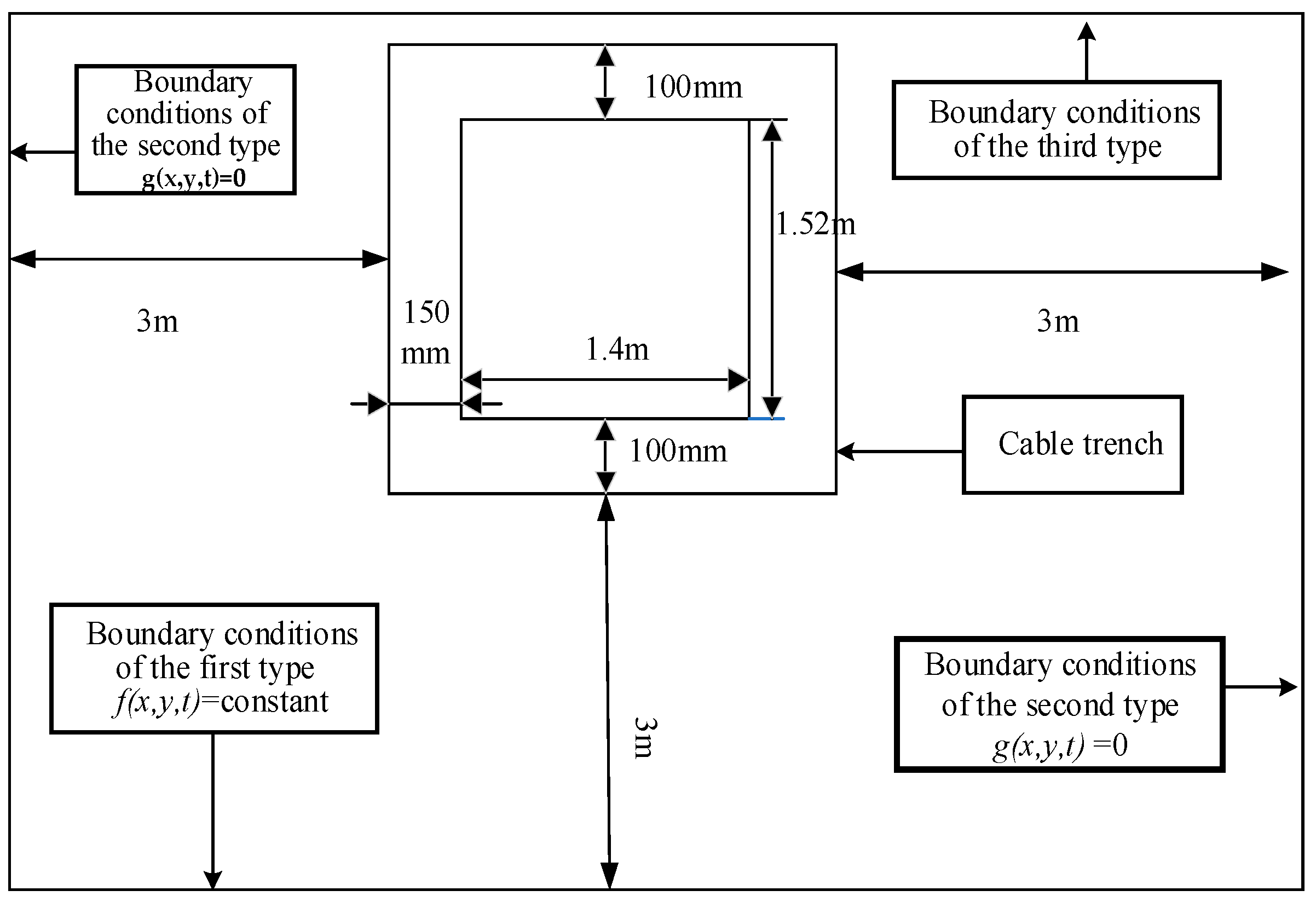
When cables are laid in cable trenches, their heat dissipation is influenced within a certain range. It is generally recognized that the soil temperature undergoes more significant changes within a 2 m distance from the cables, while farther away from the cables, the soil temperature tends to stabilize. Therefore, to improve the calculation accuracy, the left and right boundaries, as well as the lower boundary, were set at a distance of 3 m from the outer wall of the cable trench. The soil on the lower boundary could then be set based on the first type of boundary condition, which is a known boundary temperature. The soil on the left and right boundaries of the cable trench, being far away from the heat source, could be assumed to have an almost zero normal heat flux. This corresponds to the second type of boundary condition. The surface soil and the outer wall of the cable trench were in contact with the ambient air, which had a large enough domain that its temperature was not influenced by the heat dissipation from the cables. Hence, the boundary conditions at these locations can be considered as the third type of boundary condition. According to the heat transfer characteristics of cables laid in a cable trench, the boundary conditions around the cable trench were set as shown in Figure 1.

For two-dimensional simulation models, free triangle mesh, free quadrilateral mesh, and other meshes can be used for meshing. Since the free triangle mesh has the advantages of strong adaptability and fast delineation based on meeting the calculation accuracy, the free triangle mesh was used to mesh the model. The parameters of the surrounding medium material are shown in

Table 2. The parameters of the surrounding medium material.

Categories	Value
Cable surface heat radiation rate	0.95
Thermal emissivity of the inner wall of cable trench	0.85
Surface soil convective heat transfer coefficient	12.5 W/(m2·K)
Deep soil temperature	20 °C
Ambient temperature	30 °C

, and the thermal field parameters are shown in

Table 3. The thermal field parameters.

Categories	Concrete Walls	Air	Soil
Thermal conductivity(W/(m·K))	0.8	k(T)	1.2
Heat capacity at constant pressure (J/(kg·K))	1050	Cp(T)	1100
Density/(kg/m3)	1750	rho(pA,T)	2000
Ratio of specific heats	/	1.4	/
Dynamic viscosity (Pa·s)	/	eta(T)	/

.

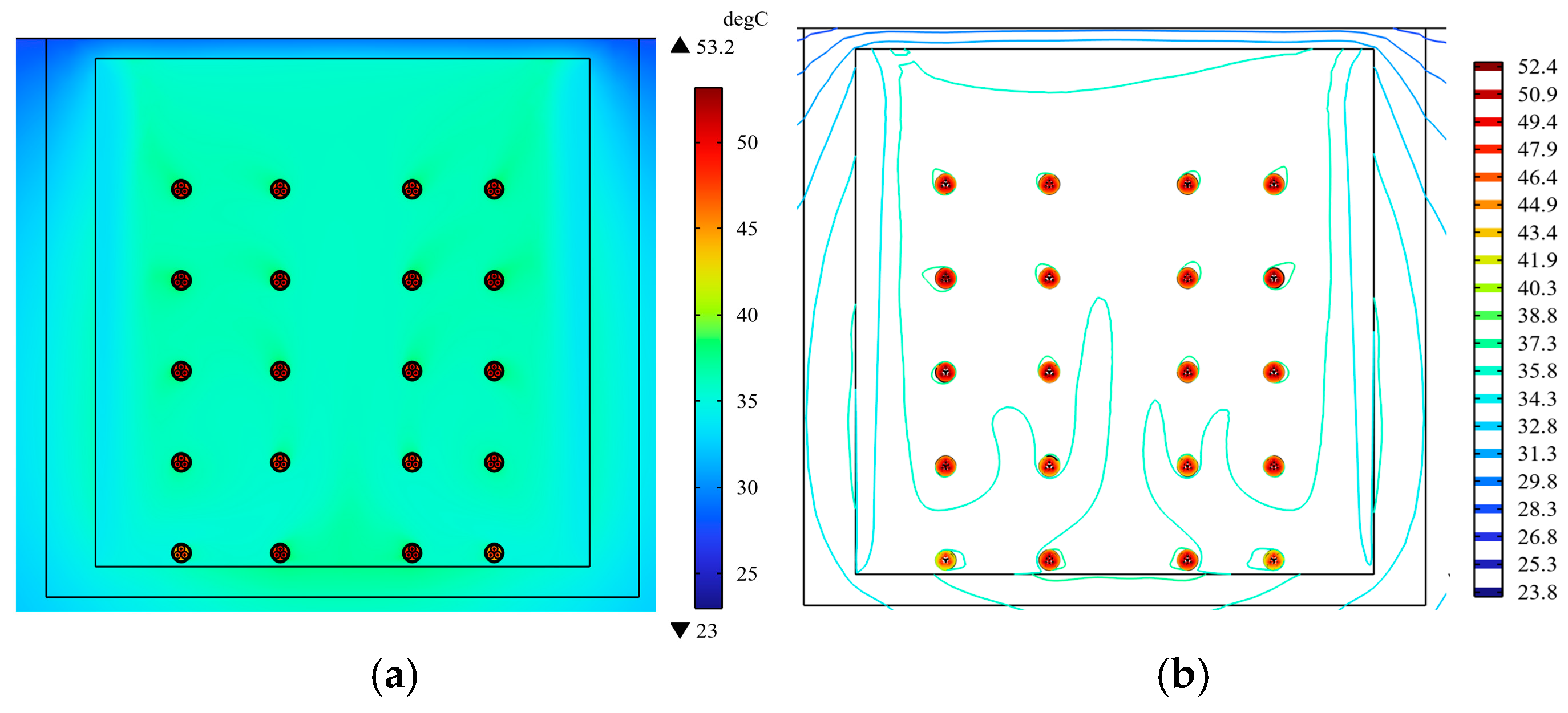
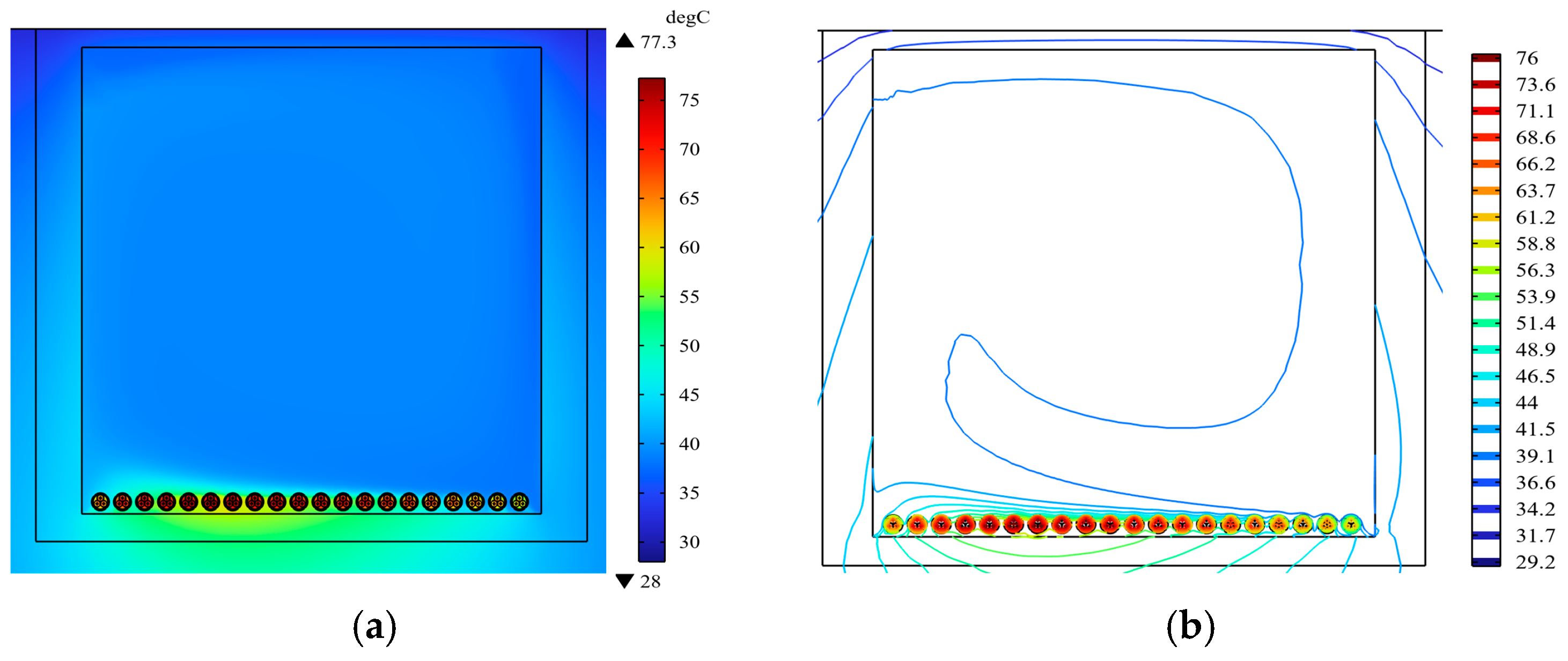
We set the load current of each cable in the model to 100 A. The cloud map of the steady-state temperature distribution of the two arrangements is shown in Figure 2 and Figure 3.

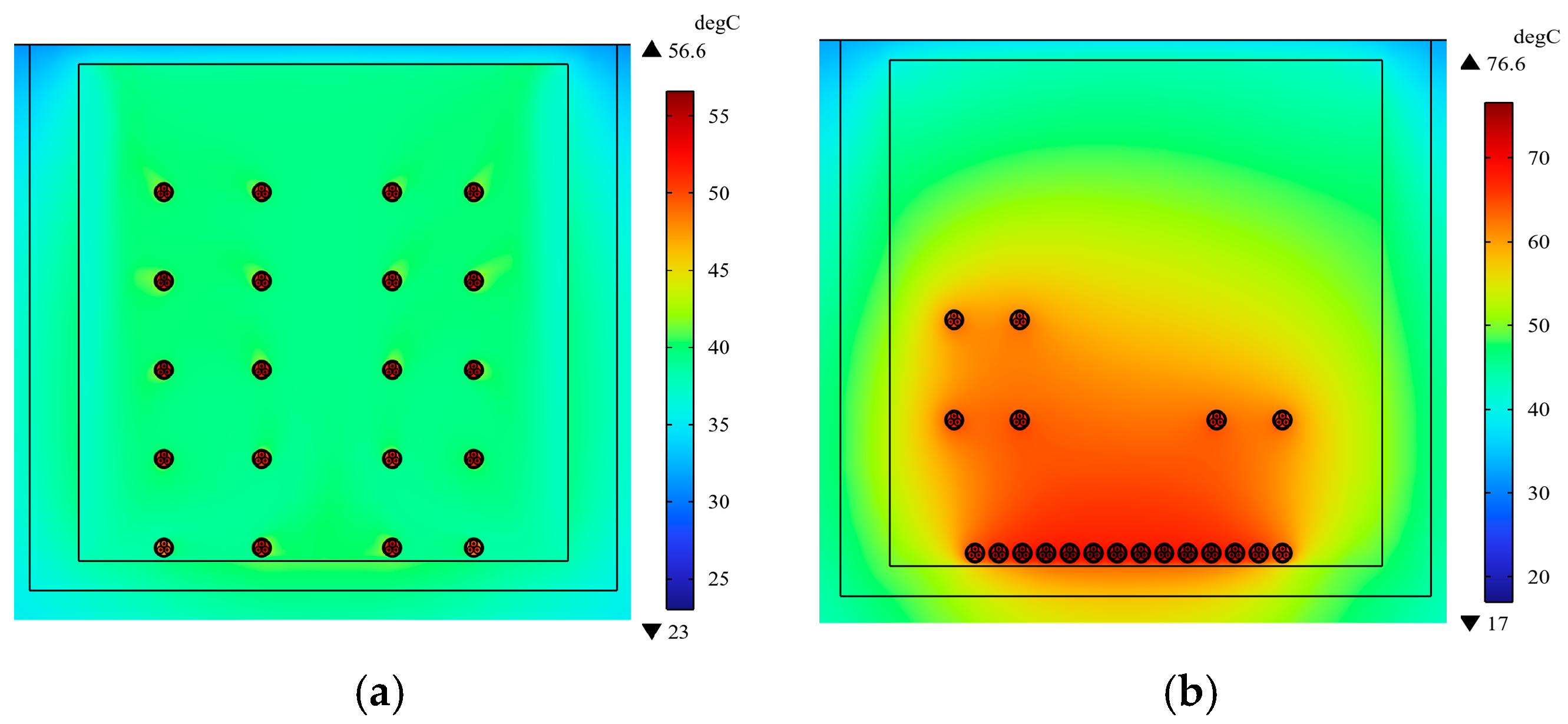
It can be seen from Figure 2 that when the ideal arrangement is adopted, the temperature distribution of the cable conductors in the cable trench is within the range of 50–53.2 °C. The second cable on the left side of the bottom has the highest temperature, 53.2 °C, and the second cable on the top left has a minimum temperature of 50 °C, with a difference of 3.2 °C. When the cables in the cable trench are arranged in this way, there is little difference in the cable’s temperature at different positions, and the ampacity seems balanced.

It can be observed from Figure 3 that when the one-line arrangement is utilized, the temperature of the conductor located in the middle reaches a maximum of 77.3 °C. On the other hand, the temperature of the conductors at both ends is at its minimum, measuring 60 °C. The temperature of the middle cable conductor is 17.3 °C higher than that of the conductors at the left and right ends. The temperatures of the cables at different positions in the cable trench are significantly different, and the transport potential is low.

According to the analysis of Figure 2 and Figure 3, it can be seen that the maximum difference in temperature shown in the conductor distribution cloud map between the ideal arrangement and the one-line arrangement is 24.1 °C, and the utilization of the ampacity of the one-line arrangement is not high. The main reason for this is that the spacing of the cable group in the ideal arrangement is 0.23 times larger than the cable diameter, and the mutual heat effect of the cables is very uniform, so the temperature distribution of the cable group is relatively uniform as well. The distance between the cables in the one-line arrangement is less than 0.23 times the cable diameter, resulting in heat dissipation difficulties, and the mutual heat effect of the cable groups is very uneven.

To investigate the impact of cable spacing on the temperature distribution, the cable spacing is varied, and the data for the maximum conductor temperature are obtained as shown in

Table 4. Maximum temperature of the cable conductor at different spacings.

Cable Spacing (m)	Maximum Temperature of Conductor (°C)	Minimum Temperature of Conductor in Two Sides (°C)
0.06	79.8	62
0.065	79.1	61.9
0.07	78.6	61
0.072	77.3	60.7
0.075	76.9	60

.

The simulation results show that the maximum temperature of the conductor decreased with the increase in cable spacing, and the minimum temperature of the conductor also decreased with the increase in cable spacing. This further proves that the length of the spacing becomes an important factor affecting the temperature of the cable group.

3. Verification of Simulation Model of Dense Cable Trench

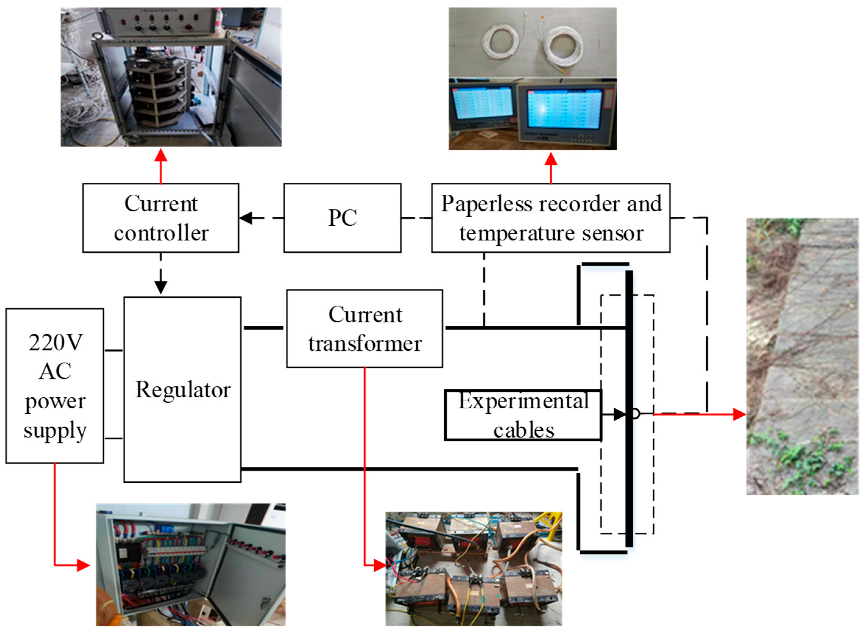
To validate the accuracy of the finite element simulation model for a dense cable trench, a cable temperature rise test was conducted on a multi-loop distribution cable. The cable model chosen for the experiment was YJV22-12/20 kV-3 × 35 mm². The cable temperature rise test platform consisted of two parts, as shown in Figure 4.

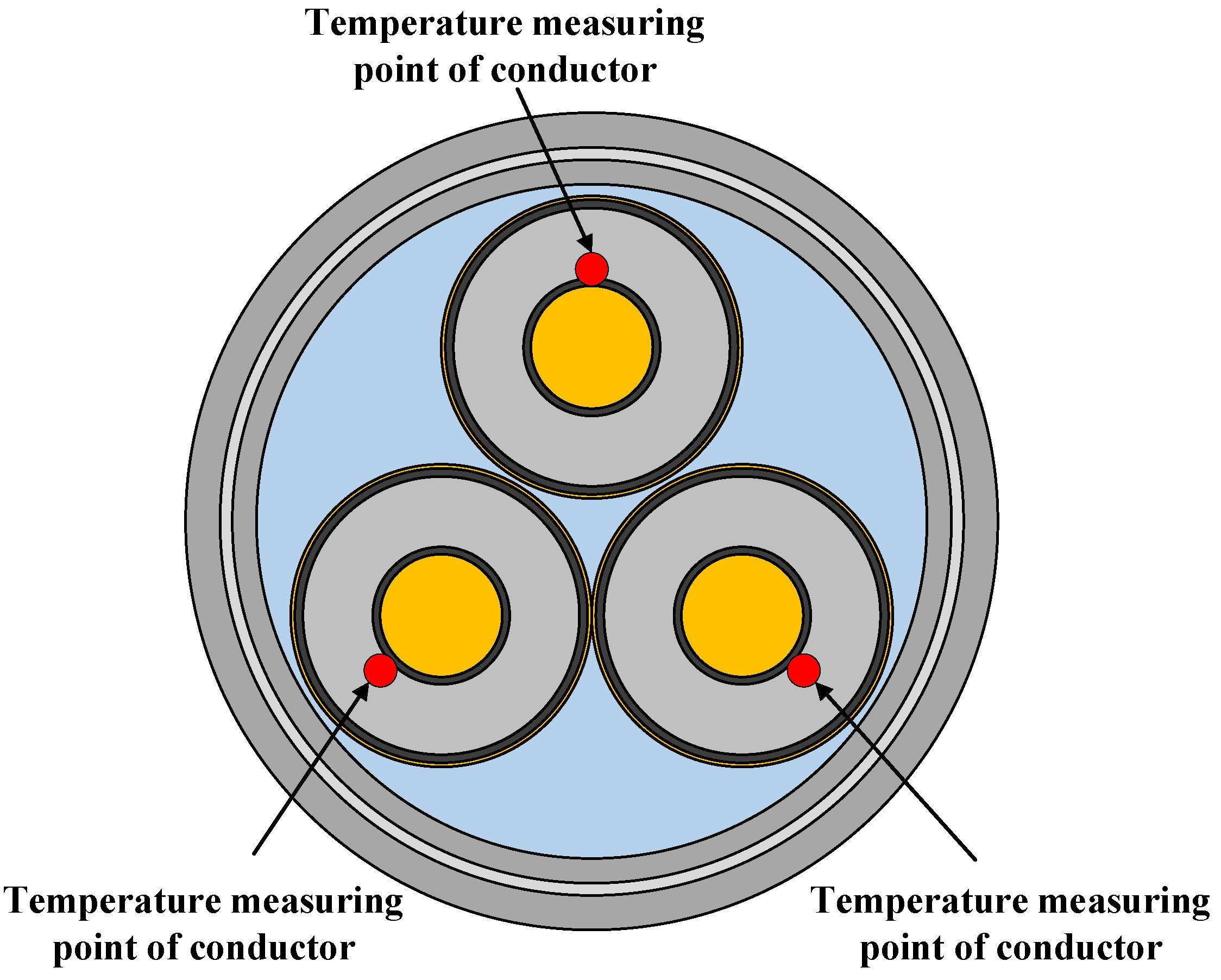
The first part was the high-current-generating system, which consisted of a 220 V AC power supply, a voltage regulator, a current transformer, a paperless recorder, a PC and, a PLC current controller. The high-current-generating system achieved automatic control of the test cable load according to the setting result of the PC. The second part was the temperature measurement system, which consisted of a temperature sensor (PT1000) and a paperless recorder. We arranged temperature sensors in the cable conductor and the external environment to achieve the collection of conductor temperature data and environmental temperature data. The test cable conductor temperature measurement point arrangement schematic diagram is shown in Figure 5.

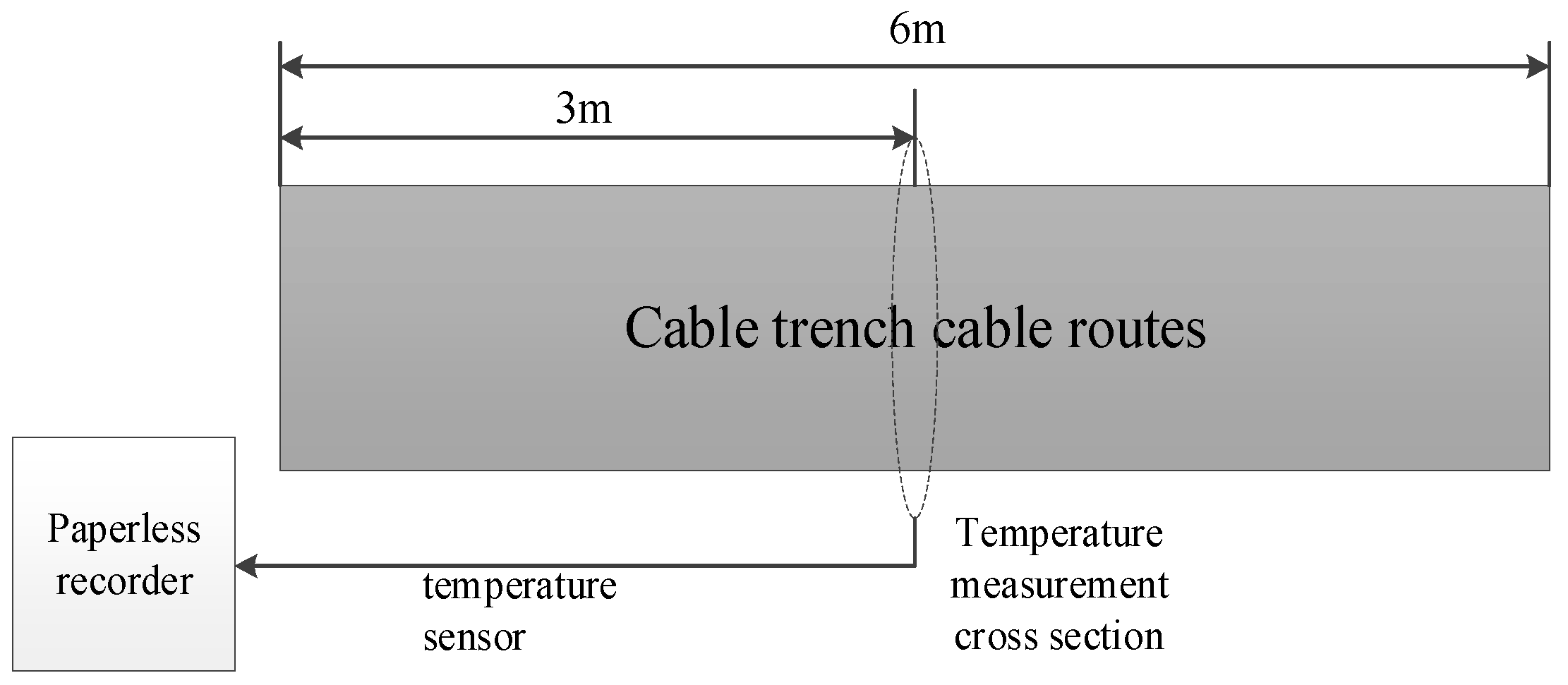
In order to reduce the impact of axial heat transfer on the measurement results, all temperature measurement positions were set in the cable midpoint within 0.1 m, as shown in Figure 6.

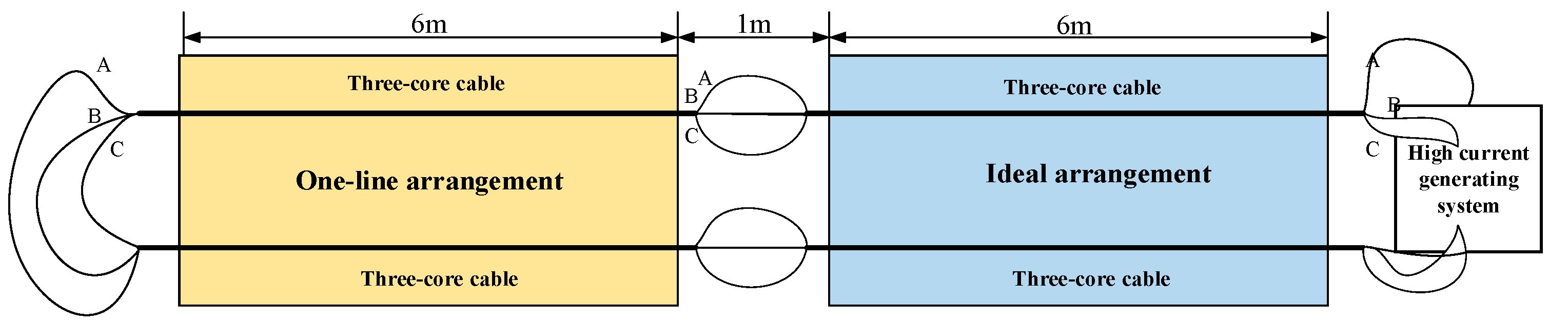
Temperature sensors transmitted the measured temperature data to the paperless recorder, which transmitted the collected temperature data to the terminal computer to realize a visual display of temperature data. The cable trench selected for the experiment, in which 20-circuit three-core cables were laid, was 1.52 m high and 1.4 m wide, and 12 m long. The ambient temperature was 30 °C, and the cable trench was divided into two sections: one was an ideal arrangement and the other was a one-line arrangement, as shown in Figure 7. To reduce the influence of cable axial heat transfer on the cable radial temperature distribution, the cable trenches of both laying methods were 6 m long. In addition, to ensure that the cable currents under the two laying methods were the same, the two sections of the cable were connected by wires in the middle.

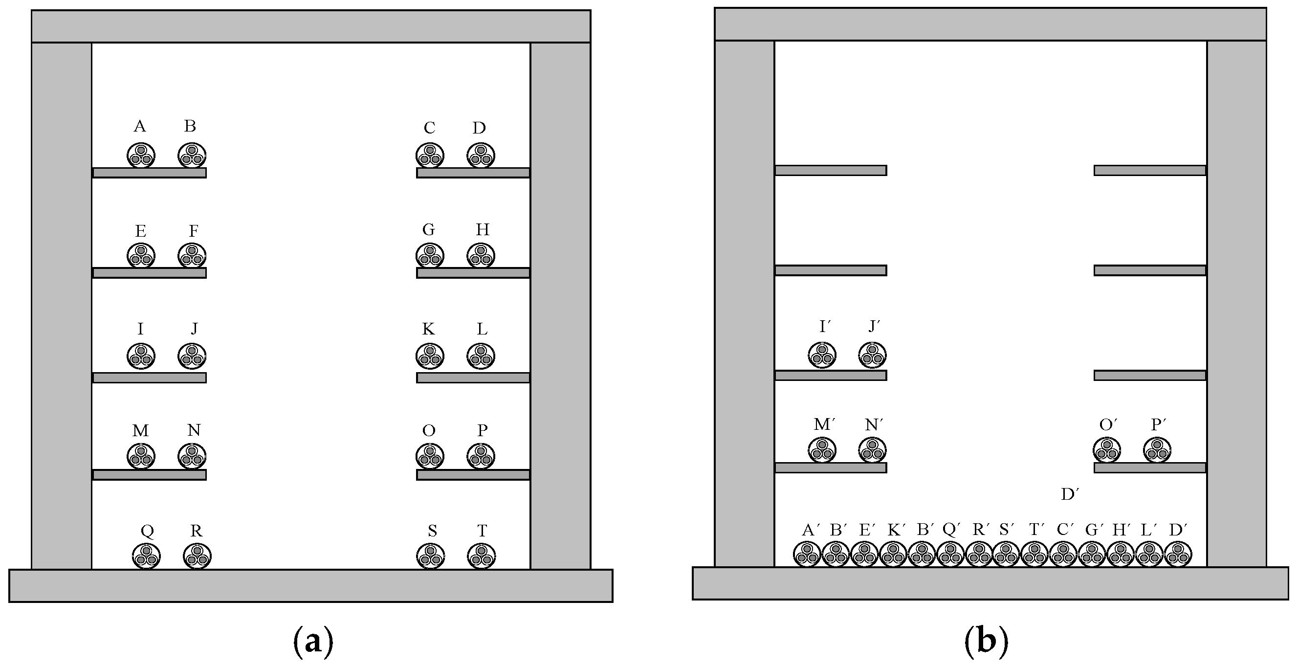
For the one-line arrangement, 16 one-line arrangement cables were placed at the bottom of the trench due to the limited space, and the other 4 were placed on the cable bracket. The three thermal resistors that measured the conductor temperature of the cable group were arranged 120° apart on the same diameter surface. Figure 8 shows the cable group arrangement. From left to right and from top to bottom, the cables that were ideally laid are numbered from A to T. The cables that touched each other are numbered from A’ to T’.

During the experiment, a current of 100 A was applied to the cable through the high-current-generating system, and a paperless recorder was used to record the average of the three conductor temperatures of the cables when the two arrangements reached a steady state. To ensure the results of RTD measurements for the results of full contact with the conductor, the conductor temperature measurement point took the highest temperature point.

According to the model established in Section 2, the temperature distribution cloud maps of the two arrangements were obtained in combination with the test conditions, as shown in Figure 9.

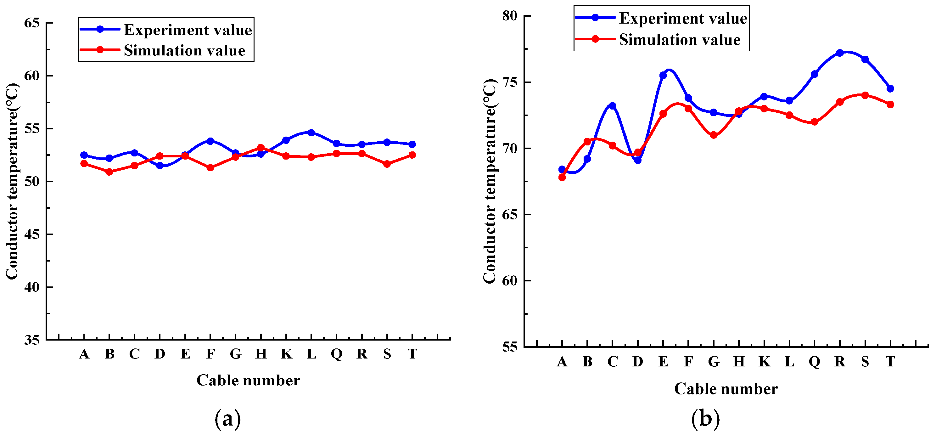
Combined with the above analysis, when the cable separation was greater than 0.23 times the cable diameter, the cable mutual heat effect had little influence on the temperature between cables, and the cable group temperature distribution was uniform. Therefore, this paper mainly analyzes the experimental temperature value of the one-line arrangement and the corresponding simulation value. Figure 10 shows the comparison between the measured cable temperature distribution and the simulated cable temperature distribution in the two modes.

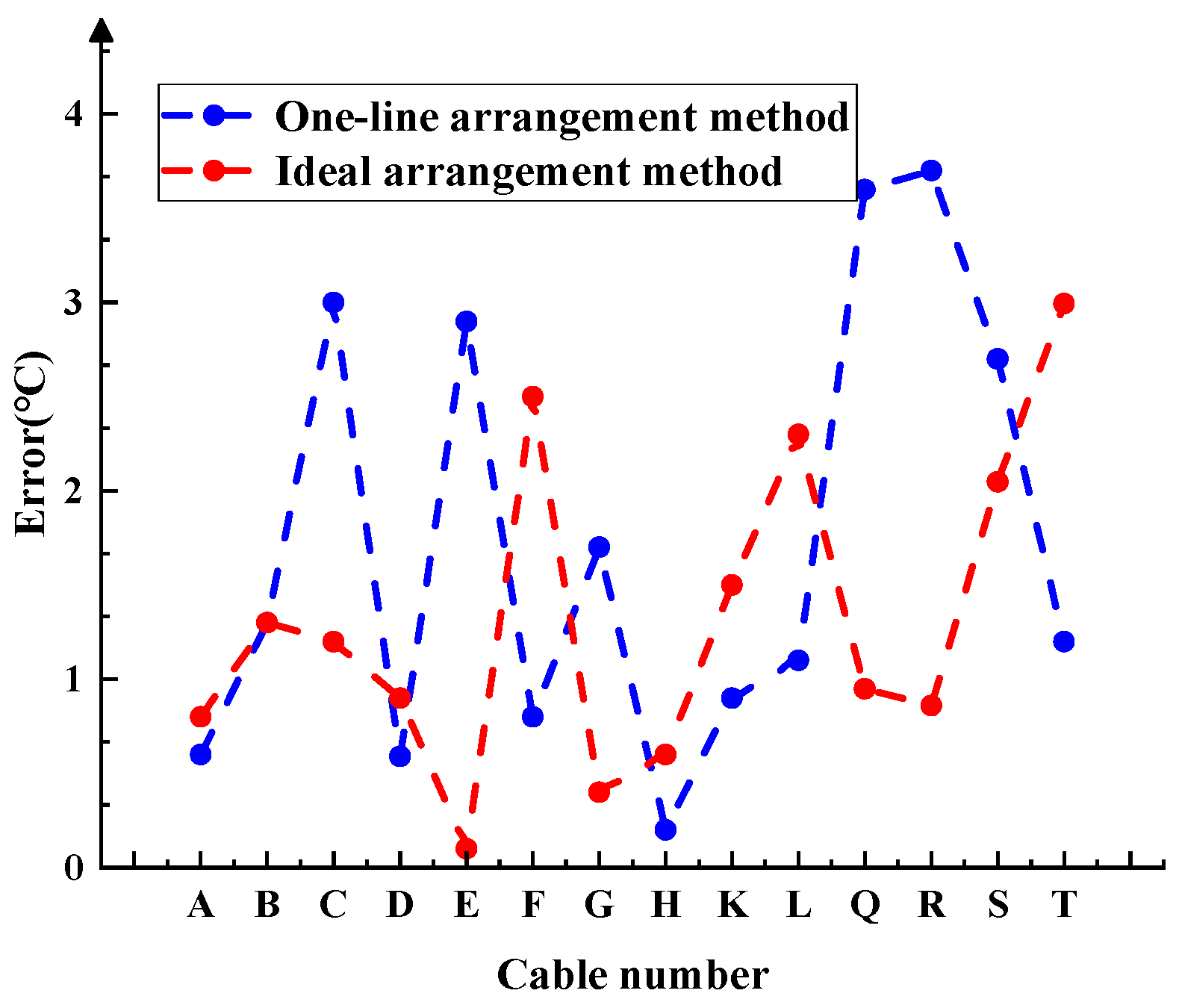
According to Figure 10, it can be seen that under the ideal arrangement, the temperature distribution in the cables was uniform, maintained between 50 and 53 °C. In the case of the one-line arrangement, the highest temperature of the cable reached 77.2 °C, the lowest temperature of the cable on the edge side was 68.4 °C, and no temperatures exceeded 70 °C. The temperature of the one-line arrangement was about 20 °C higher than the ideal arrangement. The correctness of the temperature distribution difference analysis of the above simulation model is demonstrated by the experimental data. To verify the correctness of the simulation model more intuitively, the error analysis was drawn by subtracting the experimental value from the simulation value, as shown in Figure 11.

Figure 11 shows that the maximum temperature error between the experimental value and the simulation value of the cables in one-line arrangement was 3.7 °C, and the maximum error between the experimental value and the simulation value in the ideal arrangement was 3 °C. Both errors were within the allowable range of experimental errors, which indicates that both the ideal arrangement and the one-line arrangement can reflect the temperature distribution of the cable group well.

4. Temperature Optimization Scheme of Dense Cable Trench

The experiments and simulation analysis above suggest that the mutual heat effect of the ideal arrangement was very balanced, and the conductor temperature was lower with the same load. However, the unbalanced mutual heat effect of the one-line arrangement led to the cables overheating. Moreover, due to the influences of various factors, the one-line arrangement has become a commonly used arrangement in actual operation. Therefore, for the one-line arrangement, this paper puts forward the use of high-thermal-conductivity material to reduce both the external thermal resistance and the influence of mutual heat.

In this paper, the ability of high-thermal-conductivity material to increase ampacity was investigated first. The modeling of the finite element simulation model was the same as that in Section 2. The air in the trench was replaced by the high-thermal-conductivity material, and the external ambient temperature was set at 30 °C. The thermal conductivity of the high-thermal-conductivity material was 3 W/(K·m), and the settings of other parameters were consistent with the above finite element simulation. 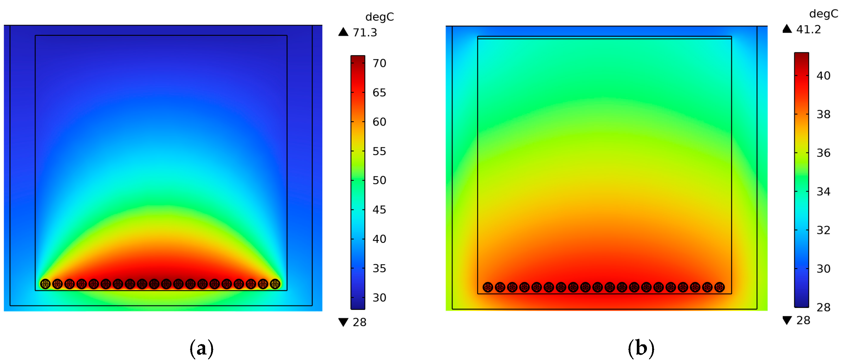Figure 12 shows the conductor temperature distribution when the high-thermal-conductivity material was not filled, and the filling rate was 100%. The results show that when other settings were all the same, the maximum temperature of the one-line arrangement with 100% filling rate was 41.2 °C, 30.1 °C lower than that without filling, and the improvement effect was drastically obvious.

From the analysis above, it can be seen that there was an air domain with poor circulation in the cable trench, which led to an overheating phenomenon in the cable trench. The high-thermal-conductivity material was able to effectively reduce the equivalent thermal resistance of heat transfer between the cable surface and the surroundings, and then reduce the temperature of the cable surface.

To further study the improvement effect of ampacity when the high-thermal-conductivity material was filled with different proportions, the filling ratio was set from 0 to 1, and the step was 0.1 in this section. Table 4 presents the temperature differences between the highest temperature conductor and the lowest conductor, considering the same filling ratio. Additionally, it also shows the temperature difference between the highest conductor temperature after filling and the temperature without filling.

From

Table 5. Conductor temperatures at different filling ratios.

Filling Ratio	Maximum Temperature of Conductor (°C)	Maximum Temperature Difference	Cooling Range (°C)
0	71.311	12.8	0
0.1	51.757	5.7	19.554
0.2	48.97	4	22.341
0.3	47.307	4	24.004
0.4	46.086	2.6	25.225
0.5	45.236	2.3	26.075
0.6	44.495	2.2	26.816
0.7	43.805	2	27.506
0.8	43.202	2	28.109
0.9	42.551	1.9	28.76
1	41.196	1.7	30.115

, it can be seen that when the filling ratio was 0.1, the maximum conductor temperature decreased by 19.5 °C compared to that without filling. This is because the thermal resistance between the cable and the bottom was greatly reduced due to the presence of the high-thermal-conductivity material, so the cable temperature was effectively reduced. However, with the increase in the filling ratio, the conductor temperature dropped slowly. When the filling ratio was 0.2, it only decreased by 2.8 °C based on the filling ratio of 0.1, because in this situation, it only increased the heat transfer area between the high-thermal-conductivity material and the trench wall, and the improvement in ampacity was not obvious. The maximum temperature difference of the conductor decreased with the increase in the filling ratio. The maximum temperature difference was 12.8 °C when the filling ratio was 0.1 and 5.7 °C when the filling ratio was 0.2. The maximum temperature difference tended to be stable as the filling ratio increased, and the maximum temperature difference was only 1.7 °C when the filling ratio was 1. This indicates that the high thermal conductivity of different filling ratios had an improvement effect, but the improvement effect did not increase with the increase in the filling proportion. Considering the filling cost of high thermal conductivity, it will be necessary to calculate the best filling proportion combined with economic benefits in a further study.

5. Method for Determining the Optimal Filling Ratio of High-Thermal-Conductivity Materials

The previous analysis highlights that there is a point of diminishing returns in terms of the gain in ampacity when the filling ratio reaches a certain value. Taking economic benefits into consideration, it becomes essential to develop a method for determining the optimal filling ratio of high-thermal-conductivity materials.

5.1. Cost Analysis

It is more practical to consider the construction, operation, and maintenance costs of high-thermal-conductivity materials over their entire service cycle. This approach allows for a comprehensive analysis of the economic feasibility, taking into account both the initial investment and the long-term costs associated with installation, operation, and maintenance. By considering the entire service cycle, a more accurate assessment of the economic benefits can be made. Therefore, the life cycle cost (LCC) calculation method was employed to determine the total cost of high-thermal-conductivity materials over their entire service cycle [22]. The LCC includes both the initial construction costs, encompassing material and labor expenses, and the ongoing monitoring, operation, and maintenance costs. This includes the cost of monitoring the performance of high-thermal-conductivity materials and the expenses associated with manpower and material resources required for activities such as water evaporation. By considering these factors, a comprehensive evaluation of the economic feasibility of high-thermal-conductivity materials can be conducted in a manner consistent with academic standards.

Based on the LCC method, the total life cycle cost of high-thermal-conductivity materials was calculated as follows:

Initial constructing costs of high thermal conductivity materials:

$$C_{c1}^{DP}=xy{h}_{1}az$$

(4)

where x is the length of the cable trench; y is the width of the cable trench; h₁ is the height of the cable trench; and a is the ratio between the height of the filling material and the height of the cable trench, called the filling ratio. z is the cost per unit volume of the high-thermal-conductivity material.

Monitoring, operation, and maintenance operating costs:

$$C_o^{DP}={\displaystyle \sum _{n=1}^L{C}_n^{DP}}{(1+i)}^{-n}$$

(5)

where $C_n^{DP}$ represents the operating costs incurred in year n, $C_n^{DP}$(1 + i)⁻ⁿ is the discounted present value of operating costs for n years, i is the discount rate, and L is the operating period.

5.2. Profits Analysis

The use of high-thermal-conductivity materials in cable filling significantly improves current-carrying ampacity and reduces power failure losses. As a result, the economic benefits primarily consist of increased revenue from electricity rates due to the improved ampacity and income generated by the reduction in power failure losses, which are calculated as follows:

Electricity revenue from filling high thermal conductivity materials K₁:

$$K_1=0.8UI\cdot 2\cdot 80\cdot L\cdot p_1$$

(6)

where L is the length of the operating period, U is the rated voltage, I is the increment of ampacity corresponding to the filling ratio a, and p₁ is the unit price per unit of electricity.

The power failure loss primarily refers to the economic loss experienced by power users during outages. The literature suggests that the cost associated with power outages per unit of power quantity A is dependent on the user composition type in the region and the proportion of ampacity λ_i (i = 1, 2,..., n) allocated to different users. The power outage cost per unit of electricity is A_i (i = 1, 2,..., n). A takes the weighted arithmetic average of A_i and is calculated as follows [23]:

$$A={\displaystyle \sum _{i=1}^n{\lambda }_i\cdot A_i}$$

(7)

Benefits for reducing power outage losses K₂:

$$K_2=0.8UI\cdot 2\cdot 80\cdot L\cdot A$$

(8)

where L is the operating period, U is the rated voltage, I is the increment of ampacity corresponding to the filling ratio a, and A is the stable value of power outage cost per unit of electricity.

5.3. Study Cases

To ensure the economic efficiency of transmission line operation, a calculation method for determining the optimal filling ratio of a general cable trench is proposed. In this method, the specific dimensions of the cable trench are considered. The cable trench is 5000 m long, 1.4 m wide, and 1.52 m high. The unit volume cost of filling this trench with high-thermal-conductivity material is given as 4000 RMB/m³. The cable model used was 20 kV-3 × 35 mm², and there were 10 circuits in total. The ampacity increment of the cable under different filling ratios was obtained through simulation.

Table 6. Key data of case analysis.

Parameter	Value	Unit
A	16.36	RMB
P1	0.5	RMB
L	10	RMB
i	6%	/
$C_{\mathrm{n}}^{DP}$	50,000	RMB

presents the key data of case analysis:

The profits of different filling ratios are calculated according to key data and cost and benefit calculation equations, as shown in

Table 7. Profits of different filling ratios.

Filling Ratios	Profits/RMB Ten Thousand
0.1	276.889
0.2	318.850
0.3	336.112
0.4	343.857
0.5	339.139
0.6	333.968
0.7	328.117
0.8	319.547
0.9	317.548
1	289.667

.

In Figure 13, the profit chart clearly demonstrates that the profit value increases as the filling proportion rises, specifically when it is less than or equal to 0.4. This trend culminates in the attainment of the maximum profit value, which amounts to RMB 3,438,557. However, it is observed that when the filling proportion exceeds 0.4, the profit begins to decrease as the filling proportion increases. Taking into account the economic benefits of power grid operation, it is recommended to maintain a filling ratio of 0.4 in this scenario. This choice ensures optimal profitability while considering the diminishing returns associated with higher filling proportions. The optimal filling ratios of cable trench models of other sizes can be analyzed by obtaining the key data of their operation. The optimal filling ratios for cable trench models of different sizes can be determined by analyzing key operational data.

6. Impact Resistance of Distribution Cable under Impact Load

Now, with our access to renewable energy sources and the popularity of electric vehicles, the load volatility of the distribution network has increased. The power consumption is higher at noon and in the evening. The added load of electric vehicles is a single-peak curve, and the peak position is close to that of the conventional load curve, but the duration of the peak of the added load is longer and lasts until midnight. Such load characteristics lengthen the second peak of the overall load curve, prolong the overall load fluctuation time, and then lead to the concentration of load over time. Due to the poor heat dissipation level of the surrounding environment where the cables are laid in the cable trench, overheating is prone to occur. Therefore, it is necessary to verify the impact resistance of the cable after filling the cable trench with high-thermal-conductivity material.

In this paper, the load factor is used to convert fluctuating load into constant load, and then we simulate different load fluctuation scenarios by changing the load factor to study the impact resistance. In the case that any load period of the load waveform can be known, the periodic waveform of the current heat loss can be obtained by dividing the load period into one hour. Then, the curve is expressed as a continuous step function change to obtain the average value, which is similar to the original value, and we use Y₀, Y₁, Y₂, ...Y₅ to represent this, thus calculating the periodic load current-carrying coefficient M [24].

$$M=\frac{1}{\sqrt{(1-K)\cdot Y_0+K\left\{B+\mu \times \left[1-\beta (6)\right]\right\}}}$$

(9)

$$\mu =\frac{1}{24}{\displaystyle \sum _{i=0}^{23}{Y}_i}$$

(10)

$$B=Y_0{\Phi }_0+Y_1{\Phi }_1+Y_2{\Phi }_2+Y_3{\Phi }_3+Y_4{\Phi }_4+Y_5{\Phi }_5$$

(11)

The parameters Φ₀~Φ₅ and [1 − β(6)] in the equation:

$$\left\{\begin{array}{l}{\Phi }_0=\beta \left(1\right)\\ {\Phi }_i=[\beta (i+1)-\beta (i\left)\right]\end{array}\right.$$

(12)

i takes the values of 1, 2, 3, 4, 5:

t = 3600i

(13)

$$k=\frac{W\cdot T_4}{\theta \left(\infty \right)}$$

(14)

where T₄ is the external thermal resistance, W is the total joule heat loss per cable at the rated current (W/m), and θ(∞) is the temperature rise of conductor above ambient temperature in steady state.

The method for calculating the M value is given above. When the load curve of the power grid is obtained, the value can be calculated by this method, and then the impact resistance of the cable under fluctuating load can be verified. Reference [24] studied the load characteristics of a city in the Pearl River Delta and obtained different values of the load factor M. In this paper, the larger value of 1.1–1.4 was selected to test the impact resistance of the cables under large load fluctuations. The simulation model for calculating the optimal filling ratio was used to obtain the maximum conductor temperature under different impact loads, and the result is shown in

Table 8. Maximum conductor temperatures under different impact loads.

Load Factor M	Conductor Temperature
1.0 times load	46.1
1.1 times load	49.7
1.2 times load	53.6
1.3 times load	57.8
1.4 times load	62.4

.

It can be seen from Table 8 that the maximum temperature of the conductor in the cable group also increased with the gradual increase in the overload multiple. The maximum temperature of the cables at 1.4 times the load was 62.4 °C, higher than that at 1.0 times the load, which was 16.3 °C. This shows that the high-thermal-conductivity material can effectively reduce the thermal resistance of the external heat transfer and effectively reduce the temperature of the entire cable group. Even with the maximum impact load, the highest conductor temperature of the cable group was far lower than the tolerance temperature of the crosslinked polyethylene, which had a large enough safety margin. Furthermore, the heat capacity of the high-thermal-conductivity material was 2500 J/(kg·K), which was much higher than the heat ampacity of the air of 1004 J/(kg·K), and the conductor temperature did not rise rapidly in the case of short-term large impact load. Due to the limited space, the transient characteristics after filling the high-conductivity material will be further studied. The steady-state and transient characteristics of the cable group after filling with a high-thermal-conductivity material show that the filling ratio not only met the requirements of economic benefit, but also provided the cables with excellent impact resistance.

7. Conclusions

In this paper, a simulation model of a cable trench was built, and its accuracy was verified through a temperature rise test. Then, the improvement effect of ampacity under different filling ratios was analyzed by the simulation, and the optimal proportion determination method was given in combination with economic benefits. Finally, the impact resistance of the cables was verified. The conclusions of this paper are as follows.

• The simulation results indicate that the conductor’s highest temperature is 53.2 °C when the ideal arrangement is used, while it reaches 77.3 °C in the one-line arrangement. The spacing between the cables significantly affects the temperature distribution characteristics. The experimental results for the latter arrangement, with a maximum error of 3.7 °C compared to the simulation results, validate the accuracy of the model.
• To solve the overheating problem of the dense cable group at the bottom of the trench, the ampacity-enhancing solution was proposed to reduce the external thermal resistance of the cable group by using a high-thermal-conductivity material. The simulation results show that when the filling ratio of high thermal conductivity material was 0.1, the cooling range reached 19.5 °C and the improvement in ampacity was significant, but tended to be stable with the increase in the filling ratio.
• Based on economic benefits, the optimal proportion of high-thermal-conductivity material filling was determined. The calculation results of the case showed that the economic benefit was the highest when the filling ratio was 0.4.
• The impact resistance simulation results demonstrated that the maximum temperature of the cable group when subjected to a load 1.4 times its normal ampacity reached only 62.4 °C. This temperature is significantly lower than the cable‘s maximum temperature rating of 90 °C, indicating excellent impact resistance.