Article

Design and Optimization of Cross-Corrugated Triangular Ducts with Trapezoidal Baffles Based on Response Surface Methodology and CFD

1
School of Mechanical and Electrical Engineering, Guilin University of Electronic Technology, Guilin 541004, China
2
Guangxi Special Equipment Inspection and Research Institute, Nanning 541004, China
3
College of Energy Engineering and Building Environment, Guilin University of Aerospace Technology, Guilin 541004, China
*
Authors to whom correspondence should be addressed.
Energies 2024, 17(10), 2335; https://doi.org/10.3390/en17102335
Submission received: 22 March 2024 / Revised: 29 April 2024 / Accepted: 9 May 2024 / Published: 12 May 2024

Abstract

:
Plate heat exchangers are widely used in the Heating, Ventilation, and Air Conditioning (HVAC) field. Cross-corrugated triangular ducts are commonly employed in plate heat exchangers. Inserting baffles into the cross-corrugated triangular ducts can improve the heat transfer performance of the plate heat exchangers. This study focuses on intricate interdependencies among the flow channel apex angle, the trapezoidal baffle inclination angle, baffle position, and Reynolds number (Re) on heat transfer and pressure drop using response surface methodology (RSM) and computational fluid dynamic (CFD). To identify the factors that maximize the Nusselt number (Nu) and minimize friction factor (f), the RSM is used to design factors, conduct numerical studies, and establish regression equations. The results show that the apex angle, baffle angle, X-direction position, and Re have significantly affected Nu and f. Compared to a non-baffled channel with the same apex angle and Re conditions, the optimized channel enhances heat transfer by 1.54 times and has an almost identical pressure drop. The inclined baffle significantly enhances comprehensive performance at low Re. The synergistic effect of the heat transfer and pressure drop is most optimal when the apex angle of the flow channel is 90°, the trapezoidal baffle inclination angle is 52.5°, and the Re is 1000, with the baffle position at 0.625H in the X-direction.

1. Introduction

Global climate change is one of the biggest challenges confronting the world. Reducing greenhouse gas emissions, especially carbon dioxide emissions, is critical for mitigating climate change. Therefore, countries around the world are taking active measures to promote carbon peaking and carbon neutrality. The building sector and building operations (including heating, cooling, lighting, and other electrical equipment) account for about 30% of global end-use energy consumption. In addition, the building sector and building operations account for 36% of energy-related carbon dioxide emissions [1]. The plate heat exchanger is a highly efficient and energy-saving piece of heat exchange equipment with proven heat transfer efficiencies of 1.2 to 2.1 times that of tube heat exchangers [2]. It is widely used in HVAC and other industrial fields, including electronic thermal management, aerospace, marine, and others [3,4,5]. Improvements in the energy efficiency of plate heat exchangers, even minor ones, can significantly impact building energy conservation and, by extension, global energy usage.
The plate heat exchanger utilizes adjacent corrugated plates stacked at an angle to a flow path, separating hot and cold fluids by directing them through different flow paths. The corrugated plates can be stacked in various ways, forming triangular, sinusoidal, square, trapezoidal, elliptical, and other shapes. Different corrugation profiles have a significant effect on heat transfer and flow characteristics [6]. Liao [7] compared the falling film flow characteristics of liquids on surfaces with three different corrugation shapes. He found that the triangular corrugated plate was more conducive to liquid film flow than sinusoidal and trapezoidal and the performance was most excellent at 75° over the range of triangular corrugation angles of 15°–75°. Younis [8] tested the effect of five different geometries, namely flat, sine, square, triangle, and sawtooth, on the heat transfer results and showed that the triangular corrugated channel allowed more heat transfer to the phase change material and accelerated the melting time of nanoparticles. Therefore, it is meaningful to have an in-depth investigation of the triangular flow channel. Figure 1 is a schematic of a cross-corrugated triangular heat exchanger. In Figure 1, the cold fluids flow directly in the Y axial direction, while the hot fluids flow directly in the Z axial direction. Therefore, the heat exchanger is a cross-flow heat exchanger. The cold and hot fluids in the exchanger exchange heat through the corrugated plates. Verdério Júnior [9] investigates the physical parameters of a flat plate with square, trapezoidal, and triangular corrugations and derives empirical formulas related to Nu and convective heat transfer coefficients. He also points out that the heat transfer area has a more significant effect on the heat transfer efficiency than the corrugation spacing. Easwaran [10] conducted a study on the corrugation angle β, corrugation depth-to-pitch ratio, and flat plate geometry of cross-corrugated triangular ducts. The study showed that Nu and f reached their maximum values when the corrugation angle is at 25° < β < 75° and that the corrugation depth to pitch ratio is positively correlated with them. Additionally, the plate length was found to be independent of the factors. Sarraf et al. [11] demonstrated, through computational fluid dynamics (CFD) analysis, that the Re or mass flow rate has an impact on the transition between two flow structures: ‘spiral flow’ and ‘cross flow’.
The shell and tube heat exchanger commonly employs the method of placing baffles to enhance fluid mixing and disturbance. This forces the fluid to pass through the tube multiple times, increasing turbulence and improving heat transfer. Cao [12] inserted helical baffles into shell and tube heat exchangers that significantly improved shell-side heat transfer and comprehensive performance. Handoyo [13] added triangular obstacles inside the V-shaped corrugated channel and studied the effect of the pitch between these obstacles on the heat transfer and pressure drop of the air inside. The researcher discovered that the flow became more turbulent due to the high velocity between the obstacles and the absorber plate. Additionally, the optimal distance between the obstacles was found to be equal to their height. This increases the internal friction and collision of the fluid, resulting in increased energy consumption. Karabulut [14] investigated a flow channel with an apex angle of 60° and a triangular baffle height of 0.5H at placement angles of 30°, 45°, 60°, and 90° and Re ranging from 1000 to 6000. The results of the study showed that the Nu for the 60° corrugated duct was 8.2% higher than that for the 90° corrugated channel at Re = 4000. Furthermore, at Re = 1000, the pressure drop in the 60° was 39% lower than that in the 90° corrugated channel. Alnak [15] analyzed the heat transfer, pressure drop, and thermodynamic characteristics of corrugated ducts with square baffles under the same conditions. The results showed that the Nu for the corrugated ducts with a square baffle at a 90° angle is 52.8% higher than that of 60° for the Re = 6000. Also, for Re = 1000, the pressure drop value with a 60° baffle angle is 65.97% lower than that of the 90° in the triangular corrugated duct. Akcay [16,17] carried out a numerical investigation on the hydraulic and thermal performance of pulsating flow in a periodic corrugated channel with discrete V-type winglets. It was found that the winglet geometry and a certain degree of inclination have a significant effect on the flow and heat transfer and that the perforated winglets can further reduce the friction factor.
We have conducted a few in-depth studies on corrugated ducts and baffles. Liang et al. [18] used a particle swarm optimization algorithm to optimize cross-corrugated triangular ducts and ascertained that the apex angle, the channel height, and the heat exchanger height affect the system performance. Feng and Liang et al. [19] analyzed the effects of different types of trapezoidal baffles on flow velocity and temperature distribution at an apex angle of 60°. They concluded that the trapezoidal baffle with an upper bottom width of 3/4W and a lower bottom width of W has the best comprehensive overall heat transfer performance. Based on this study, Li [20] includes consideration of the apex angle. The flow field is further complicated by the variation in apex angle and trapezoidal baffle position. The flow channel has the highest f, Nu, and PEC values when the baffles are in the center of the upper half of the channel. For most conditions, the baffle increases the comprehensive performance but for an apex angle of 120, the baffle may have the opposite effect.
The central composite design is an integral facet of the response surface methodology. It establishes a functional relationship between one or more factors and the response variable. This relationship is represented graphically to identify optimal conditions in the experiment. This methodology is suitable for multifaceted experiments involving multiple factors and varying levels, particularly in scenarios involving continuous variables [21]. Sharma [22] applied the response surface method and artificial neural network to optimize the geometry of curved trapezoidal winglets, resulting in improving the heat transfer efficiency and minimizing the pressure loss of the fin-and-tube heat exchanger. Yu [23] used the response surface methodology to investigate the correlation between four critical parameters of a parallel flow shell and tube heat exchanger with baffle and sinusoidal corrugated fins, fin pitch, fin amplitude, fin width, and Re. This analysis revealed the intricate relationships that govern thermal performance. A similar approach was used by Kola [24] in a study of double-tube heat exchangers. The significance of linear and interaction terms related to twist ratio, twist direction, and bond geometry on the response variable was revealed using analysis of variance (ANOVA). The results show that these factors have a significant effect. Rezaei [25] performed modeling of three factors of a spiral-tube heat exchanger and confirmed that the highest heat transfer efficiency was obtained at an exhaust diameter of 4 cm and a water flow rate of 6 L/min with six fins.
Previous research has made valuable contributions to the optimization of baffles in cross-corrugated triangular ducts. However, within a triangular corrugated channel, vertically arranged trapezoidal baffles enhance the flow but generate large pressure drops simultaneously. Inspired by the earlier work, whether to give the trapezoidal baffles a certain angle to neutralize this situation was considered. In practical engineering scenarios, there are complex relationships between corrugated plate geometric parameters and baffle placement that affect heat transfer and hydraulic performance. As many studies have failed to address the intricate interdependencies, this paper provides a holistic approach that employs RSM and CFD to systematically investigate the five factors of apex angle, trapezoidal baffle angle, X-direction position, Y-direction position, and Re. This approach indicates the degree of influence of the five factors on heat transfer and flow and ascertains the operating conditions for optimum performance. The study provides a reference to optimize the design of heat exchangers with cross-corrugated triangular channels.

2. Response Surface Design

Response surface design is an advanced Design of Experiments (DOE) technique that has significant utility in generating insights and optimizing responses. It is particularly effective in scenarios where response surfaces exhibit curvature. This technique is widely used to optimize models once important factors have been identified. The central composite design is the prevailing response surface design experiment. It is noted for its ability to adequately accommodate fully quadratic models. This section covers the efficient estimation of both first- and second-order terms, as well as modeling response variables with nonlinear curvatures. The second-order model is expressed as follows [26]:
y = b 0 + i = 1 k b i x i + i = 1 k b i i x i 2 + b i j x i x j + σ i < j
where y is the response variable; b0 is a constant; b1, b2, …, bk are the coefficients; x1, x2, …, xk are the values of the terms, and σ is the error term.
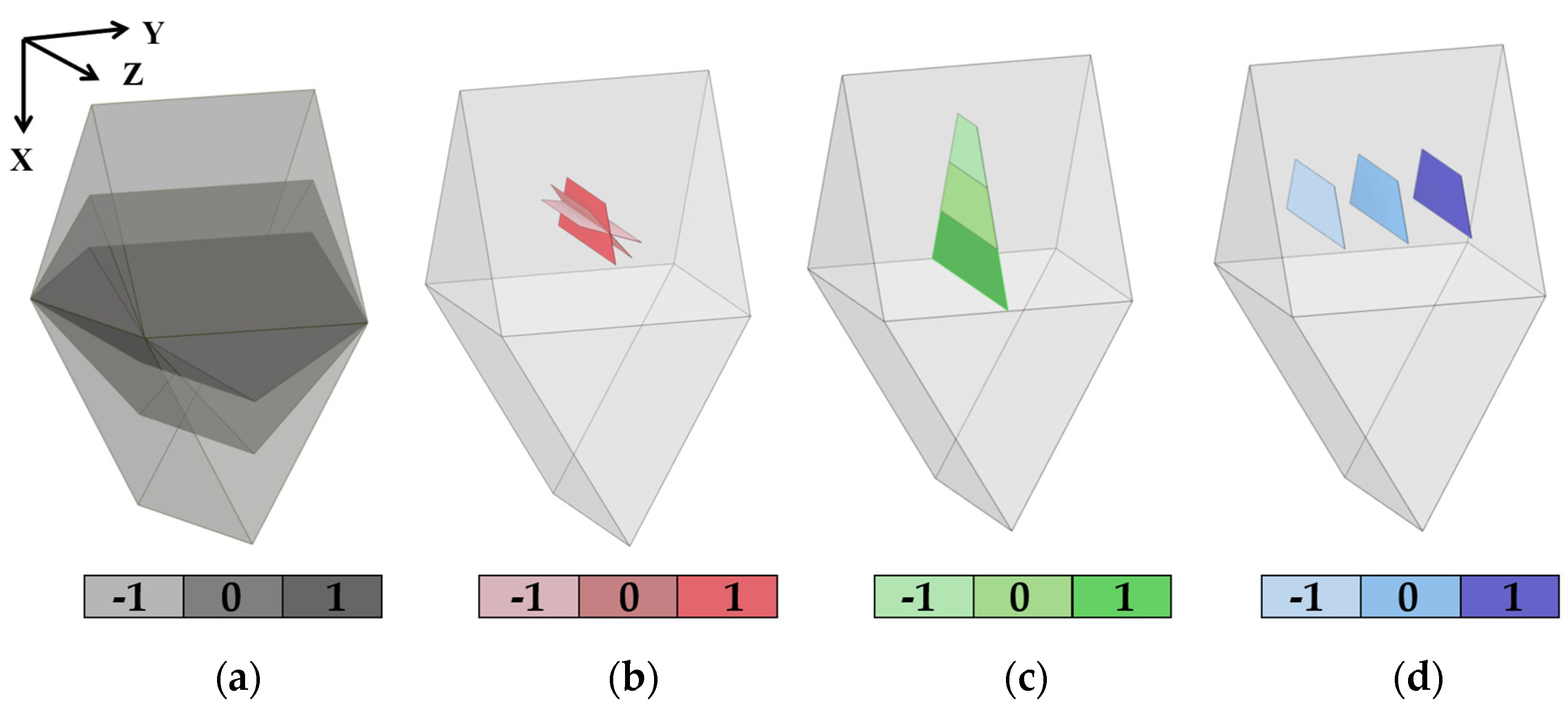
The study utilized Mintab v19 [26] software to perform a central composite design of cross-corrugated triangular flow channels with trapezoidal baffles. The parameters investigated included the apex angle of the flow channel, the trapezoidal baffle placement angle, the positions in the X and Y directions, and the Re. A compressive investigation was carried out using a five-factor two-level experimental design. The Nu and f were the response values targeted for optimization. Table 1 shows the high and low levels of each factor. For a better comprehension, Figure 2 illustrates the corresponding states within the unit flow channel.
In the factorial design, the factors and levels in Table 1 are utilized to create a design geometry matrix with N = 32, as shown in Table 2.
The numerical simulations were conducted based on the arrangement presented in Table 2 and the results are also listed in the table.

3. Model

3.1. Solution Procedure

The Reynolds number in this study ranges from 1000–3000. The working fluid is air, corresponding to a velocity of 1.12–5.85 m/s. This is the general working velocity in heat exchangers. Due to the periodic convergence–divergence characteristics of the fluid in the cross-triangular corrugated plate heat exchanger, the flow characteristics are complex and therefore simulated with a turbulence model [27]. The Reynolds Stress Model is the finest RANS turbulence model supported by Fluent, closing the equations by solving the Reynolds stress transport equation and the dissipation rate equation. It has the possibility of predicting complicated flows with higher accuracy and with high capability in modeling streamline curvature, vortex flow intensity, and strain rate [28,29]. Liu et al. [30] conducted a numerical simulation of the cross-corrugated triangular ducts using seven turbulence models. The results indicate that the Reynolds Stress Model provides more accurate predictions, with simulated values within 7% of the experimental values. Sharif et al. [31] used a Reynolds Stress Model to simulate unbaffled cross-corrugated triangular ducts with Re ranging from 310 to 2064, resulting in error within 5% of the experimental results. Therefore, the Reynolds Stress Model is adopted in this paper for the solution. For a detailed description of hydrodynamics governing equations, please refer to [28]. Below, we only present and explain the quantities relevant for the RSM analysis.
The hydraulic diameter of the channel can be defined by
D h = 4 V c y c A c y c
where Vcyc is the volume of a cycle, m3, and Acyc is the surface area of a cycle, m2.
The Reynolds number can be calculated by
R e = ρ u m D h μ
where um is the area-weighted average speed at the entrance, m/s.
The convective heat transfer coefficient is
h = c p ρ u m A c i ( T i T o ) A c y c Δ T m
where cp is the specific heat of the fluid, kJ/(kg·K); Aci is the cross-sectional area at the entrance or exit of a cell, m2; Ti and To are fluid temperatures at inlet and outlet, respectively, K; and ∆Tm is the logarithmic mean temperature difference between the wall and the fluid, which can be expressed as
Δ T m = ( T i T w ) ( T o T w ) l n T i T w T o T w
where Tw represents average surface temperature, K.
The Nusselt number is defined as
N u = h D h λ
where h is the convective heat transfer coefficient, W/(m2·K), and λ is the thermal conductivity of the air, W/(m·K).
The cell average friction coefficient can be expressed as
f = ( P i P o ) D h 1 2 ρ u m 2 L
where L is the length of a cell, m, and Pi and Po are the inlet and outlet pressures of a cell respectively, Pa.
Considering the comprehensive effects of the baffle on flow and heat transfer, the Performance Evaluation Criterion (PEC) was introduced as follows:
P E C = N u N u 0 ( f f 0 ) 1 3
where Nu0 is the value of Nu for unbaffled channels and f0 is the value of f for unbaffled channels.
Dimensionless temperature is defined as
T * = T T T w T
In the calculation, the governing equation is solved numerically using the finite volume method with Ansys Fluent v2021R2 [32]. A pressure-based solver with a pressure correction algorithm is applied. The diffusion term is discretized using a central difference scheme and the convection term is computed with second-order upwind accuracy. The solution algorithm is coupled. The convergence criterion is set to 10−4 for the continuity and momentum equations and for the energy equation it is set to 10−7.

3.2. Computational Domain

The study examines 10 triangular cells, with an illustrative example of a flow channel with an apex angle of 60° shown in Figure 3. Each cell has uniform dimensions: a length (L) and width (W) of 0.015 m and a corrugation height (H) of 0.01299 m. Although the length and width remain constant across the flow channel cells with different apex angles, the corrugation height varies with the apex angle. The corrugation heights for apex angles of 90° and 120° are 0.01066 and 0.00433 m, respectively. The figure shows a trapezoidal baffle with a 90° angle at 0.625H along the X-axis and 0.5L along the Y-axis. The upper base has a width of W/2, while the lower base has a width of 3/4W. The position of the baffle in the XY plane is adjustable and its angle can be changed by rotating it around its trapezoidal centerline. The size of the baffle corresponds to its position in the channel space, maintaining constant contact with the wall surface along its side edges.

3.3. Boundary Conditions

The inlet of the flow channel is set as the velocity–inlet boundary condition, with the flow direction oriented perpendicular to the inlet plane. The reference pressure is atmospheric pressure and the inlet air temperature is 300 K.
u x = u z = 0 ;       u y = u ;       T * = 0
At the flow channel exit, the boundary condition is defined as the outflow boundary condition, as follows:
u x y = u y y = u z y = 0 ;       T * y = 0
The upper and lower wall surfaces are set as 320 K constant temperature with the following no-slip boundary conditions:
u x = u y = u z = 0 ;       T * = 1
The trapezoidal baffles are also treated as no-slip walls and the temperature is calculated using the average of the adjacent fluid.
At symmetric planes of the lower corrugation, the boundary conditions are defined as a symmetry boundary
u z = 0 ;       u x y = u y y = 0 ;       T * z = 0

3.4. Grid Independence Test

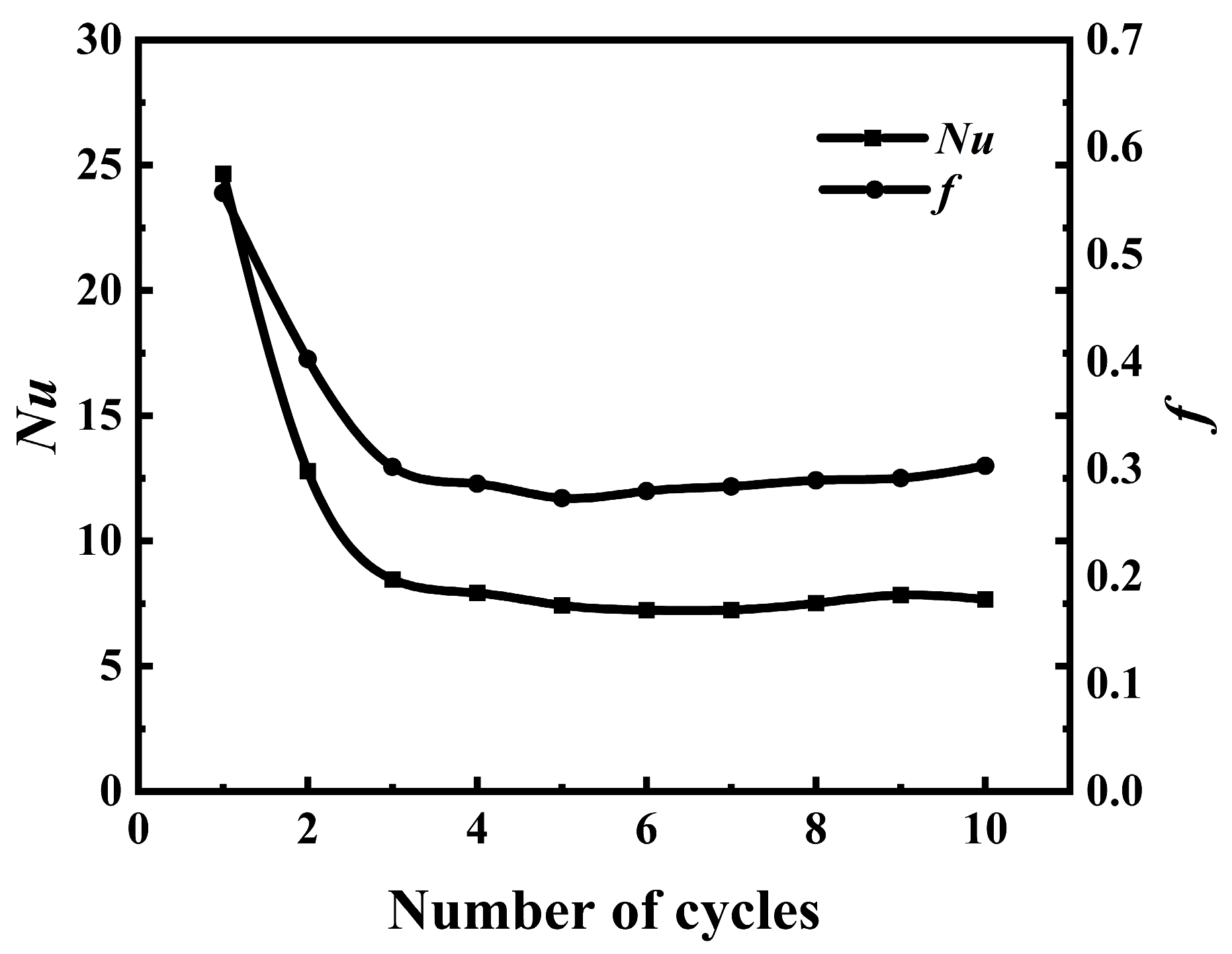
To determine the fully developed flow state of cross-corrugated triangular channels, we perform an initial model and simulation on a non-baffled channel with an apex angle of 60°. As depicted in Figure 4, the cell average Nu and f tend to stabilize after the fluid has passed through approximately four to five cycles. Therefore, we selected the average Nu and f for cells five to eight for discussion in this study.
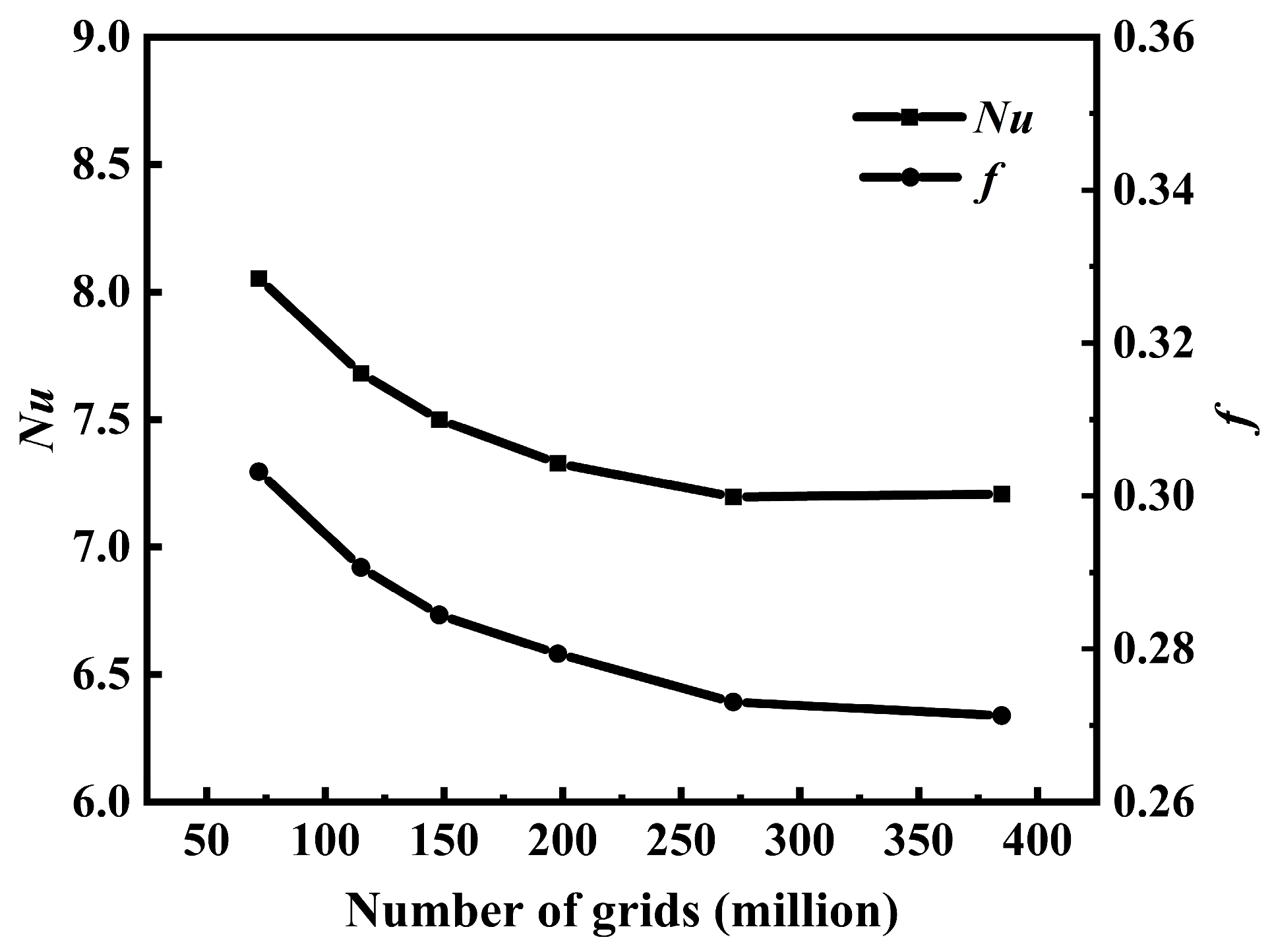
A tetrahedral mesh structure is used to partition the computational domain of the flow channel model. This choice is based on its better conformity to the flow channel geometry and improved mesh quality, as shown in Figure 5. To ensure the numerical solution is independent of the gid number, a grid-independent test is performed for each computational model. Theoretically, grid independence is achieved when further refinement of the computational grid cannot change the numerical solution. Examining the case of a 60° apex angle without baffles, Figure 6 shows the variations in the Nu and f corresponding to different numbers of grid cells. It is noticeable that the Nu and f remain approximately constant for cell numbers ranging from 2,716,585 to 3,851,163. Compared to a cell number of 3,851,163, there is a specific difference of 0.16% and 0.65% for Nu and f, respectively. This meets the requirements for computational simulation. Thus, grid size 2,716,585 is selected for the calculations due to its grid independence. Similar tests are carried out for other cases. The number for a flow channel with an apex angle of 90° is 1,919,626 and for a flow channel with an apex angle of 120° is 1,564,702.

3.5. Model Validation

To validate the numerical model, an experimental test rig with non-baffle cross-corrugated triangular ducts was conducted in this study. A photo of the experimental setup is shown in Figure 7. The experimental process is described in detail in the references [19,20]. Figure 8 shows the validation of the numerical model with the experimental data and reference data [33]. The maximum deviation between Nu and the comparison data is 11.9% and the f is 9.3%, both of which are within a reasonable range. It is worth noting that the largest errors appear at the lowest Reynolds number. This is due to the fact that the Reynolds Stress Model has a satisfactory simulation for the strong turbulence model [34], whereas, for low Re, the velocity is 1.1–1.6 m/s, which could be in a transition flow state [35]. The Reynolds Stress Model does not simulate transient flows effectively [36]. Overall, the data show good consistency, indicating that the mathematical model used is accurate.

4. Results and Discussion

4.1. ANOVA Parameter Modeling

The numerical simulation was performed using the parameter design geometry matrix listed in Table 2. The resulting data were collected and entered into a factorial design table to facilitate analysis of the response surface design fitted model.
In an ANOVA, Adj SS and Adj MS represent the adjusted sum of squares and adjusted mean square, respectively, both of which are used to measure the aberrance in the different components of the model. The F-value is the test statistic. It is used in models or terms to determine whether a term is associated with a response and in lack-of-fit terms to determine whether higher-order terms containing predictor variables are missing from the current model. A sufficiently large F-value indicates that the term or model is highly significant. The Adj SS, Adj MS, and F-values are used by Minitab to calculate the p-values of the terms. Decisions about the statistical significance of the terms and models are made from the p-values. The p-value represents the probability of rejecting the original hypothesis in a hypothesis test. If the p-value is less than or equal to the predefined significance level α, it indicates a statistically significant relationship between the response characteristics and the variable. Conversely, a p-value greater than α indicates non-significance. Usually, α is set at 0.05 [26]. The lack of fit concept in ANOVA is used to evaluate whether the chosen model effectively fits the data and can adequately account for differences between groups. In ANOVA, if the p-value from the lack of fit test is greater than the predetermined significance level (usually 0.05), then the hypothesis that the model adequately fits the data is not supported by sufficient evidence to be rejected. Conversely, if the p-value from the lack of fit test is less than the significance level, it indicates that the model is having difficulty explaining the data and may need to consider of a more complex model or other adjustments to better capture the variability present in the data.
Appendix A presents the ANOVA results of the quadratic model for Nu before elimination. The results indicate that some items are insignificant and can be removed. The lack of fit test also shows insignificance. Specifically, the main item X-direction position (C) is insignificant but its quadratic item is significant. Therefore, the main item X-direction position (C) is retained.
The insignificant terms were removed from the quadratic model for the Nu using a backward elimination process. Table 3 shows the resulting ANOVA data of the reduced quadratic model for the Nu. In Table 3, the main items’ apex angle (A), baffle angle (B), and Re (E), the squared items’ baffle angle (B * B), the squared items X-direction position (C * C), and the interaction item baffle angle * Re (B * E) all have p-values less than 0.05, indicating their significance. As the squared item for the X-direction position (C) is also significant, the main item X-direction position is retained. As the p-value for the lack of fit item is greater than 0.05, it indicates that the model does not have a significant lack of fit. Therefore, the second-order model is considered appropriate and there is no need for a more complicated model.
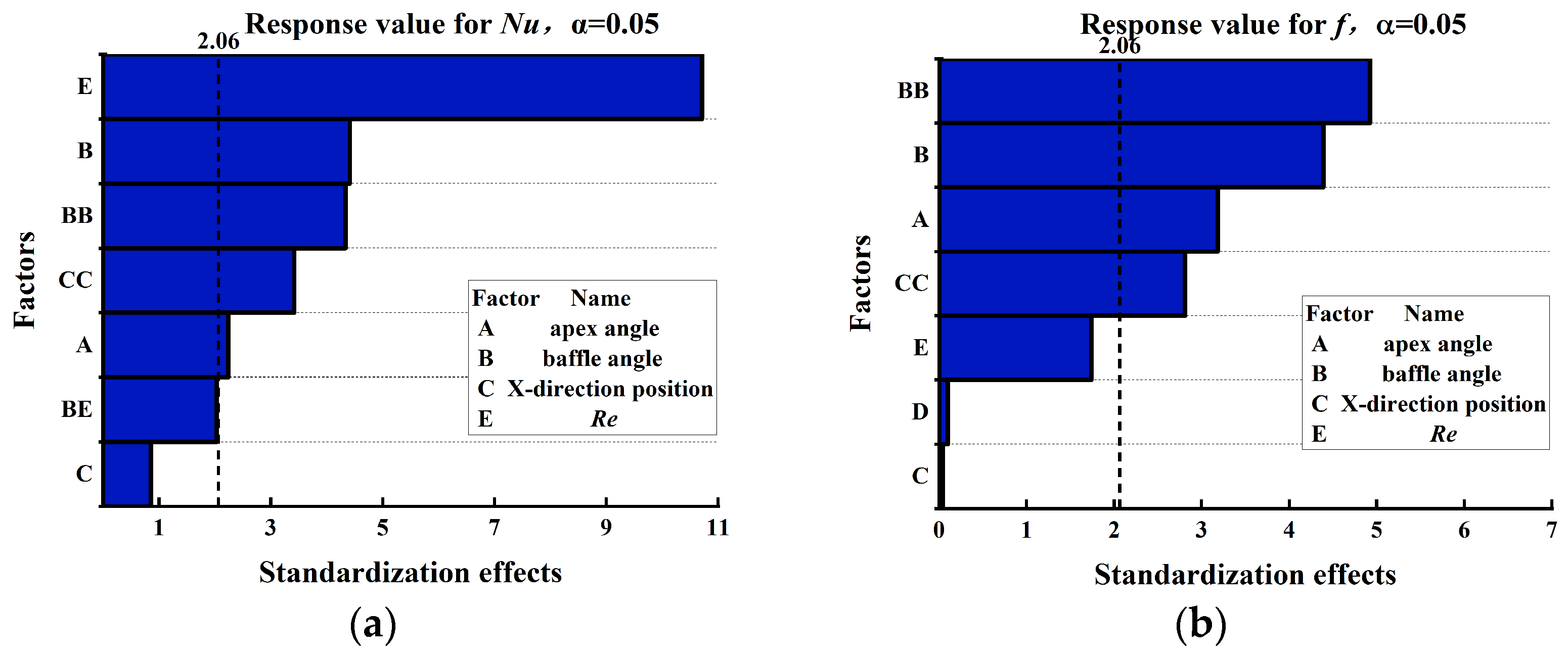
A Pareto standardization effect plot can provide more detailed insight into the relative influence of factors on the response variable, as well as their statistical significance, helping to identify influences that may have been missed in separate ANOVA tests [37]. The plot represents the effects of each factor with bar graphs, where the length of each bar indicates the magnitude of the influence on the response variable. Impact values are usually normalized for comparison purposes and a reference line is plotted on the graph, typically at a specific level of significance (e.g., 0.05). If the value of a factor in Figure 9 exceeds this threshold, it indicates that the factor is statistically significant. The greater the excess, the more significant the factor. Figure 9a depicts the Pareto chart of the standardization effects of the factors. It is observed that Re has the greatest influence on Nu, with a value more than twice that of the second most important factor. The other importance factors, in decreasing order of importance, are the baffle angle (B), quadratic items baffle angle (B * B), quadratic items X-direction position (C * C), apex angle (A), interaction item between baffle angle and the Re (B * E), and finally the X-direction position (C). Re indicates the state of fluid flow. The higher the Re, the greater the turbulence intensity, which has the greatest effect on the Nu. The angle and position of the baffle cause different degrees of fluid mixing between the center of the channel and the corrugated plate. It is important to note that Re reflects the state of the fluid flow, with a higher value indicating greater turbulence. As a result, the convective heat transfer coefficient will be greater, resulting in a stronger heat transfer capacity.
Appendix B presents the results of the quadratic model for f in the form of ANOVA before elimination. The main significant items for f, as shown in Appendix B, are the apex angle (A), baffle angle (B), quadratic items baffle angle (B * B), and quadratic items X-direction position (C * C). Table 4 shows the resulting ANOVA data of the reduced quadratic model for the f. It retains the main effect of the X-direction position (C) since its squared item is significant. In Appendix B, Re (E) is non-significant but removing it results in a p-value from the lack of fit test being less than the significance level. Table 4 shows that keeping Re results in a lack of fit greater than the significance level, indicating that the model does not lack fit. The Re is a turning point parameter and is therefore kept.
Furthermore, it has been discovered that the interaction between the baffle angle and Re is of significant importance. The baffle angle has the greatest impact on f, with the other factors decreasing progressively. This is due to the baffle causing the fluid to collide with the wall, resulting in energy loss and a variation in the pressure drop in the pipe. The second factor is the apex angle of the flow channel. In a flow channel with a small apex angle, the fluid flow is deflected more severely, resulting in greater energy dissipation and a greater pressure drop. The position of the channel also affects the disturbance of the upper and lower walls, which ultimately affects the f.
Based on the statistical analysis of the response results, the regression equation for the simulated data is determined using the following model:
N u = M X T M = 30.1 0.0438 0.432 89.5 0.00563 0.004099 73.2 0.00034 X = 1 A B C E B 2 C 2 B E
f = N Y T N = 0.561 0.002843 0.02423 3.43 0.000047 0.000201 2.737 Y = 1 A B C E B 2 C 2
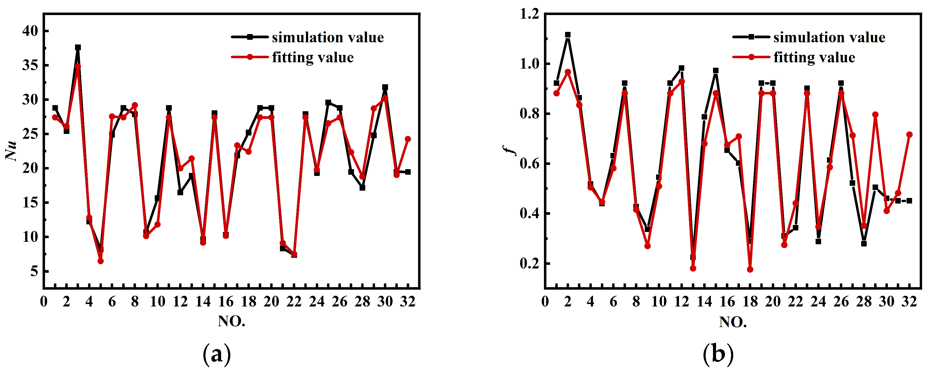
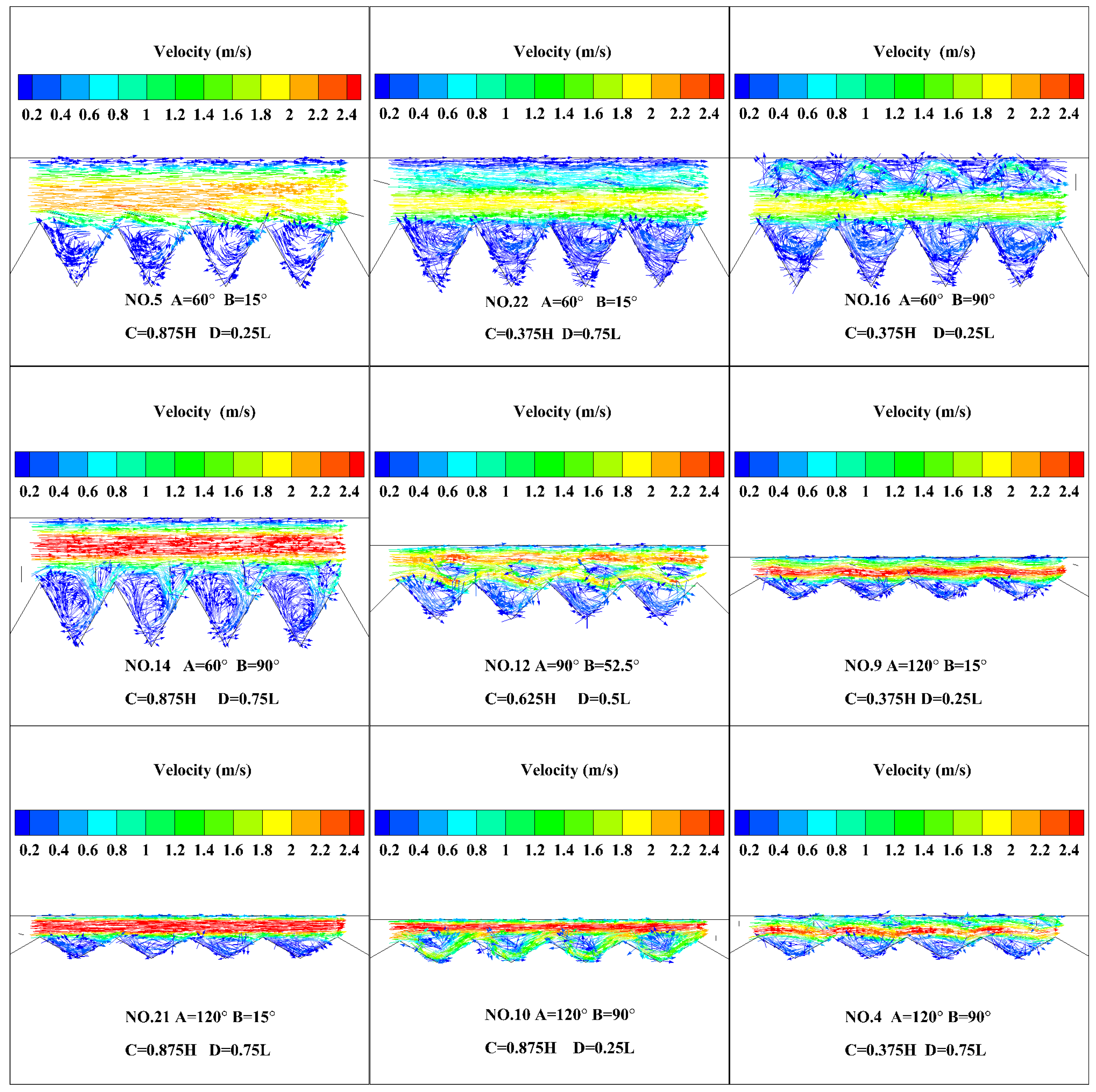
The sign in front of each item in the equation determines the effect of that item on a particular response. A positive sign indicates a synergistic effect, while a negative sign indicates an antagonistic effect. Within the range of values for each factor, the equation incorporates the actual value to calculate the corresponding response value. The 32 groups of simulation conditions were taken into the regression equation for comparison and validation; the results are shown in Figure 10. For Nu, the root mean square error (RMSE) of the model is 2.081. The smaller the value and closer it is to two, the more acceptable the value. A group of outlier observations exists at NO.32. For f, the RMSE of the model is 0.098. Three groups of outlier observations exist at NO.27, NO.29, and NO.32. In general, the regression equations for Nu are better than f and this result corresponds to Table 5. Due to the finite degree of fit, they are the optimal model that can be reached. For the cross-corrugated triangular plate heat exchangers with interpolated trapezoidal in this study range, the regression equation is able to predict the simulated values relatively accurately in the majority of scenarios. It could provide guidelines for the design and optimization of cross-corrugated triangular flow channels under non-standard conditions. Moreover, further observations were made by choosing the same Re (1000) cases in 32 groups of models for the nine NO.4, NO.5, NO.9, NO.10, NO.12, NO.14, NO.16, NO.21, and NO.22 values, respectively.
The model summary in Table 5 confirms the fitting results. ‘S’ represents the standard deviation of the distance between the data values and the fitted values; the lower the ‘S’ value, the better the model describes the response value. ‘R-sq’ is used to determine how well the model fits the data. The higher the ‘R-sq’ value, the better the model fits the data. The ‘R-sq’ (Adjustment) is the ratio of the number of predictor variables. In cases where you want to compare variables with different numbers of predictors, using the ‘R-sq’ (Adjustment) when comparing variables with different numbers of predictors. The ‘R-sq’ (Projections) measures the extent to which the model predicts the response to new observations. Models with higher predictive ‘R-sq’ values have better predictive ability. In this model, the goodness of fit statistic R-sq, R-sq (Adjustment) and R-sq (Projections) for Nu are all close to 1, indicating a goodness of fit to the simulated data. The results for f are also good, although not as strong as for Nu.

4.2. Analysis of Factors

Figure 11 and Figure 12 show the main effects of Nu and f, respectively, indicating the impact of individual factors on the observed trends. A horizontal line (parallel to the X-axis), indicates no main effect, while a steeper line indicates a greater magnitude of the main effect. Figure 11 depicts an effect plot of the Nu. It is clear that the baffle angle and X-direction position factors exhibit a bend in the examined range, reaching a maximum at the top of their parabola, especially at 65° and 0.612H, respectively. The relationship between the factor of apex angle, Re, and Nu is linear, with a maximum at 120° and 3000. Cross-corrugated triangular ducts exhibit superior heat transfer performance under these conditions, with a corresponding Nu fitting value of 36.78. The results were verified by simulation to be 36.54. This value is 1.54 times that of a non-baffled channel with the same apex angle and Re. Figure 12 shows an effect plot of the f. The baffle angle and X-direction position factors reach their minimum values at 15° and 0.875H, respectively. The apex angle and Re factors are linearly related to f, reaching their minimum values at their rightmost points, 120° and 3000, respectively, with corresponding f fitting values of 0.181. The results were verified by simulation to be 0.225. This value is close to the non-baffled channel and even lower than it by 0.007 with the same apex angle and Re.
When optimizing the performance of cross-corrugated triangular ducts, it is desirable to maximize Nu and minimize f. The response prediction value suggests that the optimal model has an apex angle of 90°, a baffle angle of 52.5°, and a distance of 0.625H in the X-direction with a Re number of 1000. It is important to maintain a balance between Nu and f to achieve optimum performance. At this point, the value of Nu is 16.45 and f is 0.98, resulting in a calculated PEC of 1.22. This represents a significant improvement compared to the case over no baffle.
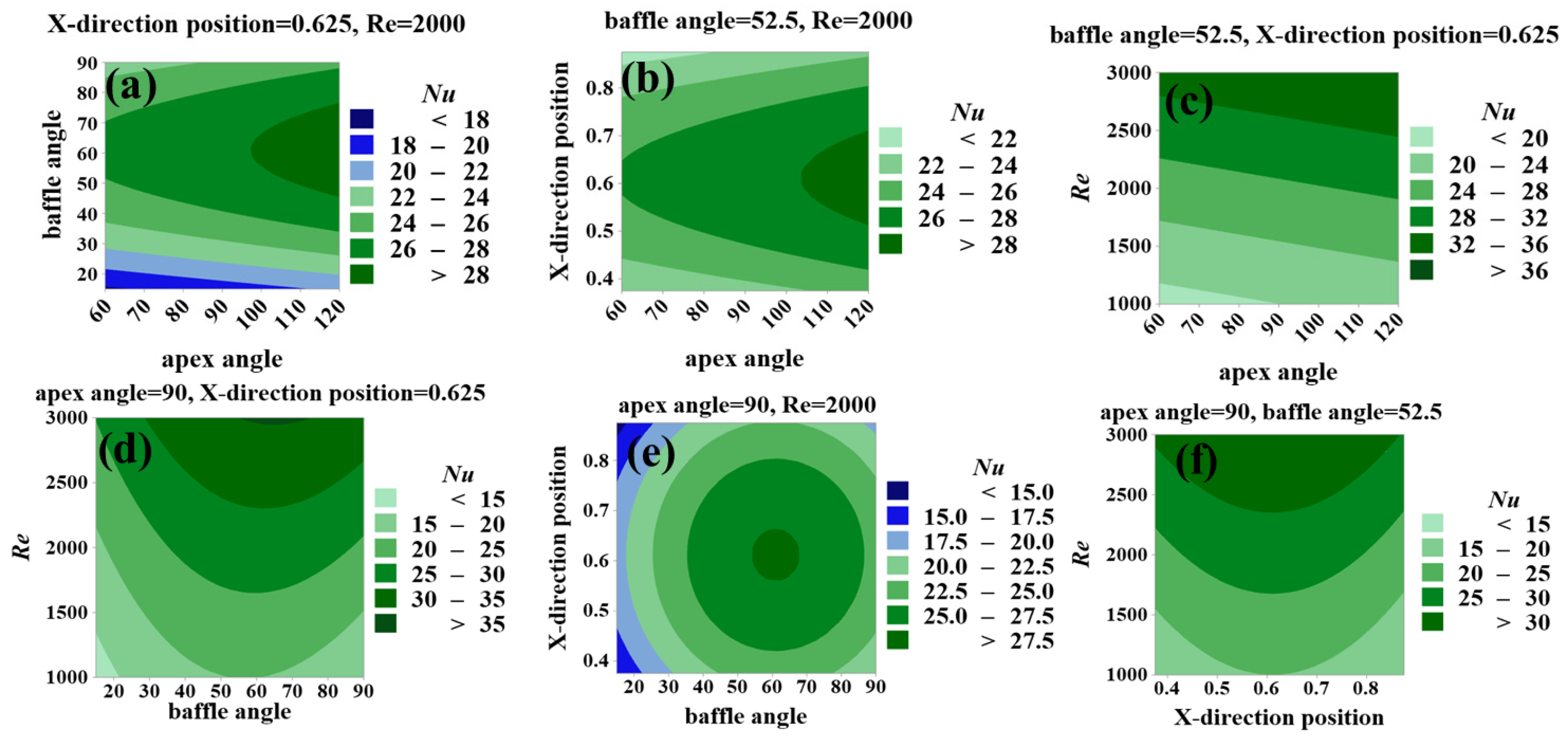
Figure 13 shows a contour plot of Nu against each factor, allowing for exploration of the desired response values and operating conditions. The plot illustrates the relationship between the two significant predictor variables and the response variable Nu. The darker colors indicate higher values and better quality. Using the interaction between the apex angle and baffle angle as an example (see Figure 13a) and holding the other variables constant, Nu is expected to be above 28 for an apex angle greater than 98° and a baffle angle between 46° and 80°. Conversely, when the apex angle is between 60° and 110° and the baffle angle is less than 22°, Nu is just below 18, which is a difference of 1.6 times in the results. The remaining part of the Nu plot exhibits differences ranging from 1.3 to 2.3 times. Figure 14 shows a plot of the contours f against each factor. To ensure the smallest possible expected value of f, the optimal range for f is limited to the light green and blue areas. For example, when considering the interaction between the apex angle and baffle angle (see Figure 14a), while holding the other variables constant, f should be less than 0.4 when the apex angle is between 85° and 120° and the baffle angle is less than 20°. Conversely, when the apex angle is between 60° and 85° and the baffle angle is 40° and 80°, f should be over 0.9, which represents a difference of 2.3 times in the results. The remainder of the f plot also exhibits a difference ranging from 1.5 to 2.0 times.
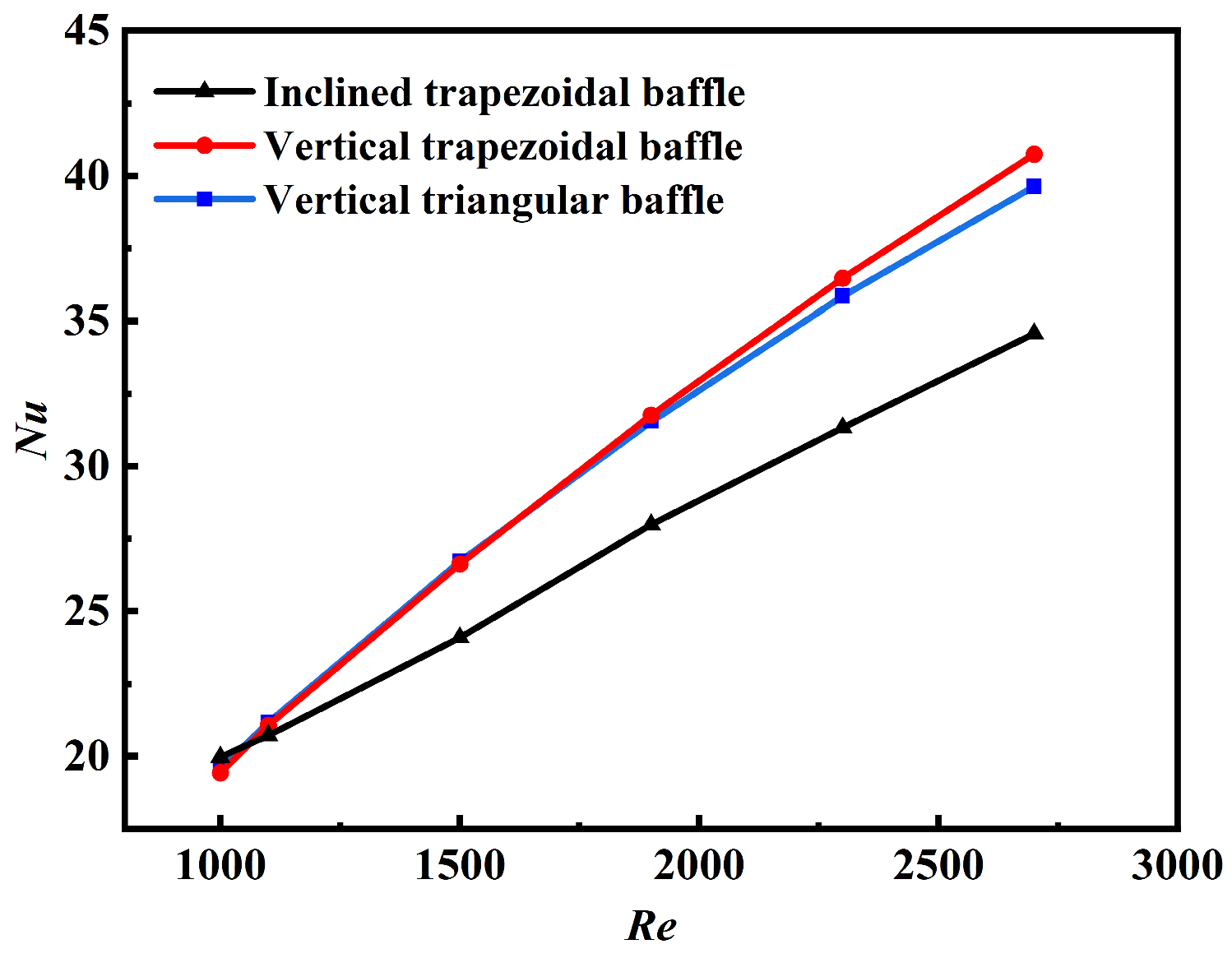
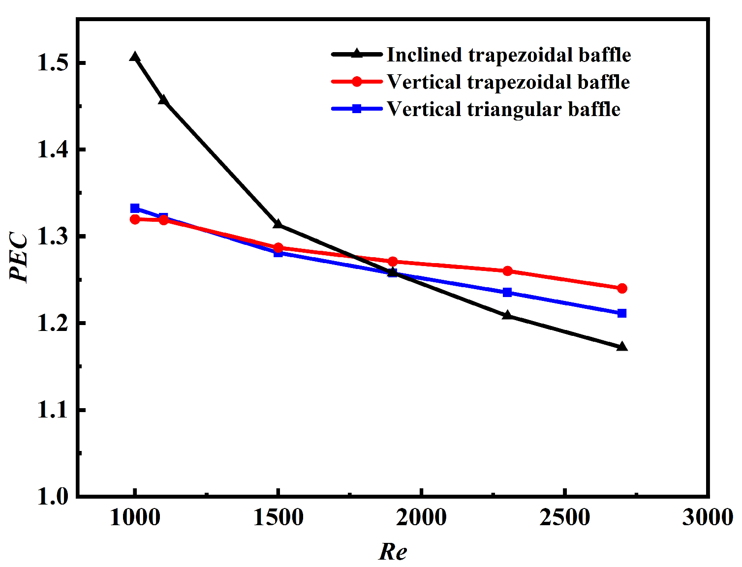
To visualize the influence of the baffle inclination on the heat transfer and pressure drop characteristics, a comparison is made with the existing vertical trapezoidal and triangular baffles under the conditions of the geometry with the best comprehensive performance (apex angle of 90°, baffle inclination angle of 52.5°, baffle positions of 0.625H and 0.5L). The Re was chosen for the range of overlap (1000–2700). Figure 15 and Figure 16 show the comparison results for Nu and f, respectively. It can be seen from the figure that the inclined baffle attenuates both Nu and f compared to the vertical baffle, while the comprehensive performance needs to be judged from Figure 17. A significant increase in PEC can be observed for the inclined baffle at low Re. This is because the inclined baffle has a minor difference in Nu compared to the vertical baffle, while f is far less than that of the vertical baffle. As the Re increases, the increase in PEC is no longer evident. As soon as the intersection point (near 1750) is exceeded, the comprehensive performance is lower than that of the vertical baffle. Thereafter, the gap in Nu gradually becomes wider, while the change in f is slight, so the performance is below that of the vertical baffle. Furthermore, it is observed that the trapezoidal baffle is generally ahead of the triangular baffle.

4.3. Velocity Field Distribution

Figure 18 shows the velocity field distribution from the fifth to the eighth fluid cell at a Re of 1000. For NO.5, it is evident that when the baffle is in the lower half and inclined at 15°, the fluid in the upper half flows through the channel in an advective manner with minimal disturbance. A slight disturbance is only observed near the corrugated groove, where a clockwise vortex appears in the groove. By placing the same baffle on the upper part of the NO.22 channel, it reduces the flow rate of the upper fluid and causes more fluid to flow to the lower part. Although more vortices are generated at the corrugation, the speed is not as high as before. In NO.16, when the baffle is inclined 90°, vortices become visible at the rear of the baffle. The density of vortices in the slot increases and the collision between the fluid and the baffle intensifies, resulting in more adequate mixing. This results in a notable rise in pressure difference, which subsequently increases f, making it more probable for vortices to form at larger baffle angles. When the baffle is located in the lower half, a significant backflow phenomenon arises in the NO.14 slot, with some of the fluid flowing back to the front through the gap between the baffle and the slot. The flow patterns of models with 90 and 120° apex angles are similar to those of the 60°.
The computation shows that the highest PEC value among the nine cases is NO.12 with 1.22, followed by NO.10 with 1.21. It is obvious that both cases have significant vortices in the channel. In NO.12, the baffle is positioned in the center, with a larger area. This results in a uniform discharge of fluid in both the upper and lower parts of the flow channel, which produces noticeable vortices on the lower wall surface of the groove. The gas rotates along the groove wall, effectively promoting the mixing of the middle and bottom fluid. This intensifies the internal friction and collision of the fluid, thus increasing energy consumption. The most optimal gas separation results are achieved at this junction. In NO.10, the channel height is at its minimum and the vertically oriented baffle accelerates the fluid flow in its vicinity, resulting in a greater dependence of heat transfer on particle movement and a thinner hydrodynamic and thermal boundary. Additionally, the vortices created disturbances in the boundary layer, further thinning it.

4.4. Temperature Distribution

Figure 19 shows some cloud plots of the temperature distribution under the same conditions. It is evident from NO.5, NO.22, and NO.16 that the position and angle of the baffle have a significant effect on the gradient of the thermal boundary layer. Particularly, when the baffle is placed at a lower position and small angle, the thermal boundary layer gradient increases at the lower wall, while it has almost no effect on the upper wall. Conversely, when the baffle is placed at the upper part, the situation is reversed. Due to the high position of the baffle, the return flow is too close to the thermal boundary layer, which is detrimental to heat transfer and may cause excessive energy loss. Compared with NO.16, the larger baffle angle causes more disturbance to the upper boundary layer, making it relatively optimal. NO.14 places the baffle near the corrugated groove, which increases the uneven temperature distribution in the groove, but the average temperature in the center is not as high as the former. Models with 90 and 120° apex angles have a thinner thermal boundary layer compared to 60° and are affected by the baffle in a similar pattern.
It is evident that NO.12 and NO.10 exhibit excellent overall performance, due to their uniform temperature distribution in the central channel and high average temperature, resulting in better heat transfer performance.

5. Conclusions

This paper utilizes the factorial design method of response surfaces and numerical computations to investigate the fluid flow and heat transfer performance of cross-corrugated triangular ducts with interpolated trapezoidal baffles. The study examines the impact of five factors: apex angle, baffle angle, X-direction position, Y-direction position, and Re. The main conclusions are presented below.
  • When the response value is Nu, the four factors that have a significant influence are the apex angle, baffle angle, X-direction position, and Re. The factor with the greatest influence factor is Re, which exceeds the other factors by more than two times. Nu rises linearly with the increase in Re. The factors baffle angle and X-direction position have a parabolic relationship with Nu. As these factors increase, Nu first increases and then decreases. Compared to these three factors, the effect of the apex angle factor is smaller and slightly increases with increasing Re. The best heat transfer performance of the model is achieved when optimized for maximum Nu, with a factor apex angle of 120°, baffle angle of 65°, X-direction position of 0.612H, and Re of 3000. Under the same apex angle and Re conditions, Nu values are 1.54 times that of a non-baffled channel;
  • If the response value is f, the four factors that have a significant effect are the apex angle, baffle angle, X-direction position, and Re. The baffle angle has the largest effect, while the others gradually decrease. The baffle angle and X-direction position exhibit a parabolic trend, increasing and then decreasing, while the apex angle and Re show a negative linear relationship with f. The value of f decreases slowly as the apex angle and Re increase. When optimized for minimum f, the factor apex angle is 120°, baffle angle is 15°, X-direction position is 0.875H, and Re is 3000. Under these conditions, the pressure drop of the model is minimized. This value is close to the non-baffled channel and even lower than it by 0.007 with the same apex angle and Re;
  • The optimal PEC was found to be 90° for the factor apex angle, 52.5° for the baffle angle, 0.625H for the X-direction position, and 1000 for Re. The inclined baffle significantly outperforms the vertical baffle at low Re and this is no longer obvious as the Re increases.
In conclusion, the combination of response surface methodology and CFD provides a valuable reference for researchers and manufacturers to optimize and manufacture heat transfer equipment. It serves as a guide for the design and optimization of cross-corrugated triangular ducts, significantly reducing time and economic costs. Further research will be devoted to exploring the design of perforated baffles and the economics of heat exchangers.

Author Contributions

Conceptualization, C.L. and C.M.; methodology W.H.; software, R.Z.; validation, Y.D. and Z.L.; formal analysis, X.Y.; investigation, R.Z.; resources, Y.D.; data curation, X.Y.; writing—original draft preparation, R.Z.; writing—review and editing, C.L. and Z.L.; visualization, R.Z.; supervision, C.L.; project administration, W.H.; funding acquisition, C.L. All authors have read and agreed to the published version of the manuscript.

Funding

The study was supported by the Natural Science Foundation of China (Grant No. 51566002), Guangxi Science and Technology Plan Project (Grant No. AB23075143), Innovation Project of Guang Xi Graduate Education (Grant No. YCSW2023299).

Data Availability Statement

The original contributions presented in the study are included in the article, further inquiries can be directed to the corresponding authors.

Conflicts of Interest

The authors declare no conflicts of interest.

Nomenclature

Symbols
AciCross-sectional area at inlet or outlet, m2
AcycSurface area of a cycle, m2
cpSpecific heat of the fluid, kJ/(kg·K)
DhHydraulic diameter of the channel, m
fFriction factor
HCorrugation height of a cycle, m
hConvective heat transfer coefficient, W/(m2·K)
LCorrugation length of a cycle, m
NNumber of trials
NuNusselt number
PPressure, Pa
PECPerformance Evaluation Criteria
PrPrandtl number
ReReynold number
R-sqDegree of fitting
SStandard deviation
TTemperature, °C
TmLogarithmic mean temperature, °C
uVelocity, m/s
Vcycvolume of a cycle, m3
Wcorrugation width of a cycle, m
x, y, zcoordinates, m
Greek letters
σerror term
ρdensity, kg/m3
Superscripts
*dimensionless
Subscripts
i, oinlet and outlet
wwall
mmean value
0unbaffled channel
bulk flow
Codes
Aapex angle (°)
Bbaffle angle (°)
CX-direction position
DY-direction position
ERe

Appendix A. ANOVA for Nu before Elimination

SourceDegree of FreedomAdj SSAdj MSF-Valuep-Value
Model 201972.1198.60612.980.000
Linear 51153.60230.71930.380.000
A131.1131.1114.100.068
B1121.57121.56616.010.002
C14.474.4670.590.459
D17.347.3360.970.347
E1989.12989.116130.240.000
Square 5750.60150.11919.770.000
A * A12.242.2390.290.598
B * B1106.80106.79814.060.003
C * C171.7071.7049.440.011
D * D18.978.9681.180.300
E * E12.322.3210.310.591
Two-factor interaction 1067.926.7920.890.566
A * B10.250.2450.030.861
A * C18.928.9221.170.302
A * D11.511.5060.200.665
A * E10.140.1350.020.896
B * C111.4811.4761.510.245
B * D111.4811.4781.510.245
B * E125.8525.8473.400.092
C * D12.902.8970.380.549
C * E14.954.9520.650.436
D * E10.460.4600.060.810
Residual 1183.547.594--
Lack of Fit674.9612.4947.290.023
Pure Error58.571.715--
Total 312055.65---

Appendix B. ANOVA for f before Elimination

SourceDegree of FreedomAdj SSAdj MSF-Valuep-Value
Model 201.967700.0983855.300.003
Linear 50.421740.0843484.550.017
A10.130970.1309697.060.022
B10.251300.25130213.540.004
C10.000040.0000360.000.966
D10.000500.0004960.030.873
E10.038940.0389372.100.175
Square 51.509970.30199516.280.000
A * A10.000290.0002920.020.902
B * B10.338340.33833618.240.001
C* C10.165820.1658198.940.012
D * D10.033230.0332311.790.208
E * E10.025530.0255321.380.266
Two-factor interaction 100.035980.0035980.190.992
A * B10.018690.0186911.010.337
A * C10.005620.0056150.300.593
A * D10.000280.0002830.020.904
A * E10.000650.0006460.030.855
B * C10.000780.0007810.040.841
B * D10.001560.0015610.080.777
B * E10.000030.0000320.000.968
C * D10.000230.0002340.010.913
C * E10.007930.0079300.430.527
D * E10.000210.0002110.010.917
Residual 110.204090.018553--
Lack of Fit60.186160.0310268.650.016
Pure Error50.017930.003586--
Total 312.17179- --

References

  1. Agency, I.E. World Energy Outlook 2023. Available online: https://origin.iea.org/reports/world-energy-outlook-2023 (accessed on 21 November 2023).
  2. Zukowski, M.; Topolanska, J. Comparison of Thermal Performance between Tube and Plate Ground-Air Heat Exchangers. Renew. Energy 2018, 115, 697–710. [Google Scholar] [CrossRef]
  3. García-Castillo, J.L.; Picón-Núñez, M.; Abu-Khader, M.M. Improving the Prediction of the Thermohydraulic Performance of Secondary Surfaces and Its Application in Heat Recovery Processes. Energy 2022, 261, 125196. [Google Scholar] [CrossRef]
  4. Chennu, R. Numerical Analysis of Compact Plate-Fin Heat Exchangers for Aerospace Applications. HFF 2018, 28, 395–412. [Google Scholar] [CrossRef]
  5. Aneesh, A.M.; Sharma, A.; Srivastava, A.; Chaudhury, P. Effects of Wavy Channel Configurations on Thermal-Hydraulic Characteristics of Printed Circuit Heat Exchanger (PCHE). Int. J. Heat Mass Transf. 2018, 118, 304–315. [Google Scholar] [CrossRef]
  6. Zhang, L.; Che, D. Influence of Corrugation Profile on the Thermalhydraulic Performance of Cross-Corrugated Plates. Numer. Heat Transf. Part A Appl. 2011, 59, 267–296. [Google Scholar] [CrossRef]
  7. Liao, J.; Xue, P.; Jin, L.; Zhao, M.; Zhang, N.; Liu, J. Optimization of Corrugated Sheet Packing Structure Based on Analysis of Falling Film Flow Characteristics. Sustainability 2022, 14, 5861. [Google Scholar] [CrossRef]
  8. Younis, O.; Abderrahmane, A.; Hatami, M.; Mourad, A.; Kamel, G. Thermal Energy Storage Using Nano Phase Change Materials in Corrugated Plates Heat Exchangers with Different Geometries. J. Energy Storage 2022, 55, 105785. [Google Scholar] [CrossRef]
  9. Verdério Júnior, S.A.; Coelho, P.J.; Scalon, V.L.; Del Rio Oliveira, S. Numerical and Experimental Study of Natural Convection Heat Transfer on Flat and Corrugated Plates. HFF 2023, 33, 3286–3307. [Google Scholar] [CrossRef]
  10. Krishnan, E.N.; Ramin, H.; Guruabalan, A.; Simonson, C.J. Experimental Investigation on Thermo-Hydraulic Performance of Triangular Cross-Corrugated Flow Passages. Int. Commun. Heat Mass Transf. 2021, 122, 105160. [Google Scholar] [CrossRef]
  11. Sarraf, K.; Launay, S.; Tadrist, L. Complex 3D-Flow Analysis and Corrugation Angle Effect in Plate Heat Exchangers. Int. J. Therm. Sci. 2015, 94, 126–138. [Google Scholar] [CrossRef]
  12. Cao, X.; Chen, D.; Du, T.; Liu, Z.; Ji, S. Numerical Investigation and Experimental Validation of Thermo-Hydraulic and Thermodynamic Performances of Helical Baffle Heat Exchangers with Different Baffle Configurations. Int. J. Heat Mass Transf. 2020, 160, 120181. [Google Scholar] [CrossRef]
  13. Handoyo, E.A.; Ichsani, D.; Prabowo; Sutardi. Numerical Studies on the Effect of Delta-Shaped Obstacles’ Spacing on the Heat Transfer and Pressure Drop in v-Corrugated Channel of Solar Air Heater. Sol. Energy 2016, 131, 47–60. [Google Scholar] [CrossRef]
  14. Karabulut, K. Heat Transfer and Pressure Drop Evaluation of Different Triangular Baffle Placement Angles in Cross-Corrugated Triangular Channels. Therm. Sci. 2020, 24 Pt A, 355–365. [Google Scholar] [CrossRef]
  15. Alnak, D.E. Thermohydraulic Performance Study of Different Square Baffle Angles in Cross-Corrugated Channel. J. Energy Storage 2020, 28, 101295. [Google Scholar] [CrossRef]
  16. Akcay, S. Numerical Analysis of Heat Transfer Improvement for Pulsating Flow in a Periodic Corrugated Channel with Discrete V-Type Winglets. Int. Commun. Heat Mass Transf. 2022, 134, 105991. [Google Scholar] [CrossRef]
  17. Akcay, S.; Akdag, U. Heat Transfer Enhancement in a Channel with Inclined Baffles under Pulsating Flow: A Cfd Study. J. Enhanc. Heat Transf. 2023, 30, 61–79. [Google Scholar] [CrossRef]
  18. Liang, C.; Tong, X.; Lei, T.; Li, Z.; Wu, G. Optimal Design of an Air-to-Air Heat Exchanger with Cross-Corrugated Triangular Ducts by Using a Particle Swarm Optimization Algorithm. Appl. Sci. 2017, 7, 554. [Google Scholar] [CrossRef]
  19. Feng, C.-N.; Liang, C.-H.; Li, Z.-X. Friction Factor and Heat Transfer Evaluation of Cross-Corrugated Triangular Flow Channels with Trapezoidal Baffles. Energy Build. 2022, 257, 111816. [Google Scholar] [CrossRef]
  20. Li, Z.-X.; Sun, S.-Q.; Wang, C.; Liang, C.-H.; Zeng, S.; Zhong, T.; Hu, W.-P.; Feng, C.-N. The Effect of Trapezoidal Baffles on Heat and Flow Characteristics of a Cross-Corrugated Triangular Duct. Case Stud. Therm. Eng. 2022, 33, 101903. [Google Scholar] [CrossRef]
  21. Atkinson, A.C. Optimum and Other Response Surface Designs. Comments on “Response Surface Design Evaluation and Comparison” by Anderson-Cook, Borror and Montgomery. J. Stat. Plan. Inference 2009, 139, 662–668. [Google Scholar] [CrossRef]
  22. Sharma, R.; Mishra, D.P.; Wasilewski, M.; Brar, L.S. Application of Response Surface Methodology and Artificial Neural Network to Optimize the Curved Trapezoidal Winglet Geometry for Enhancing the Performance of a Fin-and-Tube Heat Exchanger. Energies 2023, 16, 4209. [Google Scholar] [CrossRef]
  23. Yu, C.; Chen, J.; Zeng, M.; Gao, B. Numerical Study on Turbulent Heat Transfer Performance of a New Parallel-Flow Shell and Tube Heat Exchanger with Sinusoidal Wavy Tapes Using RSM Analysis. Appl. Therm. Eng. 2019, 150, 875–887. [Google Scholar] [CrossRef]
  24. Kola, P.V.K.V.; Pisipaty, S.K.; Mendu, S.S.; Ghosh, R. Optimization of Performance Parameters of a Double Pipe Heat Exchanger with Cut Twisted Tapes Using CFD and RSM. Chem. Eng. Process. Process Intensif. 2021, 163, 108362. [Google Scholar] [CrossRef]
  25. Rezaei, P.; Moheghi, H.R.; Amiri Delouei, A. Design and Optimization of a Spiral-Tube Instantaneous Water Heater Using Response Surface Methodology. Water 2023, 15, 1458. [Google Scholar] [CrossRef]
  26. Support|Minitab. Available online: https://www.minitab.com/ (accessed on 3 June 2023).
  27. Zhang, L. Convective Mass Transport in Cross-Corrugated Membrane Exchangers. J. Membr. Sci. 2005, 260, 75–83. [Google Scholar] [CrossRef]
  28. Bahiraei, M.; Mazaheri, N.; Hanooni, M. Employing a Novel Crimped-Spiral Rib inside a Triple-Tube Heat Exchanger Working with a Nanofluid for Solar Thermal Applications: Irreversibility Characteristics. Sustain. Energy Technol. Assess. 2022, 52, 102080. [Google Scholar] [CrossRef]
  29. Močnik, U.; Muhič, S. Experimental and Numerical Analysis of Heat Transfer in a Dimple Pattern Heat Exchanger Channel. Appl. Therm. Eng. 2023, 230, 120865. [Google Scholar] [CrossRef]
  30. Liu, X.P.; Niu, J.L. Effects of Geometrical Parameters on the Thermohydraulic Characteristics of Periodic Cross-Corrugated Channels. Int. J. Heat Mass Transf. 2015, 84, 542–549. [Google Scholar] [CrossRef]
  31. Sharif, A.; Ameel, B.; T’Jollyn, I.; Lecompte, S.; De Paepe, M. Comparative Performance Assessment of Plate Heat Exchangers with Triangular Corrugation. Appl. Therm. Eng. 2018, 141, 186–199. [Google Scholar] [CrossRef]
  32. Ansys|Engineering Simulation Software. Available online: https://www.ansys.com/ (accessed on 13 August 2023).
  33. Li, Z.; Gao, Y. Numerical Study of Turbulent Flow and Heat Transfer in Cross-Corrugated Triangular Ducts with Delta-Shaped Baffles. Int. J. Heat Mass Transf. 2017, 108, 658–670. [Google Scholar] [CrossRef]
  34. Tian, L.; Song, Y.; Zhao, N.; Shen, W.; Wang, T. AD/RANS Simulations of Wind Turbine Wake Flow Employing the RSM Turbulence Model: Impact of Isotropic and Anisotropic Inflow Conditions. Energies 2019, 12, 4026. [Google Scholar] [CrossRef]
  35. Peng, H.; Ling, X.; Li, J. Performance Investigation of an Innovative Offset Strip Fin Arrays in Compact Heat Exchangers. Energy Convers. Manag. 2014, 80, 287–297. [Google Scholar] [CrossRef]
  36. Liu, Y.; Luo, P.; Tang, Y. Improved Prediction of Turbomachinery Flows Using Reynolds Stress Model with γ Transition Model. Aerosp. Sci. Technol. 2024, 144, 108812. [Google Scholar] [CrossRef]
  37. Parekh, J.; Rzehak, R. Euler–Euler Multiphase CFD-Simulation with Full Reynolds Stress Model and Anisotropic Bubble-Induced Turbulence. Int. J. Multiph. Flow 2018, 99, 231–245. [Google Scholar] [CrossRef]
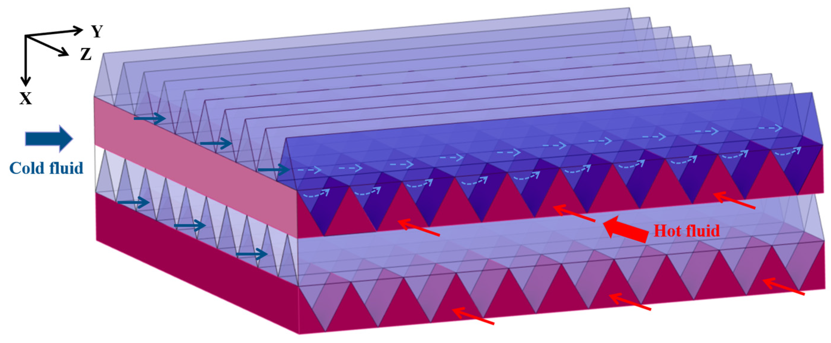
Figure 1. Schematic of the cross-corrugated triangular heat exchanger.
Energies 17 02335 g001
Figure 2. Geometry and baffle position of the unit channel corresponding to the factor level. (a) Apex angle; (b) Baffle angle; (c) X-position; (d) Y-position.
Energies 17 02335 g002
Figure 3. Geometry.
Figure 3. Geometry.
Energies 17 02335 g003
Figure 4. Computation cycle.
Energies 17 02335 g004
Figure 5. Segment of the computational grid.
Energies 17 02335 g005
Figure 6. Grid-independent verification.
Energies 17 02335 g006
Figure 7. Experimental setup.
Energies 17 02335 g007
Figure 8. Validation of the numerical model with the experimental data and reference [33] data. (a) Comparison of Nu (NON-60). (b) Comparison of f (NON-60).
Energies 17 02335 g008
Figure 9. Pareto of the standardization effects of the factors. (a) Nu. (b) f.
Energies 17 02335 g009
Figure 10. Comparison of simulation and fitting values. (a) Nu. (b) f.
Energies 17 02335 g010
Figure 11. The effects of the apex angle, baffle angle, X-direction position, and Re on Nu.
Energies 17 02335 g011
Figure 12. The effects of the apex angle, baffle angle, X-direction position, and Re on f.
Energies 17 02335 g012
Figure 13. Nu two-factor interaction contour plot. (a) apex angle and baffle angle. (b) apex angle and X-direction position. (c) apex angle and Re. (d) baffle angle and Re. (e) baffle angle and X-direction position. (f) X-direction position and Re.
Energies 17 02335 g013
Figure 14. f two-factor interaction contour plot. (a) apex angle and baffle angle. (b) apex angle and X-direction position. (c) baffle angle and X-direction position.
Energies 17 02335 g014
Figure 15. Comparison of Nu for inclined trapezoidal baffle with vertical trapezoidal baffle [19] and vertical triangular baffle [20].
Energies 17 02335 g015
Figure 16. Comparison of f for inclined trapezoidal baffle with vertical trapezoidal baffle [19] and vertical triangular baffle [20].
Energies 17 02335 g016
Figure 17. Comparison of PEC for inclined trapezoidal baffle with vertical trapezoidal baffle [19] and vertical triangular baffle [20].
Energies 17 02335 g017
Figure 18. Velocity field distribution for 9 typical cases.
Energies 17 02335 g018
Figure 19. Temperature distribution for 9 typical cases.
Energies 17 02335 g019
Table 1. Factors and levels for the central composite design.
Factors CodesLevels
−101
apex angle (°)A6090120
baffle angle (°)B1552.590
X-direction position C0.375H0.625H0.875H
Y-direction positionD0.25L0.5L0.75L
ReE100020003000
Table 2. Design geometry matrix.
RunLevelsFactorsResponse Values
Apex
Angle (°)
Baffle
Angle (°)
X-Direction PositionY-Direction PositionReNuf
109052.50.625H0.50L200028.805 0.922
2−16052.50.625H0.50L200025.414 1.116
3−19052.50.625H0.50L300037.602 0.864
4112090.00.375H0.75L100012.250 0.518
516015.00.875H0.25L10008.177 0.439
616090.00.375H0.75L300024.888 0.632
709052.50.625H0.50L200028.805 0.922
8112090.00.875H0.75L300027.880 0.427
9112015.00.375H0.25100010.717 0.337
10112090.00.875H0.25L100015.615 0.545
1109052.50.625H0.50L200028.805 0.922
12−19052.50.625H0.50L100016.452 0.983
13112015.00.875H0.25L300018.899 0.225
1416090.00.875H0.75L10009.673 0.787
15−19052.50.625H0.75L200028.028 0.973
1616090.00.375H0.25L100010.291 0.654
17−19052.50.375H0.50L200021.864 0.602
18112015.00.375H0.75L300025.213 0.289
1909052.50.625H0.50L200028.805 0.922
2009052.50.625H0.50L200028.805 0.922
21112015.00.875H0.75L10008.339 0.310
2216015.00.375H0.75L10007.372 0.342
23−19052.50.625H0.25L200027.901 0.902
2416015.00.375H0.25L300019.315 0.288
2516090.00.875H0.25L300029.564 0.614
2609052.50.625H0.50L200028.805 0.922
27−19052.50.875H0.50L200019.451 0.521
2816015.00.875H0.75L300017.150 0.279
29−112052.50.625H0.50L200024.790 0.504
30112090.00.375H0.25L300031.805 0.460
31−19015.00.625H0.50L200019.471 0.450
32−19090.00.625H0.50L200019.465 0.451
Table 3. ANOVA for Nu backward elimination.
SourceDegree of FreedomAdj SSAdj MSF-Valuep-Value
Model 71908.54272.64844.480.000
Linear 41146.26286.56546.750.000
A131.1131.1115.080.034
B1121.57121.56619.830.000
C14.474.4670.730.402
E1989.12989.116161.370.000
Square 2736.43368.21660.070.000
B * B1116.05116.05218.930.000
C * C173.0973.09111.920.002
Two-factor interaction 125.8525.8474.220.051
B * E125.8525.8474.220.051
Residual 24147.116.130--
Lack of Fit19138.547.2914.250.058
Pure Error58.571.715--
Total 212055.65---
Table 4. ANOVA for f backward elimination.
SourceDegree of FreedomAdj SSAdj MSF-Valuep-Value
Model 61.846540.30775723.660.000
Linear 40.421240.1053118.090.000
A10.130970.13096910.070.004
B10.251300.25130219.320.000
C 10.000040.0000360.000.958
E10.038940.0389372.990.096
Square 21.425300.71264954.780.000
B * B10.278250.27824721.390.000
C * C10.102190.1021887.850.010
Residual 250.325240.013010--
Lack of Fit200.307310.0153664.280.057
Pure Error50.017930.003586--
Total 312.17179---
Table 5. Nu and f model summary.
SR-sqR-sq (Adjustment)R-sq (Projections)
Nu2.4758192.84%90.76%86.38%
f0.11406085.02%81.43%73.51%
Disclaimer/Publisher’s Note: The statements, opinions and data contained in all publications are solely those of the individual author(s) and contributor(s) and not of MDPI and/or the editor(s). MDPI and/or the editor(s) disclaim responsibility for any injury to people or property resulting from any ideas, methods, instructions or products referred to in the content.