Article

An Improved CNN-BILSTM Model for Power Load Prediction in Uncertain Power Systems

College of Computer Science and Electronic Engineering, Hunan University, Changsha 410082, China
*
Author to whom correspondence should be addressed.
Energies 2024, 17(10), 2312; https://doi.org/10.3390/en17102312
Submission received: 13 April 2024 / Revised: 6 May 2024 / Accepted: 7 May 2024 / Published: 10 May 2024

Abstract

:
Power load prediction is fundamental for ensuring the reliability of power grid operation and the accuracy of power demand forecasting. However, the uncertainties stemming from power generation, such as wind speed and water flow, along with variations in electricity demand, present new challenges to existing power load prediction methods. In this paper, we propose an improved Convolutional Neural Network–Bidirectional Long Short-Term Memory (CNN-BILSTM) model for analyzing power load in systems affected by uncertain power conditions. Initially, we delineate the uncertainty characteristics inherent in real-world power systems and establish a data-driven power load model based on fluctuations in power source loads. Building upon this foundation, we design the CNN-BILSTM model, which comprises a convolutional neural network (CNN) module for extracting features from power data, along with a forward Long Short-Term Memory (LSTM) module and a reverse LSTM module. The two LSTM modules account for factors influencing forward and reverse power load timings in the entire power load data, thus enhancing model performance and data utilization efficiency. We further conduct comparative experiments to evaluate the effectiveness of the proposed CNN-BILSTM model. The experimental results demonstrate that CNN-BILSTM can effectively and more accurately predict power loads within power systems characterized by uncertain power generation and electricity demand. Consequently, it exhibits promising prospects for industrial applications.

1. Introduction

In the electricity market, renewable energy offers significant advantages over traditional fossil fuels, including environmental sustainability, widespread availability, and abundant reserves [1,2]. The development of a renewable energy-dominant power system is pivotal for achieving the transformation of our energy landscape [3]. However, the inherent uncertainty stemming from random fluctuations in wind and sunlight renders renewable energy generation susceptible to variations within the power system [4,5]. These fluctuations can pose significant threats to system reliability and stability, thereby jeopardizing the seamless operation of power grids. In addition, these fluctuations also potentially lead to widespread power outages, resulting in substantial economic and social repercussions [6,7]. Power load prediction stands as a crucial undertaking within power systems, serving as a linchpin for ensuring their reliable and stable operation [8,9]. Therefore, there is an urgent need to develop precise power load prediction models tailored to the uncertainties inherent in modern power systems.
In recent years, various data analysis and machine learning methods have surfaced in the realm of power load prediction within power systems [10,11]. These methods encompass simulation-based analysis methods, analytical methods, and parallel algorithms. Simulation-based analysis methods predominantly utilize diverse simulation models to scrutinize power load data [12,13]. Owing to the flexibility of simulation models, they can simulate various power load data scenarios as required. However, the accuracy of simulation models heavily relies on the precision of input parameters, which may be challenging to obtain or may harbor uncertainties. In addition, these methods often necessitate substantial computing resources and time, particularly for intricate power systems. The second category of analysis methods typically leans on statistical analysis, data mining, and other techniques to uncover patterns, trends, or anomalies in power load data [14]. They can swiftly process large volumes of data and excel in exploratory analysis and prediction. However, such methods frequently overlook the intricate correlations among power load data, failing to fully exploit the information embedded within the data. Moreover, for nonlinear and nonstationary data, the accuracy of analytical methods may be constrained.
Numerous research endeavors are dedicated to leveraging parallel computing techniques for processing large-scale power load data [15,16]. These parallel algorithms can speed up calculations by distributing tasks to multiple processing units, thereby increasing efficiency [17]. Nonetheless, the design and implementation of parallel algorithms are more intricate, necessitating consideration of issues such as data segmentation and communication overhead. Concurrently, the availability and cost of parallel computing resources may also delimit the application scope of this method.
To achieve accurate predictions of power load, various machine learning and deep learning methods have been applied to power load prediction and prediction applications [18,19]. For instance, Convolutional Neural Network (CNN) models are employed to extract features from power load data, aiding the model in comprehending the data more effectively [20]. Long Short-term Memory Network (LSTM) models are suitable for sequential data and find wide application in time series forecasting tasks [21]. LSTMs can forecast future power load conditions by learning patterns and trends from historical power load data [22]. Deep reinforcement learning (DRL) integrates deep learning and reinforcement learning techniques and can optimize power load prediction and forecasting strategies within power systems [23,24]. However, these methods necessitate extensive labeled training datasets and substantial computing power to achieve high accuracy. The expense associated with acquiring training datasets and training models poses a bottleneck for these methods.
In this paper, we focus on power load prediction within uncertain power systems and propose a Convolutional Neural Network–Bidirectional Long Short-Term Memory (CNN-BILSTM) model. Experimental results validated the efficacy of our CNN-BILSTM model in addressing the computational bottleneck of power load prediction, highlighting its promising industrial applications. The contributions of our work are outlined as follows:
  • We model the uncertain power system and establish a power load model that takes into account the changes in factors such as market demand, power generation costs, and supply and demand balance.
  • We define feature vectors that effectively represent the power load changes.
  • We design the CNN-BILSTM model, where the CNN module is used to extract high-dimensional feature vectors from uncertain power data and map them to a low-dimensional feature space.
  • We further propose a Bidirectional Long Short-term Memory (LSTM) module to capture temporal dependencies. The forward LSTM module and the reverse LSTM module consider factors influencing the timing of forward and reverse power loads within the entire power load dataset, thereby enhancing model performance.

2. Related Work

Numerical calculation methods play a crucial role in power load prediction within power systems, encompassing both non-iterative and iterative algorithms. Non-iterative algorithms include Gauss–Seidel methods and fast-decoupled methods. The Gauss–Seidel method sequentially updates the voltage magnitudes and angles of each bus until convergence is achieved [25]. While it is computationally less intensive than iterative methods, it may converge slowly or fail to converge for certain system configurations, particularly those with high levels of nonlinearity or ill-conditioned matrices [26]. Fast-decoupled methods decouple the real and reactive power equations, allowing for faster convergence by solving each equation separately [27,28]. However, they may lack accuracy in highly meshed systems and can be sensitive to initial conditions, leading to divergence. Various iterative algorithms have been developed for power load prediction, such as successive approximation methods and the original Newton–Raphson method. Successive approximation methods can update voltage magnitudes and angles simultaneously [29]. However, they may converge slowly, especially for systems with high-impedance lines or voltage instabilities. The original Newton–Raphson method can be computationally intensive due to the need for calculating and inverting the Jacobian matrix at each iteration [30].
Many data mining and machine learning methods are utilized to tackle the challenges presented by uncertainties in power systems, such as fluctuations in renewable energy generation, shifts in demand patterns, and unforeseen events. Several probabilistic analysis methods have been introduced to quantify and manage uncertainties in power systems [31]. Commonly employed techniques include Monte Carlo simulation, polynomial chaos expansion, and Bayesian inference. These methods consider probability distributions of uncertain parameters, such as renewable energy generation and load variations, to evaluate the probabilities of different system states and associated risks. Monte Carlo simulation provides a straightforward approach to estimating the probability distributions of system variables by generating random samples from input distributions and simulating power load under various scenarios [32,33]. Polynomial chaos expansion represents uncertain parameters as random variables and approximates the solution using orthogonal polynomials [34]. Bayesian inference techniques offer a flexible and interpretable approach to uncertainty quantification, enabling the integration of expert judgment and data-driven information. However, Monte Carlo simulation can be computationally expensive, particularly for large-scale power systems or when high levels of accuracy are required. Polynomial chaos expansion may encounter the curse of dimensionality, especially when dealing with high-dimensional or correlated uncertain parameters [35]. In addition, Bayesian inference techniques may demand significant computational resources, particularly for complex power systems with large datasets or non-Gaussian uncertainties.
There is a growing interest in applying machine learning and deep learning techniques to power load prediction in uncertain systems. Convolutional neural networks (CNN), recurrent neural networks (RNN), and reinforcement learning (RL) algorithms are utilized to enhance the accuracy and robustness of power load prediction. CNNs excel in extracting spatial features from input data, making them particularly useful for analyzing spatially distributed data in power systems. RNNs, on the other hand, are designed to handle sequential data and are adept at capturing temporal dependencies over time. RL algorithms enable adaptive adjustment of power load control strategies based on feedback from the environment, thereby improving performance and robustness in uncertain power systems. These methods leverage historical data to learn complex patterns and relationships, allowing for more accurate power load predictions under uncertain conditions. However, CNNs may encounter challenges in capturing temporal dependencies in time-series data, which are crucial for power load prediction where the system state evolves. Additionally, RL algorithms typically necessitate a large number of interactions with the environment to learn effective control policies. This requirement may not be feasible in real-time power systems with safety constraints.
Research in power load prediction has made significant strides with recent advancements spanning non-iterative, iterative, data mining, machine learning, and deep learning methods. However, a notable research gap persists concerning the application of these approaches to enhance accuracy and efficiency. Unlike current research, the improved Convolutional Neural Network–Bidirectional Long Short-Term Memory (CNN-BILSTM) model can effectively address this gap by amalgamating the strengths of both CNNs and BILSTMs. The unique combination and optimization of CNN and BILSTM architectures in our approach offer a novel avenue for power load prediction, promising enhanced predictive capabilities and computational efficiency.

3. System Model and Problem Definition

In this section, we will describe the problem definition of power load prediction in uncertain power systems. We will first describe the features of uncertain power systems. Then, we define the problem of power load prediction in uncertain power systems.

3.1. Uncertain Power Systems

The power system is a source generation uncertain system. Due to the combined effect of distributed generation and energy storage, the active distribution network needs to use a function containing uncertain input variables to determine the system state when discussing its uncertain power load. When some input variables are uncertain, the power load calculation equation of the distribution network will also be uncertain. The power load equation is generally used as the transformation function in the uncertain power load solution model. Without considering the change in the system wiring mode, the power load in the next period can be defined as:
Y = f ( X ) ,
where X represents the uncertain input variable and Y represents the uncertain output variable.
Regardless of the changes in grid structure and operation mode, the input vector X of the active distribution network can include load fluctuations and the power generated by distributed power sources, such as wind turbines, photovoltaic, micro gas turbines, etc. The output of distributed energy storage contains batteries and electric vehicles, which is expressed in vectors:
X = [ P L , Q L , P D E R , Q D E R ] T ,
where P L and Q L are the active power and reactive power vectors consumed by the load. P D E R and Q D E R are the active power and reactive power vectors generated by distributed energy sources. Each element in the output variable Y is also expressed as an uncertainty vector:
Y = [ U , θ , Q P V , P s w i n g , Q s w i n g , S i j ] T ,
where U and θ are, respectively, node voltage amplitude and phase angle vectors; S i j is the branch complex power vector; Q P V is the reactive power vector of the PV node; T represents the transpose of the matrix composed of these vectors. We map these data into time series space by transposing the matrix to change the dimensions of the data or reorganize the structure of the data. In addition, P s w i n g and Q s w i n g are the active and reactive power vectors of the balance nodes. Note that we neglect losses when calculating power load in this work.
Figure 1 shows the overall distribution of power load data collected from 2020 to 2021.
In Figure 1, the sample data of each power plant is a polyline, and a total of 5 power plants are involved in this work. It can be seen from the figure that these power load data have significant periodic laws. In addition, the distribution patterns are different in different seasons. By observing the distribution of power load data from different power plants, we analyze the power usage behavior of the actual power system. It provides a basis for modeling and problem definition of uncertain power systems.
Most uncertainty assessment methods directly assume that uncertain variables of the distribution network can be represented by one or more types of probability distribution functions, which are determined by the inherent characteristics of uncertain variables. However, due to incomplete and inaccurate cognition or the lack of some parameter information of the system, the evaluation of the system model and parameter characteristics will be inaccurate. This kind of uncertainty is difficult to describe by specific probability distributions, and it is generally considered to be represented by interval variables. There are several sources of uncertainty in power systems, including:
  • Renewable energy sources: The output of renewable energy sources such as wind and solar power can vary due to changes in weather conditions, cloud cover, or wind speed. This variability introduces uncertainty into the power generation forecast.
  • Demand variability: Electricity demand fluctuates throughout the day and is influenced by factors such as weather, time of day, seasonality, and economic activity. Uncertainty in demand forecasts can arise from unexpected changes in these factors.
  • Equipment failures: Unexpected failures or outages of power generation or transmission equipment, such as turbines, transformers, or transmission lines, can lead to sudden changes in power flow and system reliability.
  • Market conditions: Uncertainty in market conditions, including fuel prices, regulatory changes, and electricity market dynamics, can affect investment decisions, generation planning, and power flow within the system.
  • Environmental factors: Natural disasters, such as hurricanes, earthquakes, or wildfires, can damage power infrastructure and disrupt power supply, leading to uncertainty in power system operation and restoration efforts.
  • Human factors: Operator errors, cyber-attacks, or sabotage can also introduce uncertainty into power system operation and security.
These sources of uncertainty pose challenges to power system planning, operation, and control, highlighting the importance of robust forecasting, risk management strategies, and resilient infrastructure design to ensure grid reliability and stability.

3.2. Problem Definition

In uncertain power systems, multiple factors contribute to variability and unpredictability in generation and demand. Two core characteristics of such systems are the power frequency characteristics of the load and the generator. The presence of different types of loads with varying power frequency characteristics increases the complexity of power load prediction, as the system’s behavior will differ under different load conditions. Simultaneously, the power frequency characteristics of the generator play a vital role in maintaining system stability and regulating the power load in the grid. The impact of uncertain power conditions on power load prediction is significant and multifaceted, including grid stability, voltage and reactive power control, and operational planning.
(1) Power frequency characteristics of load.
When the system is in a steady state, the active power load will change with the change in frequency. This change characteristic of the load is called the static frequency characteristic of the load. The relationship between load power and frequency of the whole system is calculated as:
P o w L = δ 0 P o w L N + δ 1 P o w L N ( f f N ) + δ 2 P o w L N ( f f N ) 2 ,
where P o w L represents the active load of the whole system at f; P o w L N represents the active load of the whole system when the power system frequency is the rated value f N . In addition, δ i ( i = 0 , 1 , 2 , ) is the proportion of the load in P o w L proportional to the degree i of the frequency. It can be seen from this equation that when the frequency of the power system decreases, the active load also decreases.
(2) Power frequency characteristics of the generator.
In uncertain power systems, once the active power balance rate of the system is lower than a predetermined threshold, the frequency will change and the speed control system will automatically adjust. The amount of water input to the generator (for a hydroelectric generator) will change accordingly, adjusting the generator’s output accordingly. Once the adjustment process is complete, the system will establish a new stable state. The relationship of the generator is called the power frequency static characteristic of the generator set. The difference adjustment coefficient and the unit regulating power of the unit are reciprocal, as defined as:
K G = P o w G N f 0 f N = P o w G N f N × μ ,
where the coefficient μ of adjustment is the difference between the unit’s no-load frequency f 0 and the operating frequency f N under rated conditions expressed as a percentage, namely:
μ = f 0 f N P o w G N .
When the reference value of K G is taken as K G B = P o w G N f N , the unit value is calculated as:
K G = 1 μ .
Therefore, in uncertain power systems, limited by the speed governing mechanism of the generator set, the adjustment coefficient or the corresponding unit regulating power can be set, but its setting range is also very limited. The frequency deviation is greatly affected by the adjustment coefficient, that is, the smaller the adjustment coefficient is, the smaller the frequency deviation is. Based on the feature of uncertain power systems, we can define the problem of this work as below.
Problem Definition: Given the time series data X = { x 1 , x 2 , x 3 , , x t } of power load in a period T = { 1 , 2 , 3 , , t } , the task of power load prediction is to predict the value of power load x t + 1 of the next period t + 1 according to the data of this period.

4. Proposed Method

In this section, we will present the proposed improved CNN-BILSTM model for power load prediction. We will introduce the overall architecture of the CNN-BILSTM model and then detail the CNN module and LSTM module, respectively.

4.1. Overall Architecture of CNN-BILSTM Model

We design an improved CNN-BILSTM model for the power load prediction of uncertain power systems. The model includes a data-driven power load model of a power system’s source load change and a low-dimensional feature vector that can effectively represent the source load change. On this basis, we build a deep neural network power load prediction model to realize the fast calculation of the power system’s basic power load prediction, taking into account the numerical characteristics of the power system’s power load prediction, such as different input and output properties and different variation ranges. Using the stack noise reduction automatic encoder to intelligently identify the constraints of sparsity, the computational efficiency is greatly improved on the premise of ensuring accuracy. The overall architecture of the proposed CNN-BILSTM model is shown in Figure 2.
The detailed structure and the parameters of the improved CNN-BILSTM model are listed in Table 1. Among them, the model parameters of the CNN module include the size of the convolution kernel, the number of filters, and the pooling size, which determine whether the extraction of data features is specific. The model parameters of the LSTM module mainly include the number of gated units in each neural network layer.

4.2. Convolutional Neural Network Module

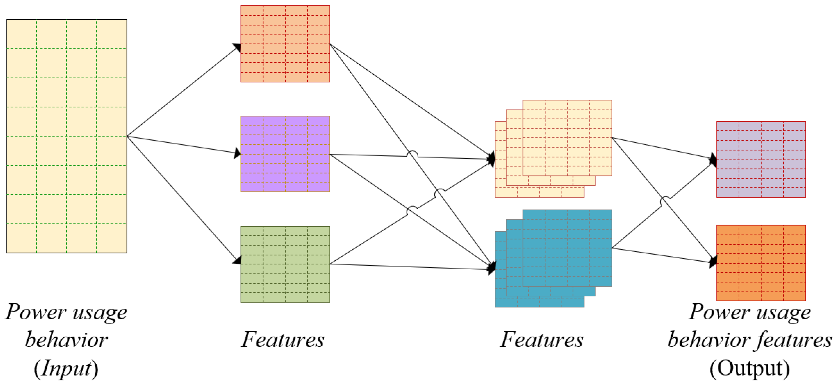
The convolutional neural network (CNN) module is used for feature extraction out of our model. The CNN model is usually stacked by the convolution layer and pooling layer. The convolution layer uses a set of convolution cores to extract abstract features, and the convolution operation is realized by the feature mapping of the input layer or intermediate layer through a convolution check. The structure of the CNN feature extraction module is illustrated in Figure 3.
For each calculation unit of the CNN module, we can use the following equation to obtain the feature value of power load data:
C i , j l = φ ( k n × 1 j × x i : i + n i + b i , j ) ,
where x i is the i-th channel of X, k n × 1 j represents ( i , j ) convolution kernel. Operation × represents convolution operation, and b i , j is offset.
Each convolution kernel processes the feature mapping of each channel, so the convolution layer can learn the representation in the time–frequency domain. Batch standardization and the ’Relu’ activation function can be used to process the output of each layer of convolution. Both can improve the convergence speed of CNN, and batch standardization can also improve the stability of CNN.
After the batch standardization and ’Relu’ activation function are added to the convolution layer, the local maximum pooling layer can be added to down-sample the eigenvalues to reduce the computational complexity, and the robustness of CNN in processing input variables is also improved. Therefore, we add a local maximum pooling layer after each convolution layer to optimize the performance of the CNN network.

4.3. Long Short-Term Memory Module

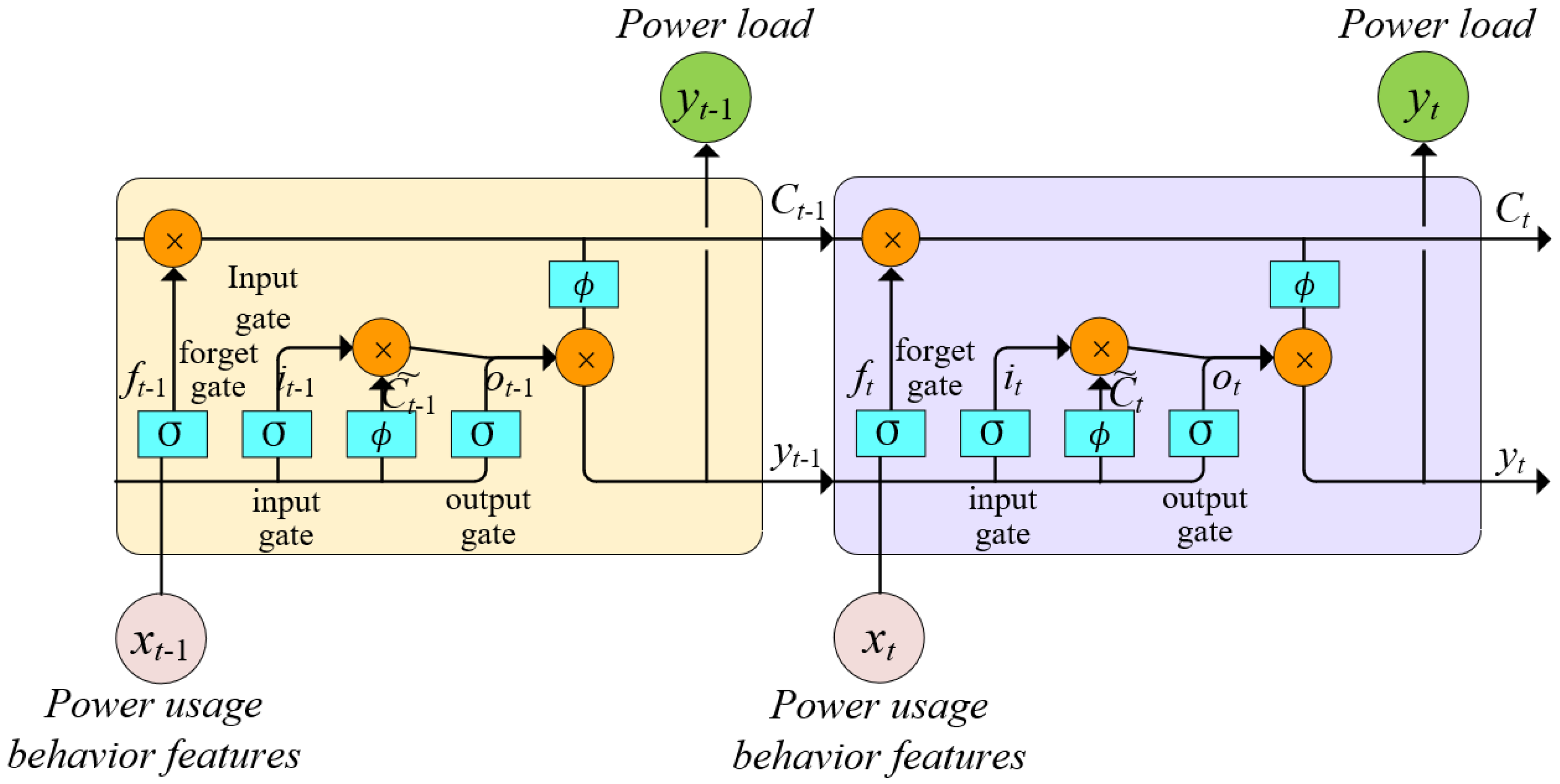
Long short-term memory (LSTM) neural networks have improved the neuron structure based on the cyclic neural network. LSTM uses the increased cell memory units to memorize and store the historical information of the distant past time. It also uses the gate structure to add, delete, and process information, ensuring that the cell information processing of the current iteration time has a strong time correlation with the distant past time information. In this way, the gradient disappearance phenomenon of RNN in long-time span sequence data processing can be solved. The detailed structure of LSTM is shown in Figure 4.
As shown in Figure 4, X t and Y t are cell input and output, respectively. LSTM has a memory unit C l s t to maintain cell state Y t and also has three fully connected nonlinear units. According to different weight matrices W and bias term b, and combined with the sigmoid function ϑ ( ) , a nonlinear conversion gate structure is achieved. The forgetting gate converts the current time input and the previous time output into 0 to 1 under the action of the sigmoid function. To control the amount of information transferred from the previous time to the current time, the forgetting gate F o r g e t t is used, for which the calculation equation is defined as:
F o r g e t t = ϑ ( W f o r g e t [ H t 1 , X t ] + b f o r g e t ) .
The input gate uses different weight matrices to control the information state of the input cell at the current time with the same mechanism, so as to prepare for the state update. For the input gate I n p u t t , the calculation equation is defined as:
I n p u t t = ϑ ( W i n p u t [ H t 1 , X t ] + b i n p u t ) .
The output gate obtains output based on the cell state, where the sigmoid layer performs quantitative control on the output part of the cell state. For the output gate O u t p u t t , the calculation equation is defined as:
O u t p u t t = ϑ ( W O u t p u t [ H t 1 , X t ] + b O u t p u t ) .
Finally, the output vector is classified by the ϱ ( ) activation function.
C l s t = ϱ ( W C l s [ H t 1 , X t ] + b C l s ) , Y t = O u t p u t t ϱ ( C l s t ) .
To effectively extract the power load features from time-series power load data in uncertain power systems, we further propose an improvement solution for the LSTM. We design a bi-directional CNN+ LSTM (CNN+BILSTM) model by changing the network structure of LSTM. Our proposed BILSTM combines the forward LSTM single model and the reverse LSTM single model. At the current iteration time, the reverse timing influence factors can be considered, which improves the model performance and data utilization efficiency. The forward and backward LSTM neuron layers embedded in the BILSTM network structure are connected with the sub-node layer, presenting two separate circular networks forward and backward. It combines the hidden layer states of the two LSTMs according to a specific combination method to provide more comprehensive information for the output layer. Then, it obtains the final prediction results of the power load data in the next period. BILSTM calculation includes forward and reverse processes. The forward calculation method is similar to the single LSTM model. The difference between the reverse calculation process and the forward calculation is that the state of the hidden layer at the next time is used in the reverse calculation.
In the improved CNN+BILSTM model, the forward calculation process is updated as:
F o r g e t t f = ϑ ( W F o r g e t f [ H t 1 , X t ] + b F o r g e t b ) , I n p u t t f = ϑ ( W I n p u t f [ H t 1 , X t ] + b I n p u t f ) , O u t p u t t f = ϑ ( W O u t p u t f [ H t 1 , X t ] + b O u t p u t f ) , C l s t f = ϱ ( W C l s f [ H t 1 , X t ] + b C l s f ) , Y t f = O u t p u t t f ϱ ( C l s t f ) .
In addition, the backward calculation process is defined as:
F o r g e t t b = ϑ ( W F o r g e t b [ H t 1 , X t ] + b F o r g e t b ) , I n p u t t b = ϑ ( W I n p u t b [ H t 1 , X t ] + b I n p u t b ) , O u t p u t t b = ϑ ( W O u t p u t b [ H t 1 , X t ] + b O u t p u t b ) , C l s t b = ϱ ( W C l s b [ H t 1 , X t ] + b C l s b ) , Y t b = O u t p u t t b ϱ ( C l s t b ) .

5. Experiments

In this section, we will carry out comparative experiments to verify the power load prediction capability of the proposed model in uncertain power systems. In Section 5.1, we will introduce the environmental setup, including the experimental platform, data sets, and evaluation indicators. The prediction accuracy and error of different algorithms will be discussed in Section 5.2. In Section 5.3, we further discuss the prediction accuracy and robustness of different algorithms in fluctuating power load data.

5.1. Experimental Setup

We used Python 3.9 to implement the proposed algorithm. All the selected algorithms use the code provided in the original paper and the original algorithm code encapsulated in the Sklearn library [36]. To reflect the fairness of the comparison experiment, each group of comparison experiments is conducted in the same hardware environment.
(1) Data sets.
In our comparative experiments, we use the historical power load data of Central China from 2015 to 2021 [37]. To reflect the uncertainty of the power system and the time fluctuation of power load data, our data sets include data from mountain areas, towns, residential areas, and industrial areas. Data sets from different areas have different power demands and data characteristics. The data from 2015 to 2020 are divided into training sets, and the data in 2021 are used as test sets.
The original tie-line power data have positives and negatives, which represent the power transmission direction. To speed up the algorithm convergence, the activation function of the CNN and LSTM modules uses the Relu function, and its output range is [ 0 , + ] . If the original data are directly input into the CNN-BILSTM model without processing, the reverse power data characteristics may be missed, which will reduce the prediction accuracy. Therefore, this article uses min–max to standardize the original data and restrict it into 0 and 1:
x = x x m i n x m a x x m i n
where x is the tie-line power data, and x is the normalized tie-line power data. Equation (15) is used to normalize the value of the power loads if power losses are not considered. This is because losses are a quadratic function of the power load. It does not depend on the direction of the flux but only on its value. By shifting the ’zero’ of the flux towards higher values, it is no longer possible to adequately account for losses.
(2) Evaluation Metrics
To evaluate the accuracy of the proposed CNN-BILSTM model, we use the MAPE and RMSE as our evaluation metrics, as defined as:
M A P E = 1 n t = 1 n y r ( t ) y p ( t ) y r ( t ) × 100 %
R M S E = 1 n t = 1 n ( y r ( t ) y p ( t ) ) 2
where y r ( t ) is the actual tie-line power, y p ( t ) is the predicted tie-line power, and n is the number of time points.

5.2. Experimental Results

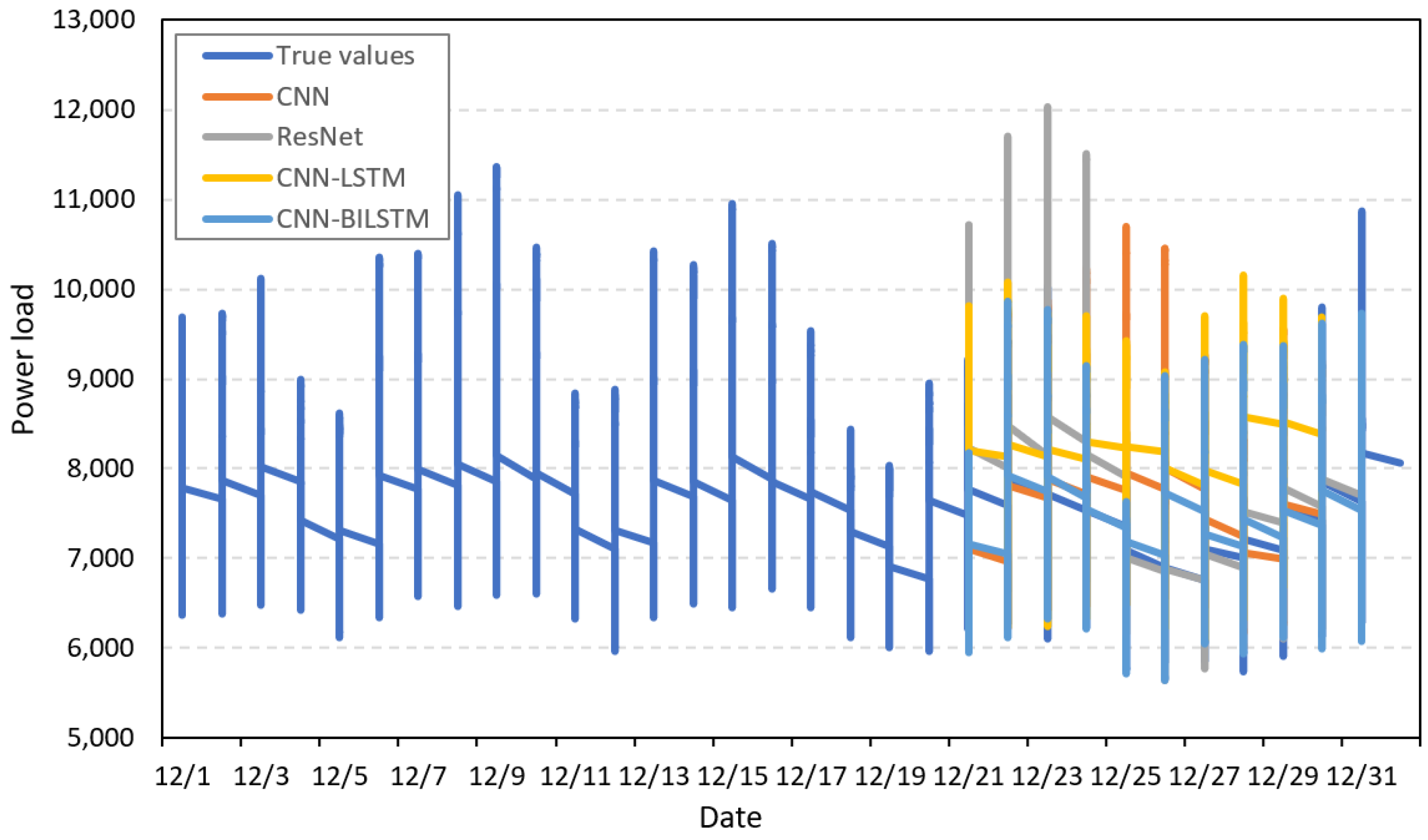
After the model parameters are ensured, the training set and test set data are entered into the model. Adam is used as the optimizer, the learning rate is 0.0025, the model is trained 100 times, and the power load on 30 July 2021 is predicted. To prove the superiority of the proposed CNN-BILSTM model, we compare the prediction results of tie-line power on 30 July 2021 with that of the ResNet and the LSTM model.
As seen in Figure 5, all three models can roughly predict the change in the trend of future tie-line power. Power load prediction in uncertain power systems is an intricate undertaking, involving the examination of the distribution and movement of electrical power within a network amid conditions of uncertainty. Given that the ResNet model is not inherently tailored for sequential data, it encounters challenges in addressing the temporal nature of power load prediction which heavily relies on time-dependent data. Consequently, the ResNet model demonstrates lower predictive accuracy in experimental results. Conversely, LSTM models appear as an appropriate choice due to their aptitude for capturing temporal dependencies and handling sequential data. Among these, our CNN-BILSTM model takes into consideration the numerical attributes inherent to power system power load prediction, yielding the most optimal predictive outcomes.
The loss function and error during the training process are shown in Figure 6 and Figure 7. The loss function is the MSE, and the error is represented by MAE.
From Figure 6 and Figure 7, we can see that among the three models, the CNN-BILSTM model has the fastest convergence speed and the smallest loss function and error. During training, ResNet might exhibit relatively higher training errors, especially if the data are sequential. ResNet’s deep architecture might help reduce training errors by enabling the model to learn complex relationships in uncertain power systems. However, if the task does not require such a deep architecture, there could be overfitting concerns. Our CNN-BILSTM model is well-suited for capturing temporal dependencies in sequential data. They are expected to yield lower training errors compared to CNN-LSTM and ResNet for tasks that involve time-dependent patterns, as they can effectively model these dependencies.

5.3. Ablation Experiments

We further conduct ablation experiments to analyze the performance of the model under different configurations and find out the optimal structure of the model to achieve the best performance. We use the CNN module, LSTM module, bidirectional LSTM module, and different loss functions respectively. Then, we record the model accuracy under each model structure and discuss the comparison results. The results of the ablation experiments are shown in Table 2.
We can see from Table 2 that the accuracy of power load prediction results varies with models of different structures. If only the CNN module is used, the prediction accuracy of the model is the lowest, only 64.25%. If the CNN module is used to extract the characteristics of power data first, and then LSTM is used to perform correlation analysis and prediction on the data in the time dimension, the accuracy of power load prediction is 68.18%. We improved the LSTM module and proposed the BILSTM module to improve the prediction accuracy of the model. We use three loss functions to realize reverse learning of the model, namely, Huber Loss, Quantitative Loss, and Cross Entropy Loss. Huber Loss is a loss function based on MSE and MAE losses, and the accuracy of its model is 89.27%. Quantile regression can fit different quantiles of the target value by giving different quantiles. Using quantile regression as the loss function, the accuracy of the model is 89.27%. In contrast, if we use Cross Entropy Loss as the loss function of the model, we can obtain the highest prediction accuracy of 92.87%.

5.4. Prediction Accuracy Comparison

Considering that the power load model in uncertain power systems has volatility, to research the forecasting stability of the algorithm proposed in this paper and other comparison algorithms, we further use more data forecasting algorithms for comparative experiments. Six kinds of real power load data with different fluctuation frequencies are used in the comparative experiments. The periods of the data sets are January, March, May, July, September, and November of 2021, respectively. We select the C4.5 classification prediction algorithm, Random Forest (RF) classification prediction algorithm, XGBoost algorithm, Convolutional Neural Network (CNN) algorithm, and Residual Network (ResNet) algorithm as the comparison algorithms. Each algorithm makes predictions in the six groups of data, records the prediction accuracy, and finally, takes their average value as the accuracy of the algorithm. For each algorithm, we separately count Accuracy, AUC, and F1 as the performance metrics. The experimental comparison results are shown in Table 3.
It can be seen from Table 3 that the prediction effect of the comparison algorithms on the volatile power load data sets is different. First of all, C4.5, RF, and XGBoost algorithms have limited feature extraction capabilities, so when the diversity of the power load data sets becomes greater, the prediction accuracy of these algorithms is not stable. For example, the average accuracy of the C4.5 algorithm on the six datasets is 68.36%, but the deviation is 8.14%. The average accuracy of the RF algorithm on the six datasets is 74.52%, but the deviation is 7.73%. In contrast, CNN and ResNet algorithms use convolution to extract data features, which can quickly extract effective data features and achieve higher accuracy. For example, the average AUC value of the CNN model on the six data sets is 88.74%, while the deviation is 3.26% and the average F1 value is 0.85. The average AUC value of the ResNet model on the six data sets is 90.26%, while the deviation is 3.92%, and the average F1 value is 0.89. Compared with other algorithms, the CNN-BILSTM algorithm proposed by us can not only extract the static features from the power load data at each time point but also extract the dynamic features with different time window lengths using the LSTM module. In this way, it can obtain robust prediction results on data sets with different volatility. Therefore, the CNN-BILSTM algorithm proposed in this paper has a high application value for the actual power load data processing.

6. Conclusions

This paper introduced an innovative Convolutional Neural Network–Bidirectional Long Short-term Memory (CNN-BILSTM) model to address the challenges posed by uncertain power conditions in power load prediction. By analyzing the inherent uncertainties of real-world power systems, we develop a data-driven power load model that forms the basis of the CNN-BILSTM architecture. The CNN-BILSTM model combines the advantages of CNN and BILSTM modules to achieve efficient feature extraction and capture the temporal dependencies in power load data. By integrating forward and backward LSTM modules, we enhance the model’s ability to predict power load timing, thereby improving overall performance and data utilization efficiency. Our comparative experiments confirm the effectiveness of the CNN-BILSTM model in predicting power load under uncertain conditions. The results demonstrate its potential for practical applications in industrial settings, providing reliable insights into grid operations and facilitating more accurate electricity demand forecasting.
In future research plans, we will explore multiple avenues to improve the accuracy and performance of the proposed CNN-BILSTM model. We will study the model’s performance under varying degrees of uncertainty and explore ways in which adaptive tuning of its parameters can provide valuable insights into its robustness and scalability. Additionally, exploring hybrid architectures that integrate CNN-BILSTM with other advanced deep learning techniques may lead to more accurate and efficient power load prediction models.

Author Contributions

Methodology, C.T.; Methodology, Z.T.; Investigation, F.W.; Resources, Y.Z. All authors have read and agreed to the published version of the manuscript.

Funding

This research is partially funded by the National Natural Science Foundation of China (Grant Nos. 62172146 and U23A20317).

Data Availability Statement

The original contributions presented in the study are included in the article, further inquiries can be directed to the corresponding author.

Conflicts of Interest

The authors declare no conflicts of interest. The funders had no role in the design of the study; in the collection, analyses, or interpretation of data; in the writing of the manuscript; or in the decision to publish the results.

References

  1. Dai, W.; Shi, B.; Li, T.; Goh, H.; Li, J. Power flow analysis considering solar road generation. Energy Rep. 2022, 8, 531–536. [Google Scholar] [CrossRef]
  2. Elgamal, M.; Korovkin, N.; Abdel Menaem, A.; Elmitwally, A. An algorithm for power flow analysis in isolated hybrid energy microgrid considering DG droop model and virtual impedance control loop. Sustain. Energy Grids Netw. 2022, 32, 100875. [Google Scholar] [CrossRef]
  3. Kumari, D.; Chattopadhyay, S.K.; Verma, A. Improvement of Power Flow Capability By Using An Alternative Power Flow Controller. IEEE Trans. Power Deliv. 2020, 35, 2353–2362. [Google Scholar] [CrossRef]
  4. Yue, Z.; Ding, Y.; Zhao, H.; Wang, Z. Ultra-high precise Stack-LSTM-CNN model of temperature-induced deflection of a cable-stayed bridge for detecting bridge state driven by monitoring data. Structures 2022, 45, 110–125. [Google Scholar] [CrossRef]
  5. Tang, C.Y.; Chen, P.T.; Jheng, J.H. Bidirectional Power Flow Control and Hybrid Charging Strategies for Three-Phase PV Power and Energy Storage Systems. IEEE Trans. Power Electron. 2021, 36, 12710–12720. [Google Scholar] [CrossRef]
  6. Lee, C.; An, J. LSTM-CNN model of drowsiness detection from multiple consciousness states acquired by EEG. Expert Syst. Appl. 2023, 213, 119032. [Google Scholar] [CrossRef]
  7. Lopez-Garcia, T.B.; Domínguez-Navarro, J.A. Power flow analysis via typed graph neural networks. Eng. Appl. Artif. Intell. 2023, 117, 105567. [Google Scholar] [CrossRef]
  8. Milano, F. Implicit Continuous Newton Method for Power Flow Analysis. IEEE Trans. Power Syst. 2019, 34, 3309–3311. [Google Scholar] [CrossRef]
  9. Khodaee, P.; Esfahanipour, A.; Mehtari Taheri, H. Forecasting turning points in stock price by applying a novel hybrid CNN-LSTM-ResNet model fed by 2D segmented images. Eng. Appl. Artif. Intell. 2022, 116, 105464. [Google Scholar] [CrossRef]
  10. Montoya, O.D.; Gil-González, W.; Garcés, A. A successive approximations method for power flow analysis in bipolar DC networks with asymmetric constant power terminals. Electr. Power Syst. Res. 2022, 211, 108264. [Google Scholar] [CrossRef]
  11. Portelinha, R.K.; Durce, C.C.; Tortelli, O.L.; Lourenço, E.M. Fast-decoupled power flow method for integrated analysis of transmission and distribution systems. Electr. Power Syst. Res. 2021, 196, 107215. [Google Scholar] [CrossRef]
  12. Chowdhury, B.H.; Taylor, C.W. Voltage stability analysis: VQ power flow simulation versus dynamic simulation. IEEE Trans. Power Syst. 2000, 15, 1354–1359. [Google Scholar] [CrossRef]
  13. Constante-Flores, G.E.; Illindala, M.S. Data-driven probabilistic power flow analysis for a distribution system with renewable energy sources using Monte Carlo simulation. IEEE Trans. Ind. Appl. 2018, 55, 174–181. [Google Scholar] [CrossRef]
  14. Fagundes, S.; Cardoso, F.; Stangler, E.; Neves, F.; Mezaroba, M. A detailed power flow analysis of the dual unified power quality conditioner (iUPQC) using power angle control (PAC). Electr. Power Syst. Res. 2021, 192, 106933. [Google Scholar] [CrossRef]
  15. Yoon, D.H.; Han, Y. Parallel power flow computation trends and applications: A review focusing on GPU. Energies 2020, 13, 2147. [Google Scholar] [CrossRef]
  16. Shekhar, A.; Soeiro, T.B.; Wu, Y.; Bauer, P. Optimal power flow control in parallel operating AC and DC distribution links. IEEE Trans. Ind. Electron. 2020, 68, 1695–1706. [Google Scholar] [CrossRef]
  17. Ahmadi, A.; Smith, M.C.; Collins, E.R.; Dargahi, V.; Jin, S. Fast Newton-Raphson power flow analysis based on sparse techniques and parallel processing. IEEE Trans. Power Syst. 2021, 37, 1695–1705. [Google Scholar] [CrossRef]
  18. Wu, X.W.; Zhu, L.F.; Wu, Z.M.; Ke, L.L. Vibrational power flow analysis of Timoshenko microbeams with a crack. Compos. Struct. 2022, 289, 115483. [Google Scholar] [CrossRef]
  19. Dalton, A.; Bekker, B.; Koivisto, M.J. Classified atmospheric states as operating scenarios in probabilistic power flow analysis for networks with high levels of wind power. Energy Rep. 2021, 7, 3775–3784. [Google Scholar] [CrossRef]
  20. Lu, K.D.; Zhou, L.; Wu, Z.G. Representation-learning-based CNN for intelligent attack localization and recovery of cyber-physical power systems. IEEE Trans. Neural Netw. Learn. Syst. 2024, 35, 6145–6155. [Google Scholar] [CrossRef]
  21. Aksan, F.; Li, Y.; Suresh, V.; Janik, P. CNN-LSTM vs. LSTM-CNN to Predict Power Flow Direction: A Case Study of the High-Voltage Subnet of Northeast Germany. Sensors 2023, 23, 901. [Google Scholar] [CrossRef]
  22. Li, Z.; Liu, H.; Zhao, J.; Bi, T.; Yang, Q. Fast power system event identification using enhanced LSTM network with renewable energy integration. IEEE Trans. Power Syst. 2021, 36, 4492–4502. [Google Scholar] [CrossRef]
  23. Yan, Z.; Xu, Y. Real-time optimal power flow: A lagrangian based deep reinforcement learning approach. IEEE Trans. Power Syst. 2020, 35, 3270–3273. [Google Scholar] [CrossRef]
  24. Sayed, A.R.; Wang, C.; Anis, H.I.; Bi, T. Feasibility constrained online calculation for real-time optimal power flow: A convex constrained deep reinforcement learning approach. IEEE Trans. Power Syst. 2022, 38, 5215–5227. [Google Scholar] [CrossRef]
  25. Putri, S.M.; Maizana, D.; Bahri, Z. Analysis of smart grid power flow system with Gauss-Seidel method. In IOP Conference Series: Earth and Environmental Science; IOP Publishing: Bristol, UK, 2021; Volume 753, p. 012005. [Google Scholar]
  26. Chamim, A.N.N.; Putra, K.T.; Al Farisi, M.F. Power Flow Analysis of Electrical Network Systems Using Gauss-Seidel Method and Python. Emerg. Inf. Sci. Technol. 2023, 4, 28–36. [Google Scholar]
  27. Chen, Y.; Zhao, Y.; Ma, J. Fast decoupled multi-energy flow calculation for integrated energy system. J. Mod. Power Syst. Clean Energy 2020, 8, 951–960. [Google Scholar] [CrossRef]
  28. Coutinho de Oliveira, C.; Bonini Neto, A.; Alves, D.A.; Minussi, C.R.; Castro, C.A. Alternative Current Injection Newton and Fast Decoupled Power Flow. Energies 2023, 16, 2548. [Google Scholar] [CrossRef]
  29. Tang, K.; Dong, S.; Song, Y. Successive-intersection-approximation-based power flow method for integrated transmission and distribution networks. IEEE Trans. Power Syst. 2020, 35, 4836–4846. [Google Scholar] [CrossRef]
  30. Liu, Y.; Li, Z.; Fan, M. A Newton–Raphson-based sequential power flow algorithm for hybrid AC/DC microgrids. IEEE Trans. Ind. Appl. 2021, 58, 843–854. [Google Scholar] [CrossRef]
  31. Sun, W.; Zamani, M.; Zhang, H.T.; Li, Y. Probabilistic optimal power flow with correlated wind power uncertainty via Markov chain quasi-Monte-Carlo sampling. IEEE Trans. Ind. Inform. 2019, 15, 6058–6069. [Google Scholar] [CrossRef]
  32. Palahalli, H.; Maffezzoni, P.; Gruosso, G. Modeling photovoltaic generation uncertainties for monte carlo method based probabilistic load flow analysis of distribution network. In Proceedings of the 2020 55th International Universities Power Engineering Conference (UPEC), Online, 1–4 September 2020; pp. 1–6. [Google Scholar]
  33. Jabari, F.; Shamizadeh, M.; Mohammadi-Ivatloo, B. Probabilistic power flow analysis of distribution systems using Monte Carlo simulations. In Optimization of Power System Problems: Methods, Algorithms and MATLAB Codes; Springer: Berlin/Heidelberg, Germany, 2020; pp. 215–232. [Google Scholar]
  34. Ni, F.; Nguyen, P.H.; Cobben, J.F. Basis-adaptive sparse polynomial chaos expansion for probabilistic power flow. IEEE Trans. Power Syst. 2016, 32, 694–704. [Google Scholar] [CrossRef]
  35. Mühlpfordt, T.; Roald, L.; Hagenmeyer, V.; Faulwasser, T.; Misra, S. Chance-constrained AC optimal power flow: A polynomial chaos approach. IEEE Trans. Power Syst. 2019, 34, 4806–4816. [Google Scholar] [CrossRef]
  36. Scikit Learn. Sikit-Learn: Machine Learning in Python. 2024. Available online: https://scikit-learn.org (accessed on 1 January 2024).
  37. CSDN. Power System Load Forecasting Data Set. 2024. Available online: https://download.csdn.net/download/qq_25888559/28453108 (accessed on 1 January 2024).
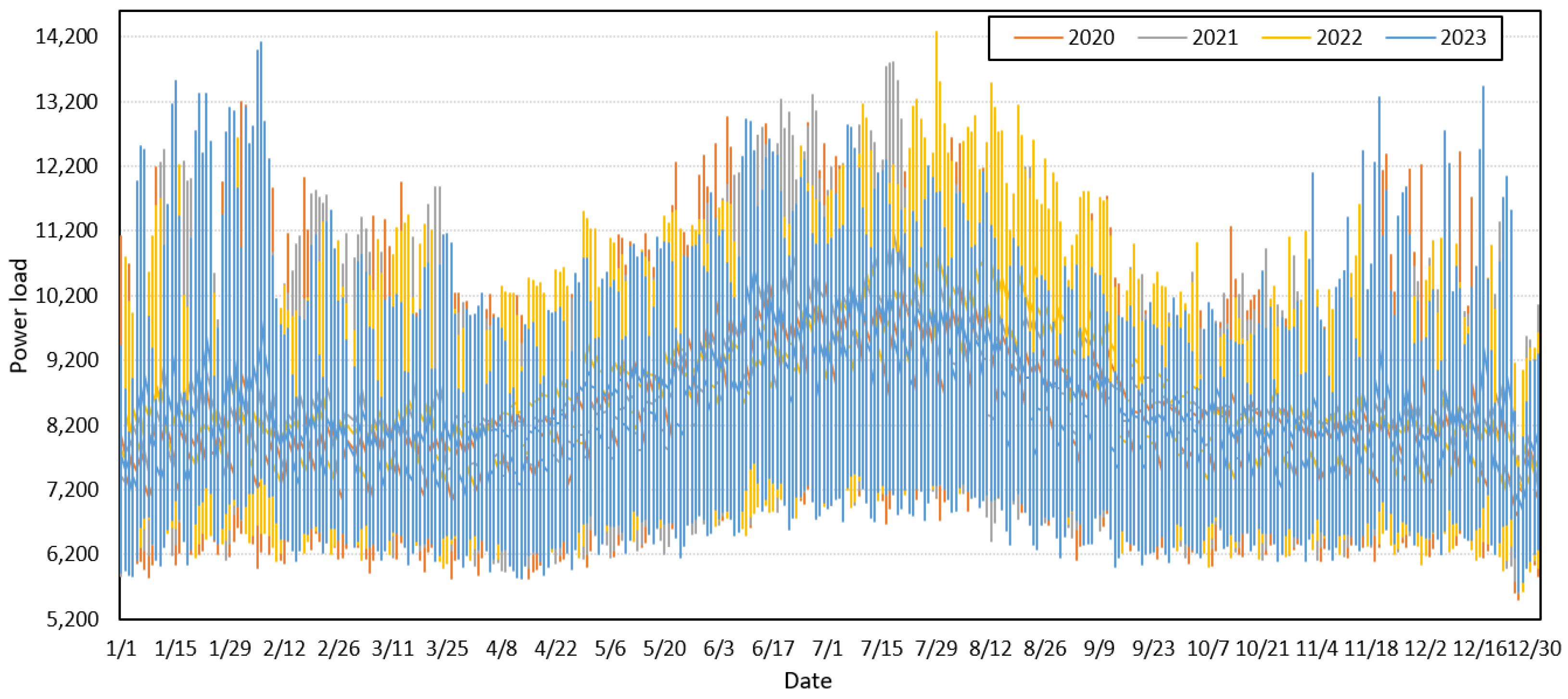
Figure 1. Distribution of power load of multiple power plants in China between 2020 and 2023.
Energies 17 02312 g001
Figure 2. Overall architecture of the improved CNN-BILSTM model for power load prediction.
Energies 17 02312 g002
Figure 3. Structure of the convolutional neural network (CNN) module.
Energies 17 02312 g003
Figure 4. Structure of the long short-term memory (LSTM) neural network model.
Energies 17 02312 g004
Figure 5. Comparison of prediction accuracy.
Energies 17 02312 g005
Figure 6. Comparison of loss function.
Energies 17 02312 g006
Figure 7. Comparison of training errors.
Energies 17 02312 g007
Table 1. Structure and parameters of the proposed CNN-BILSTM model.
No.ModulesLayersParametersVaules
1CNNConv1D-1kernel size3
2CNNConv1D-1filters100
3CNNConv1D-2kernel size3
4CNNConv1D-2filters64
5CNNMaxPooling1D-1pool size2
6CNNMaxPooling1D-2pool size2
7LSTMLSTM-1units32
8LSTMLSTM-2units16
9DenseDense-1units128
10DenseDense-2units32
11DenseDense-3units2
Table 2. Results of ablation experiments of our CNN-BILSTM model.
MethodsAccuracyAUCF1 Score
CNN module64.25%72.24%0.68
CNN + LSTM modules68.18%75.73%0.71
CNN + BILSTM + Huber Loss89.27%90.51%0.85
CNN + BILSTM + Quantile Loss92.48%91.34%0.89
CNN + BILSTM + Cross Entropy Loss92.87%93.01%0.90
Table 3. Prediction accuracy comparison between different algorithms.
MethodsAccuracyAUCF1 Score
C4.568.36% ± 8.14%75.42% ± 9.53%0.70
RF74.52% ± 7.73%80.16% ± 6.98%0.72
XGBoost76.19% ± 7.49%83.58% ± 7.75%0.79
CNN78.36% ± 3.44%88.74% ± 3.26%0.85
ResNet86.83% ± 3.62%90.26% ± 3.92%0.89
CNN-BILSTM92.15% ± 2.14%94.87% ± 2.13%0.95
Disclaimer/Publisher’s Note: The statements, opinions and data contained in all publications are solely those of the individual author(s) and contributor(s) and not of MDPI and/or the editor(s). MDPI and/or the editor(s) disclaim responsibility for any injury to people or property resulting from any ideas, methods, instructions or products referred to in the content.