Article

Accuracy of Simscape Solar Cell Block for Modeling a Partially Shaded Photovoltaic Module

Department of Electronics and Computing, Faculty of Electrical Engineering, Mechanical Engineering and Naval Architecture, University of Split, 21000 Split, Croatia
*
Author to whom correspondence should be addressed.
Energies 2024, 17(10), 2276; https://doi.org/10.3390/en17102276
Submission received: 14 April 2024 / Revised: 30 April 2024 / Accepted: 7 May 2024 / Published: 9 May 2024
(This article belongs to the Special Issue Advances in Solar Systems and Energy Efficiency)

Abstract

:
With half-cut photovoltaic (PV) modules being the dominant technology on the market, there is an increasing necessity for accurate modeling of this module type. Circuit simulators such as Simulink are widely used to study different topics regarding photovoltaics, often employing a solar cell block available from the Simcape library. The purpose of this work is to validate this model against measurements for a partially shaded half-cut PV module. Diverse shading scenarios are created by varying the number of shaded substrings, the number of shaded solar cells in the substring, and the shading level. For every shading scenario, the PV module’s I-V curve is measured, along with in-plane irradiance, air temperature, and module temperature. A comprehensive evaluation of simulation accuracy is presented. The results confirm a high accuracy of the model with mean nRMSE values of 2.2% for I-V curves and 2.8% when P-V curves are considered. It is found that the simulation errors tend to increase when increasing the number of shaded substrings. At the same time, no obvious dependency of simulation accuracy on the shading level or the number of shaded solar cells in the substring is found.

1. Introduction

Shading has been long recognized as one of the most serious loss mechanisms in photovoltaics. It causes uneven irradiance of the photovoltaic (PV) module and induces mismatch losses because the electrical output of the shaded solar cell is significantly reduced. However, in many practical applications, shading is unavoidable. This is especially true in urban areas, where neighboring buildings, trees, or other objects during some part of the day often cast shade on the rooftop photovoltaic system. The magnitude of the losses depends on the shaded area and the intra- and inter-module wiring topology. A single crystalline–silicon solar cell typically has a voltage of 0.5–0.6 V. Practical applications generally require higher voltages, so inside the photovoltaic module, solar cells are traditionally connected in series. Similarly, a series connection of photovoltaic modules in the photovoltaic array is often used to avoid high currents that increase cabling losses. Unfortunately, a series connection is the most prone to shading losses. Shading a solar cell significantly reduces its current, while the decrease in output voltage becomes much lower. However, the reduced current from the shaded solar cell impacts the whole string of cells connected in series, and this detrimental effect is further transferred to the PV array. Theoretically, a complete shading of a single cell in a single PV module would reduce the current from the PV module to zero, and consequently, the output of the complete string of PV modules would be reduced to zero. A conventional method of mitigating this effect is to use bypass diodes, typically connected in parallel to the string of series-connected solar cells. Usually, three bypass diodes per PV module are used. That means the PV module is split into three parts, usually termed submodules, and each of them has a corresponding bypass diode. When the shadow appears on some part of the submodule, the current is passed through its bypass diode, meaning the whole submodule is excluded from the total PV module output. A shadow on one submodule thus causes the reduction in approximately one-third in the PV module output power.
PV models are pivotal for PV system planning and analysis. They are used, among other issues, for studying PV system output characteristics under partial shading and the development of new maximum power point tracking (MPPT) algorithms. As shading patterns across the PV array can be complex, accurate modeling of PV module output characteristics under partial shading is crucial for a reliable assessment of PV system performance and electricity production.
Studies of the shading effect on PV performance differ in terms of resolution. The coarsest view considers shading on the PV module level only, i.e., it is assumed that every module is uniformly illuminated or shadowed. This approach can be adequate for PV systems comprising many PV modules, such as in [1], where the authors analyzed the shading effect on the output of a PV array with 1000 PV modules. Yet, some authors have used the same approach even for smaller PV arrays, having as little as 21 PV modules [2] or 6 PV modules [3]. However, it was shown in [4] that module-level modeling results in an inaccurate estimation of the total system power and maximum power point voltage. Modeling accuracy can be improved if the shading is considered at the substring level, where the substring refers to a string of series-connected PV cells protected by a bypass diode. This was used in [5], where partial shading of a single PV module and mismatch losses of a string of 18 PV modules connected in series were considered, increasing the shaded area in steps of one-third of the total PV module area. The best resolution in modeling the partial shading is achieved if the shading is observed at the cell level. The studies performed on the single solar cell have confirmed that a partially shaded solar cell behaves as if it is uniformly illuminated by the reduced irradiance, with the reduction proportional to the shaded area [6]. Hence, when modeling the PV system under partial shading, an equivalent circuit model of a solar cell can be used as the main building block.
Commonly, the single diode model of a solar cell is used, because it is simple and still provides reasonable accuracy. Another diode is added to improve the model accuracy at low voltages when the recombination in the junction region becomes significant. More details about solar cell models can be found elsewhere [7,8,9]. If the number of series- and parallel-connected solar cells in the PV module is known, the equation describing the solar cell equivalent circuit is easily scaled to obtain the current–voltage dependence of the PV module. Unfortunately, the equation is implicit and the main challenge is to determine the model parameters. Many different numerical and analytical methods to obtain the model parameters have been proposed, and several review papers on the topic have been published [10,11,12,13]. It should be noted that a comprehensive review of PV system models under partial shading showed that many published studies lack experimental validation [14]. Regardless of the choice of a numerical or analytical approach, the extraction of the model parameters requires a high level of expertise and mathematical knowledge.
Modeling the effects of partial shading using MATLAB/Simulink is convenient and frequently used because the solar cell model is available as a standard simulation block in the Simscape library. This allows for the shading analysis to be conducted at the cell level. The block has two output ports belonging to positive and negative terminals, and one input port for irradiance. Input thermal port can be optionally enabled. Solar cell block as available in the Simscape library is built as a two-diode equivalent circuit model of the solar cell [15], but the user can choose to reduce the complexity by using a single-diode model or neglect the leakage current losses. The Simscape solar cell block has predefined parameters for three different parameterizations, and these parameters should be confirmed by measured data to ensure the model’s accuracy. Due to the popularity and widespread use of MATLAB/Simulink in the scientific community, many different topics have been studied using simulations that are based on the Simscape solar cell block [16,17,18,19,20]. It is especially suitable for simulating circuits where photovoltaic modules are connected to other circuit elements, such as DC/DC converters, batteries, etc.
However, to the best of the authors’ knowledge, a rigorous estimation of the accuracy of the Simscape solar cell block and its suitability for simulating PV systems under partial shading has not been published elsewhere. This is especially true when considering the scarcity of studies on Simscape block accuracy for modeling partially shaded half-cut PV modules. The SPICE-based simulations demonstrated that half-cut PV modules are superior to full-cell modules under partial shading conditions [21,22]. Hotspot temperature simulations using the single-diode solar cell model and Bishop’s reverse breakdown model implemented in MATLAB further showed that half-cut PV modules also exhibit lower local heating [23]. Although the half-cut technology accounted for more than 90% of all PV modules in 2022 [24] and is currently dominant on the market, a literature survey reveals only a limited number of experimental studies of partial shading for half-cut PV technology. In [25], the authors studied the influence of shading on three different configurations of half-cut modules. Two distinct scenarios were considered: in the first case, only a certain area of the single solar cell was shaded, and in the second the shaded area was subsequently increased along the longer and shorter PV module side. No comparison of measurement and simulations was given, and only one shading level was considered. The output characteristic of a half-cell PV module under partial shading has been simulated using MATLAB/Simulink [26]. However, only four shading scenarios were considered, varying only the size of the shaded area. A semi-transparent polyethylene film was used for shading in experiments, reducing the irradiance of the shaded solar cells approximately by half. A comparison of simulation and measurement results was given for the case of unshaded PVmodule alone and only in terms of relative error for the typical parameters (short-circuit current, open-circuit voltage, efficiency, fill factor).
The main contributions of this study can be summarized as follows:
  • Thorough validation of the Simscape solar cell model in partially shaded conditions, considering a wide range of shading scenarios;
  • Improved methodology for comprehensive model evaluation, based on comparison along entire I-V and P-V curves;
  • Experimental validation using a half-cut PV module;
  • Initial estimation of how different shading parameters influence the model’s error.

2. Materials and Methods

Initially, different shading scenarios for the experiment are designed. Only cell-level shading is considered because partial shading of a single solar cell has the same effect as homogeneous illumination of the total solar cell area but with reduced irradiance [27,28]. Different shading scenarios are created by using three different shading levels and by varying the number of the shaded solar cells and the number and position of substrings where the shade occurs. The output I-V curves of the half-cut PV module are measured for every shading scenario. Then, each case is simulated in MATLAB/Simulink, using the model of the PV module based on the built-in Simscape solar cell block. It should be noted that the intent of this work is not to propose a new model but to check the existing one using it with as little adjustment as possible. The accuracy of the model is estimated by comparing the difference between the simulated and measured I-V and P-V curves. In many existing studies, the evaluation is focused only on three typical points on the I-V curve, so usually only the relative error for short-circuit current, open-circuit voltage, and maximum power current and voltage is given (see, e.g., [26,29,30]). In this paper, the differences between simulation and measurement along the entire I-V and P-V curves are considered when estimating the accuracy of the simulation for a particular shading scenario.

2.1. Experimental Details

Three polyethylene sheets with different transmittances were used to create different shading levels, denoted as T1–T3, with T1 having the highest transmittance. The spectrum of the shading sheets was measured using an EKO MS-711 spectroradiometer from EKO Instruments, Co., Ltd., Tokyo, Japan [31], covering a 300–1100 nm region. The measured spectra are shown in Figure 1 along with a spectrum of the “regular” shade. Then, by comparison with the spectrum measured without shading the spectroradiometer, the spectrally weighted transmittance of each sheet was calculated. The resulting transmittance values for sheets T1–T3 were 61%, 36%, and 14%, respectively. These values represent the percentage of solar radiation that passes through a sheet in the considered wavelength region. Transmittances T1 and T2 were practically independent of the wavelength, as is the case for the regular shade, while transmittance T3 increased nearly linearly with the wavelength. However, near the edge of the recorded spectrum, the sensitivity of the silicon solar cells was significantly reduced [32], so this effect can be neglected without affecting the results of the study. Therefore, sheet T3 was used to represent a “regular” shade. Despite some differences in the spectrum, this is a much more realistic scenario than using completely non-transparent material, an approach commonly found in the literature.
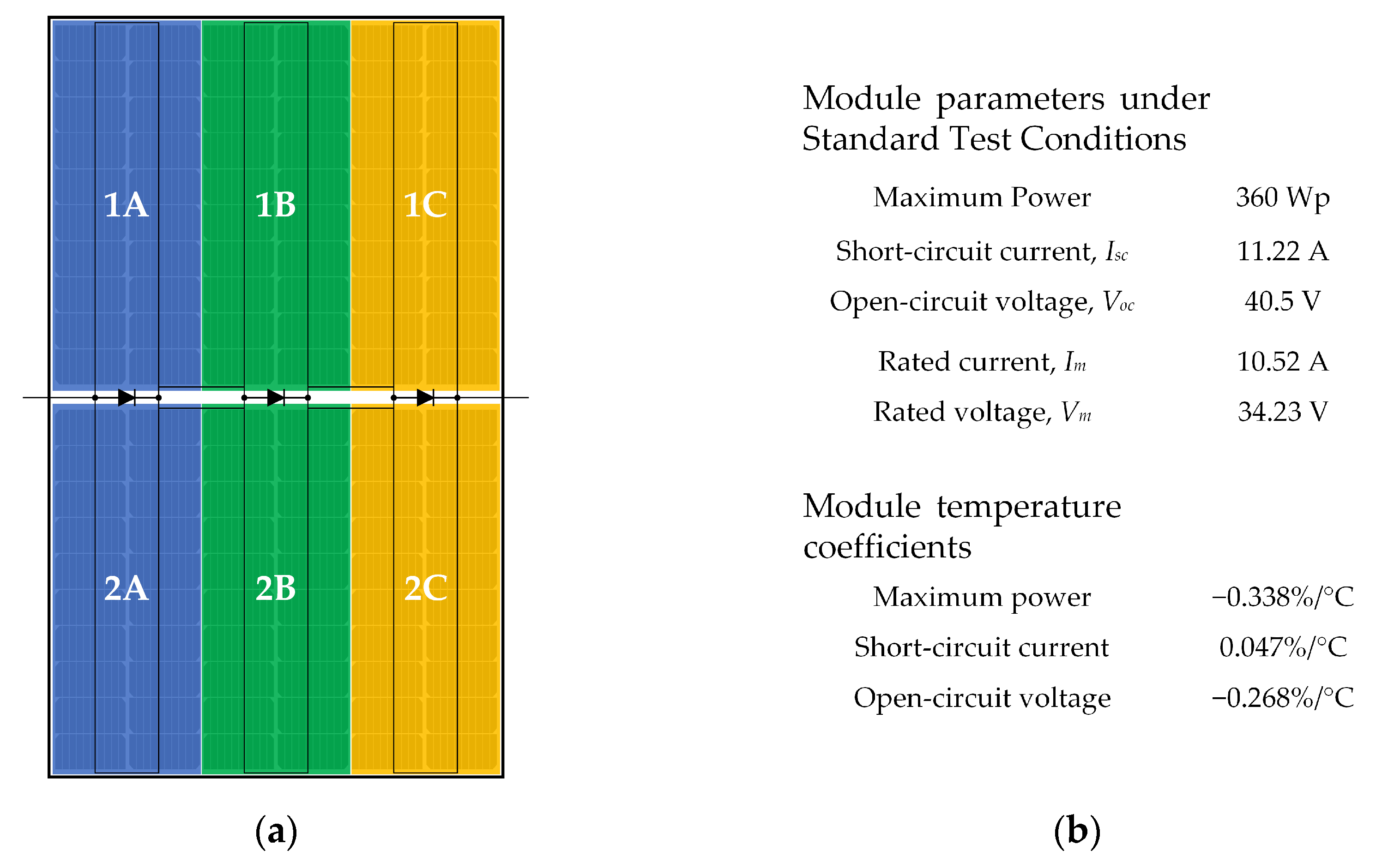
A half-cut PV module SV120-360 E BC HC9B [33] from Croatian manufacturer Solvis d.o.o., Varaždin, Croatia, was used for the experiment. This module consists of 120 monocrystalline solar cells, each with a size of 166 mm × 83 mm. The module is split into two halves connected in parallel, with each half comprising 3 substrings of 20 solar cells in series. Just like in the case of full-cell PV modules, there are three bypass diodes, every diode connected in parallel to the series string of 20 solar cells. In the case of half-cut PV modules, individual bypass diode is therefore shared by the two substrings from the opposing halves of the PV module. Overall, the half-cut PV module can be considered to comprise six substrings of 20 solar cells in series. The internal structure of the module is illustrated in Figure 2a. For easier understanding, each 20-cell substring is labeled using numbers 1 and 2 to designate the upper (1) and lower (2) half of the module, and letters A, B, and C designate the bypass diode that is connected to the considered substring. Additionally, the main parameters of the PV module are given in Figure 2b.
The tested PV module was fixed on the mounting frame with a 23° tilt facing due south and placed on the roof of the Faculty of Electrical Engineering, Mechanical Engineering, and Naval Architecture in Split, Croatia (43.5115° N, 16.4696° E).
Measurements were taken in July 2023 during the hours around solar noon on clear sky days to minimize the losses caused by the high incidence angle. A portable I-V Checker EKO MP-11 from EKO Instruments, Co., Ltd., Tokyo, Japan [34] was used to record I-V curves. The instrument records 400 data points of the I-V curve with a voltage resolution of 10 mV and a current resolution of 10 mA, taking between 4 and 640 ms to complete the sweep. Both voltage and current measurement accuracy were within ±1.0% of full scale over the voltage and current range. Simultaneously, plane-of-array (POA) irradiance was measured by the instrument’s sensor unit. The integrated pyranometer can measure irradiance up to 1500 W/m2, with an accuracy within 1.5% of full scale. Also, the temperature of the PV module’s rear surface and air temperature were measured using two T-type thermocouples supplied with the sensor unit. A sequence of measurements was performed using different shading sheets for each shading scenario. The typical time between subsequent measurements was around 30 s, so the irradiance was practically unchanged. Shading was achieved by closely covering the part of the PV module with the selected shading sheet.
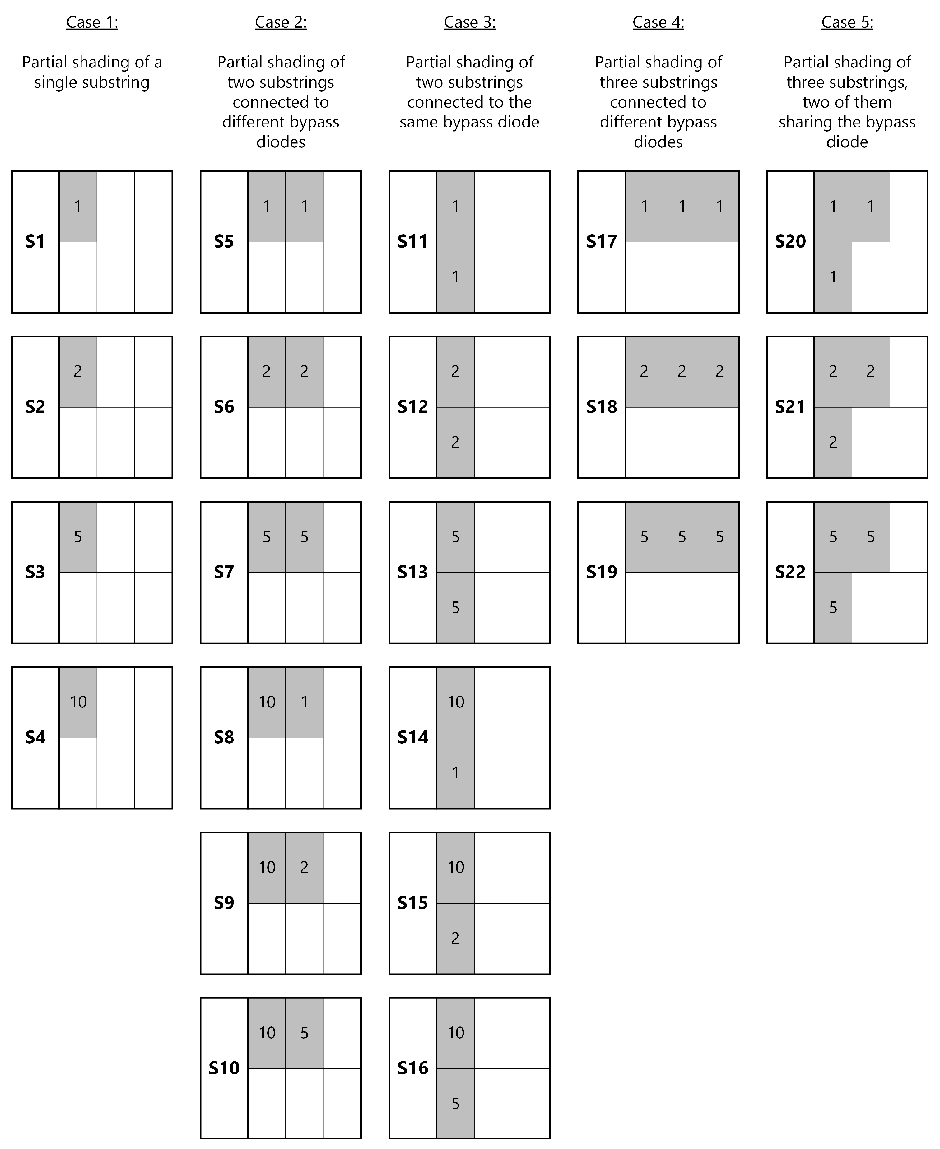
Different shading patterns are created by varying the number of the shaded substrings, the number of shaded cells in a particular string, and the shading level is determined using sheets with different transmittance. Shading scenarios are grouped into five distinctive cases based on the number of shaded substrings and their position within the module, as illustrated in Figure 3. As can be seen in the figure, considered scenarios include from one to three partially shaded substrings. This is because the biggest changes in I-V and P-V curves come from the activation of bypass diodes. By considering up to three shaded substrings, we were able to design scenarios in which one (Cases 1 and 3), two (Cases 2 and 5), or all three bypass diodes were activated (Case 4). With three different shading levels used in every scenario, 66 unique conditions in total were analyzed.

2.2. Modeling and Simulation

The model of the half-cut PV module under study is built in Simulink (MATLAB R2023a with Simulink v. 10.7 was used) by connecting 120 Simscape solar cell blocks and three bypass diodes in accordance with the module structure illustrated in Figure 2a. As described, the module consists of six substrings, each having 20 solar cells in series. Solar cell parameters in Simulink can be defined in three ways:
(a)
5 parameters using short-circuit current (Isc) and open-circuit voltage (Voc);
(b)
5 parameters using parameters of an equivalent circuit model;
(c)
8 parameters using parameters of a double-diode equivalent circuit model.
In this work, the first option is selected because Isc and Voc are usually available from the PV module datasheet given by the manufacturer, which makes it the simplest option to employ. Additionally, the temperature coefficient for Isc from the datasheet is entered into the model. It should be noted that the selected model neglects the solar cell’s shunt resistance.
According to Simscape library documentation [35], for the chosen 5-parameter solar cell model, the output current, I, is given by
I = I p h I s exp V + I R s m V T 1 ,
where Iph is the photogenerated current, Is is the diode saturation current, V is the output voltage, Rs is the series resistance, m is the diode ideality factor, and VT is the thermal voltage.
Initially, the unknown solar cell parameters (the diode ideality factor and solar cell series resistance) are adjusted by fitting the model to measured I-V curves when the PV module is unshaded. This is regarded as a referent scenario, S0. MATLAB’s Curve Fitting Toolbox is used to obtain the missing parameters.
Afterward, the solar cell parameters are considered to be constant, and only measured POA irradiance and temperature of the PV module’s rear surface are entered into the model, assuming the temperature of all solar cells in the module is equal. Under partial shading, this assumption might not be correct, but the effect of the temperature gradient is out of the scope of this study and is believed not to have a significant impact on the conclusions.

2.3. Metrics for Estimation of the Model Accuracy

The accuracy of the simulation model for a particular shading scenario is estimated using a two-level assessment:
Partial assessment concentrating on three typical points on the I-V curve: short-circuit current, open-circuit voltage, and maximum power point. The relative error is calculated using the following expression:
X r e l = X s X m X m 100 % ,
where Xrel stands for relative error, Xs is the simulation value, and Xm is the measured value of particular quantity X. It should be noted that in cases with more than one inflection point on the P-V curve, only the global maximum power point is considered. Besides the values of maximum power (Pm), corresponding current (Im) and voltage (Vm) values are also included in the evaluation.
Thorough assessment taking into account the differences between simulation and measurement along entire I-V and P-V curves. In fact, due to the reduced accuracy of the used I-V curve tracer for currents below 0.3 A, this part of the curve is excluded from the analysis. The agreement between the simulated and measured curves is estimated using common parameters for statistical metrics: mean bias error (MBE), mean absolute error (MAE), and root mean square error (RMSE). These parameters are normalized by the measured value of short-circuit current when analyzing the I-V curve, and by the measured value of global maximum power for the P-V curve. The main reason for normalization is reduction in the impact of varying irradiance and temperature throughout the measurements. The short-circuit current is directly proportional to irradiance, so at higher irradiance levels the output current and power increase. As a result, at higher irradiance, the larger absolute value of the specific metric parameter might at the same time have a smaller relative value. Hence, normalization by the short-circuit current is used to account for varying irradiance and temperature, and this is widely accepted in the scientific community [36,37,38,39]. Similarly, when P-V curves are considered, the maximum power is selected for normalization to facilitate the comparison of the results obtained under different irradiance values and temperatures, as well as different shading scenarios. Hence, the expressions used are given as
nMBE = 1 N i = 1 N X s X m X max ,
nMAE = 1 N i = 1 N X s X m X max ,
nRMSE = 1 N i = 1 N X s X m 2 X max
where N is the number of points along the I-V and P-V curves, Xmax stands for Isc in the case of the I-V curve and Pm for the P-V curve.
For a reliable accuracy assessment, the number of points should be sufficiently large. Since the deviation between measured and simulated curves varies along the voltage axis, taking too few points could cause misleading results. So, in all scenarios, between 365 and 380 points are taken with the linear voltage resolution of 0.1 V. This ensures that all voltage regions, including the critical ones where the highest discrepancy occurs, are well covered.

3. Results

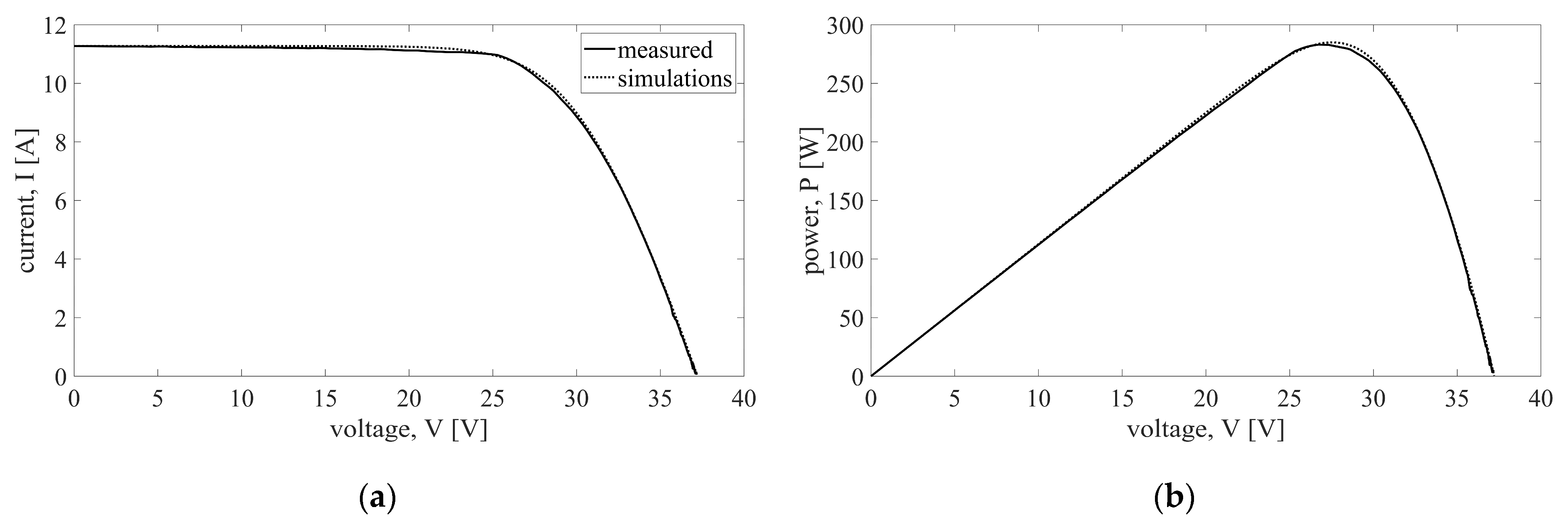
A referent scenario S0 for the case of an unshaded PV module is used to fit the model to the measurements. Two missing model parameters, diode ideality factor n and series resistance Rs are found in this way. The obtained values are n = 1.2 for the diode ideality factor and Rs = 15 mΩ for series resistance. These values, together with the temperature coefficient, are kept constant throughout the rest of the simulations. The difference between simulations and measurements for the referent scenario S0 is shown in Figure 4. The relative errors are 0.7% for Pm and 0.8% for Voc, with practically equal Isc in simulations and measurements. There is, however, a slight disagreement in the values of current, Im, and voltage, Vm, in the maximum power point. The relative error for maximum power current is −2.4%, and the corresponding voltage error is 3.1%. If the complete I-V and P-V curves are analyzed, the obtained nRMSEs are 0.67% for the I-V curve and 0.64% for the P-V curve. It is interesting to note that nMBE values are positive for both curve types, indicating the slight tendency of the simulations to overestimate the current and power for a particular voltage value. Nevertheless, the obtained errors are very low, so it can be considered that for the referent unshaded PV module scenario the model fits measurement with high accuracy.
When shaded scenarios are taken into account, the agreement between the simulations and measurements is slightly lower. The results of all 22 shading scenarios depicted in Figure 3 in combination with three transmittance levels, giving out 66 unique conditions in total, are summarized in Table 1. For all parameters used to evaluate the simulation accuracy and defined in Section 2.3, the mean and maximum values are calculated. It should be noted that for parameters that can be negative (relative errors and nMBEs), the mean for each parameter is calculated using absolute values to avoid the error from partial cancellation of positive and negative values. The highest relative error is obtained for the value and position of the maximum power, but the mean of these values remains below 3.5%, indicating the existence of an outlier. This outlier is further commented on in a separate analysis of each case. The highest relative error of the maximum power is 5.1%, but on average this value is less than 2.2%. Very good agreement of simulations to measurements is also confirmed by low errors when the complete I-V and P-V curves are studied, with mean values for all error parameters of ≤2.8%.

3.1. Partial Shading of a Single Substring (Case 1)

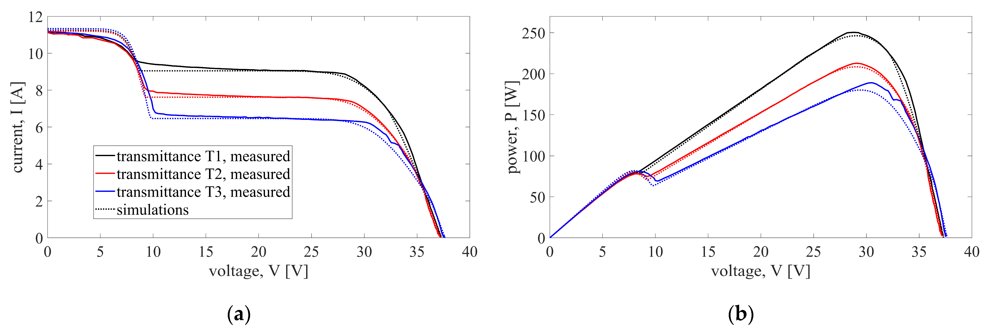
It is well known that the shading of a single solar cell can activate the bypass diode, circumventing the current flow of the whole series substring. Despite that, partial shading of a single substring included four scenarios with 1, 2, 5, and 10 shaded solar cells from the same substring. The experimental results confirmed that increasing the number of shaded cells in the substring makes a marginal impact on the output characteristics. Therefore, the comparison between simulations and measurements is shown in Figure 5 only for scenario S1 with only one shaded solar cell. The characteristics are given for all three shading sheets with transmittances T1–T3. For all three shading levels, two major disagreements can be observed. First, activation of the bypass diode causes abrupt changes in the curves obtained by simulations, while the measurements show that the actual changes are somewhat gradual. This can be seen for voltages around 20 V. Another noticeable difference occurs for voltages above 30 V, where the simulated curves start decreasing before the measured ones. As a result, the simulations underestimate the maximum power, but this underestimation is rather small with a relative error of −2.1% for the sheet with the highest transmittance T1, −3.3% for the sheet with transmittance T2, and −2% for the sheet with transmittance T3. In all other scenarios belonging to this case (S2–S4), the results are even better, with smaller errors. The error metrics show a high level of the model’s accuracy when the agreement along the curves is analyzed. The highest value of nRMSE is 2.1% for the I-V curve (obtained for shading level T1, Scenario 4), while for the P-V curve, the highest nRMSE is 3.5% (shading level T3, Scenario 4). All other errors are typically less than ±2% and are given in Table 2.

3.2. Partial Shading of Two Substrings (Cases 2 and 3)

Two distinctive cases can be recognized when considering the shading of two substrings, marked as Case 2 and Case 3 in Figure 3.
The first of the cases occurs when two shaded substrings are connected to different bypass diodes. In such a situation, there are 12 possible pairs of shaded substrings, but the actual combination does not affect the PV module output. Of course, this assumption is valid provided that all solar cells in the module are identical. As indicated in Figure 3, the shading of substrings 1A and 1B is chosen for the analysis of this case. Six scenarios are considered, which can be split into two groups: in scenarios S5–S7, both substrings have an equal number of shaded solar cells, and in scenarios S8–S10, in each of the two substrings, a different number of solar cells is shaded. Since the measurements confirmed that the shading of a single solar cell by any shading sheet is enough to activate the bypass diode, the number of shaded solar cells in a substring makes only a slight difference in the output characteristics. Therefore, scenario S5 is chosen as a representative of this situation, and the output curves obtained for this scenario are shown in Figure 6. Here, again, the major difference between simulated and measured curves concerns the curve shape near the voltage when bypass diodes are activated (here, around 10 V). For the I-V curve, one can also notice a decrease in the measured current between 0 V and 10 V, while in simulations the current remains unchanged until the voltage for the activation of bypass diodes is reached. For P-V curves, the largest disagreement can be observed near the maximum power point.
As in Case 1, the simulations for Case 2 tend to slightly underestimate the maximum power by 2.5% on average, and the biggest relative error of the maximum power of −4.7% is found for scenarios S5 and S6. The greatest value of the relative error among all considered error metrics for scenarios S5–S10 is found to be −5.9%, and it is calculated for Isc in scenario S9 when the shading level is T2. However, this is an outlier, since all other values of the relative error for Isc are below 1.6%. The biggest nRMSE value for I-V curves is 2.8%, and for P-V curves it does not surpass 3.5%, so a high level of agreement between simulations and measurements is confirmed. Although all error values are rather low, it is interesting to note that for a particular scenario, the largest errors are usually obtained for the highest shading level, T3. All errors for Case 2 scenarios and shading levels are given in Table 3.
Another possibility in the case of two shaded substrings is that both are connected to the same bypass diode, marked as Case 3 in Figure 3. Depending on whether the shaded substrings are connected to bypass diode A, B, or C, only three such pairs exist. For this case, the shade over substrings 1A and 2A is analyzed. Here, again, two groups of scenarios are considered: in scenarios S11–S13, an equal number of solar cells is shaded in both substrings, while in scenarios S14–S16, substrings differ by the number of shaded solar cells.
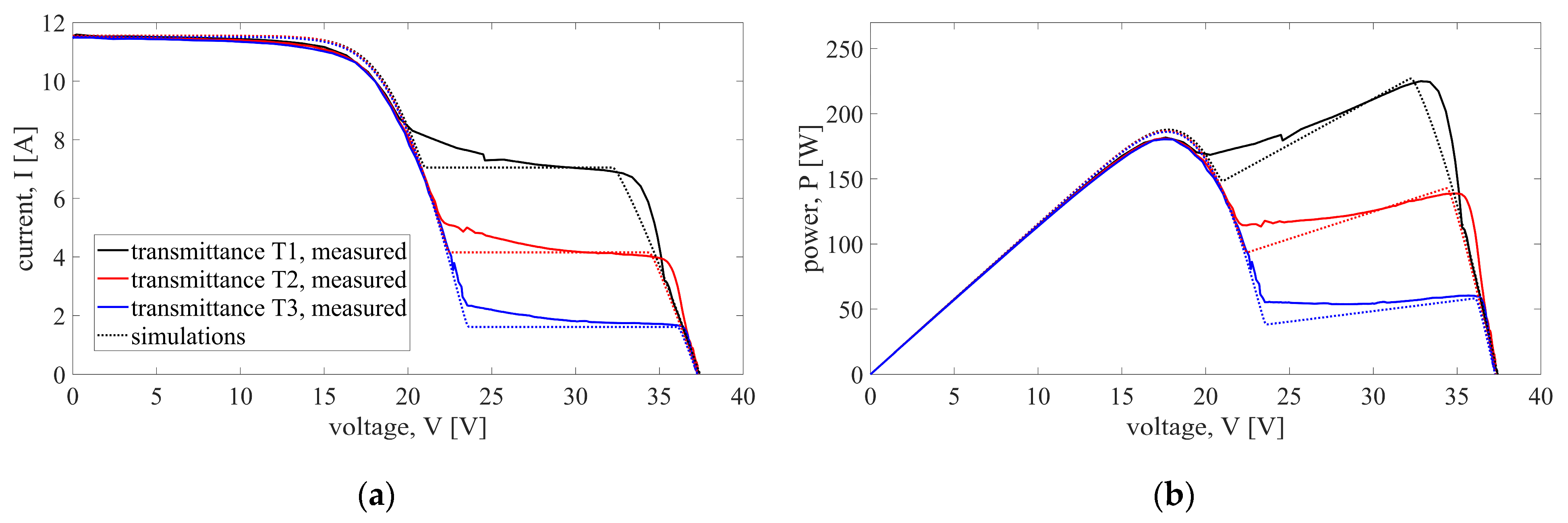
As elaborated previously, the representative scenario for this case is S11, where a single solar cell is shaded in both substrings 1A and 2A. The comparison between simulated and measured I-V and P-V curves for this scenario is shown in Figure 7. Comparison of simulations to measured I-V and P-V curves lead to the same conclusions as in Case 2: there is a clear difference around the inflection points. These points are more obvious in simulated curves, with pronounced discontinuities and more noticeable curvature changes. Measured curves exhibit more steady changes and the highest discrepancy between simulations and measurements can be seen in the region of 20 V–25 V, around the voltage when the bypass diode is activated.
The errors for Case 3 are given in Table 4. Unlike Cases 1 and 2, the simulations in Case 3 tend to overestimate the maximum power by 2.9% on average. The biggest relative error for Pm is 5.1%, but for Isc and Voc, the relative errors are 0.8% at most. The values of nRMSE for both I-V and P-V curves are higher than in Case 2, but still not surpassing 3.3% for the I-V and 5.2% for the P-V curve. Again, however, the average nRMSE for the I-V curve is smaller than for the P-V curve, suggesting a slightly better fit to the measurements. Opposite to Case 2, the largest nRMSE errors in each scenario are obtained when using the sheet with the highest transmittance, T1.

3.3. Partial Shading of Three Substrings (Cases 4 and 5)

Partial shading of three substrings is covered by Cases 4 and 5 illustrated in Figure 3. When three substrings are partially or fully shaded, as considered in Case 4, there are two possibilities: either two or all three bypass diodes are activated.
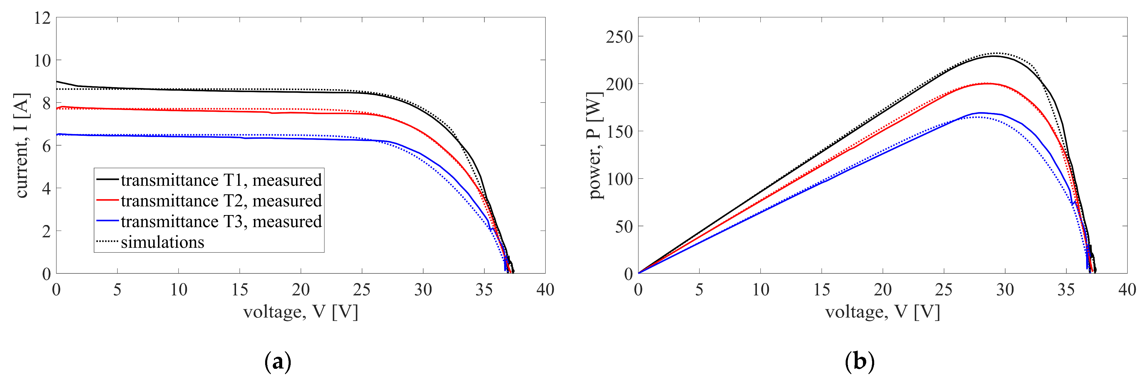
According to the notation given in Figure 2, Case 4 refers to the activation of all three bypass diodes and this happens if at least one substring of each bypass diode A, B, and C is shaded. There are eight such combinations, but for convenience the shading of all three substrings from the top half of the PV module (substrings 1A, 1B, and 1C) is chosen for analysis, denoted as Case 4 in Figure 3. This case is covered with three scenarios (S17–S19), differing only by the number of shaded solar cells in the substring. An identical number of shaded solar cells per substring is assumed in all three scenarios. The comparison for a representative scenario with a single shaded solar cell per substring (scenario S17) is shown in Figure 8. Due to the activation of all three diodes, the I-V curve looks as if the PV module is unshaded, with a major difference in the output current. The unshaded part of the module is unaffected, so the total output current is the sum of the currents produced by unshaded and shaded parts of the module. Since the current of the shaded part of the module depends on the transmittance of a shading sheet, the output current is maximum for the sheet with transmittance T1. Increasing the number of shaded solar cells per substring makes no impact on the simulation accuracy. The accuracies of simulated I-V and P-V curves are comparable, with an average nRMSE of 2.2%. The errors for Case 4 scenarios are given in Table 5. It can be seen that the simulation tends to marginally overestimate the maximum power when using sheets with higher transmittance (T1 and T2), but in all three scenarios underestimate the maximum power when the shading is achieved using sheets with transmittance T3. However, these are very modest deviations. Apart from two higher values of relative error for Isc, all other relative errors are quite small, with 87% of them having a value below 2%.
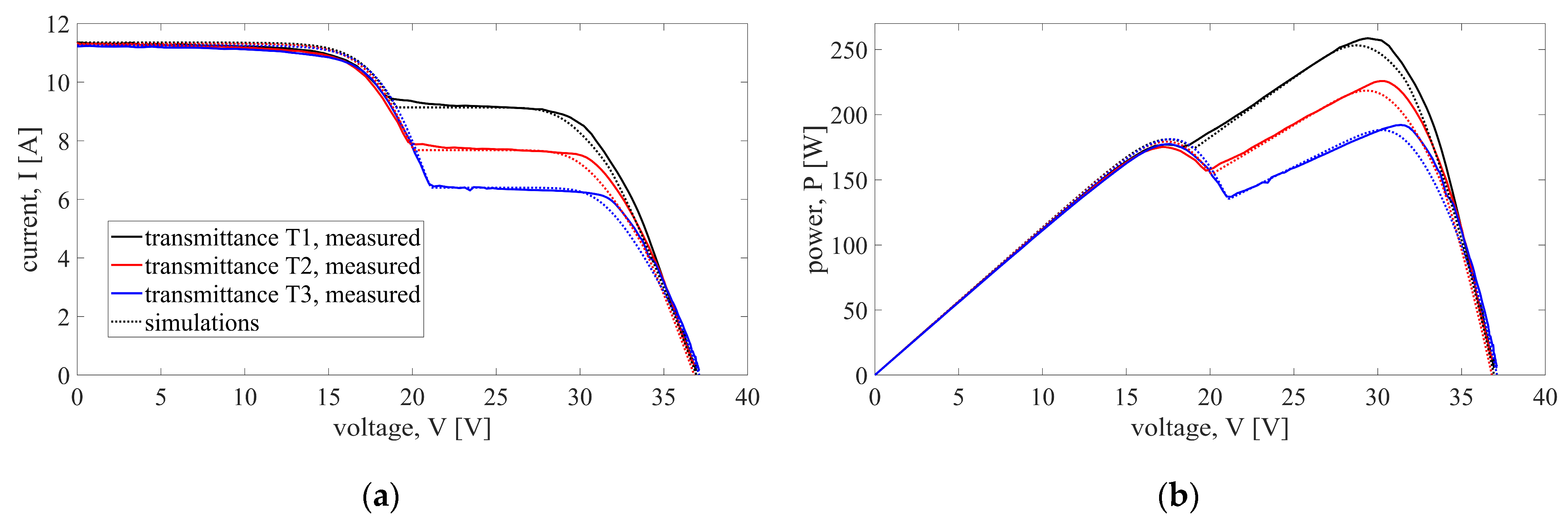
In Case 5, there are three partially shaded substrings, two of which are connected to the same bypass diode. Therefore, in scenarios belonging to this case, two bypass diodes are activated, but at different voltages. There are 12 possible combinations corresponding to this situation. Under the assumption of identical solar cells in the module and identical bypass diodes, the performance of the PV module would be the same for any of these 12 combinations. Hence, in this study, such a case is covered by three scenarios (S20–S22) for shaded substrings 1A, 2A, and 1B. In these scenarios, only an equal number of shaded solar cells per substring is considered (one, two, or five shaded solar cells per substring). All three substring pairs operate under different conditions: both substrings connected to bypass diode A are partially shaded, one substring connected to bypass diode B is partially shaded and the other one is fully illuminated, while both substring pairs sharing bypass diode C are fully illuminated. As a result of such an imbalance, the I-V curve exhibits a cascade form, as shown in Figure 9a. Here, the discrepancy between simulation and measurement is more obvious and it can be observed along most of the curve. The most notable differences are in the slope of the I-V curve and the curvature near the voltages where bypass diodes are activated. While simulations predict an almost constant current for a particular voltage region and sharp transitions between the regions, the measured current decreases much more gently along the entire voltage range. The higher the transmittance of a shading sheet, the bigger the difference between simulated and measured curves. In other words, weaker shading results in a smoother I-V curve, with less pronounced curvature changes. Despite the described differences, the nRMSE values are pretty low in all scenarios, having a maximum of 4.1% and a mean of 2.8%. However, the errors are somewhat higher when the P-V curve is analyzed. With all three substring pairs operating under different conditions, it is expected that the P-V curve has three maximum points, just as can be seen on the simulated curves in Figure 9b. Interestingly, the curve measured using the weakest shade (sheet with transmittance T1) practically exhibits only one maximum point. This behavior is already observed in Case 2; see Figure 6b. Another interesting observation is related to the magnitudes of maximum points. For medium shading, using a sheet with transmittance T2, the two highest local maximum points are very close (red curve in Figure 9b) and the simulation faulty calculated the global maximum power point. The measured maximum power point occurs at 19 V, and in simulations the maximum power point occurs at 34.2 V. As a result, very large relative errors are obtained for Vm and Im in scenario S20, using the T2 sheet. The aforementioned situation is extremely important for maximum power point tracking, and special care should be taken when the magnitudes of local and global maximum become close. Same as in previous cases, the accuracy of simulated P-V curves is slightly lower than that of the I-V curves, with an average nRMSE of 4.5%, and maximum nRMSE of 5.8%. The errors for Case 5 scenarios are given in Table 6. Apart from the already mentioned larger errors, most of the error values are within ±3%. One more interesting thing to note is that nMBE errors for the I-V curve tend to be positive, unlike nMBE errors for the P-V curve which are mostly negative.
Although in both Case 4 and Case 5 an equal number of partially shaded substrings is considered, the simulation accuracy for Case 4 is a little higher. A similar reduction in model accuracy when both substrings are connected to the same diode are shaded is also observed in results presented in Section 3.2: both Case 2 and Case 3 consider scenarios when two substrings are partially shaded, but Case 3 (when both substrings are connected to the same bypass diode) exhibits somewhat lower overall accuracy compared to Case 2.

3.4. Additional Comparison of Studied Cases of Partial Shading

As seen from the results presented for the five studied cases, there is a high level of agreement between simulated and measured PV module output characteristics under different shading conditions. Further analysis investigates the dependency of the simulation accuracy on the number of shaded substrings, the number of shaded solar cells, and the shading intensity.
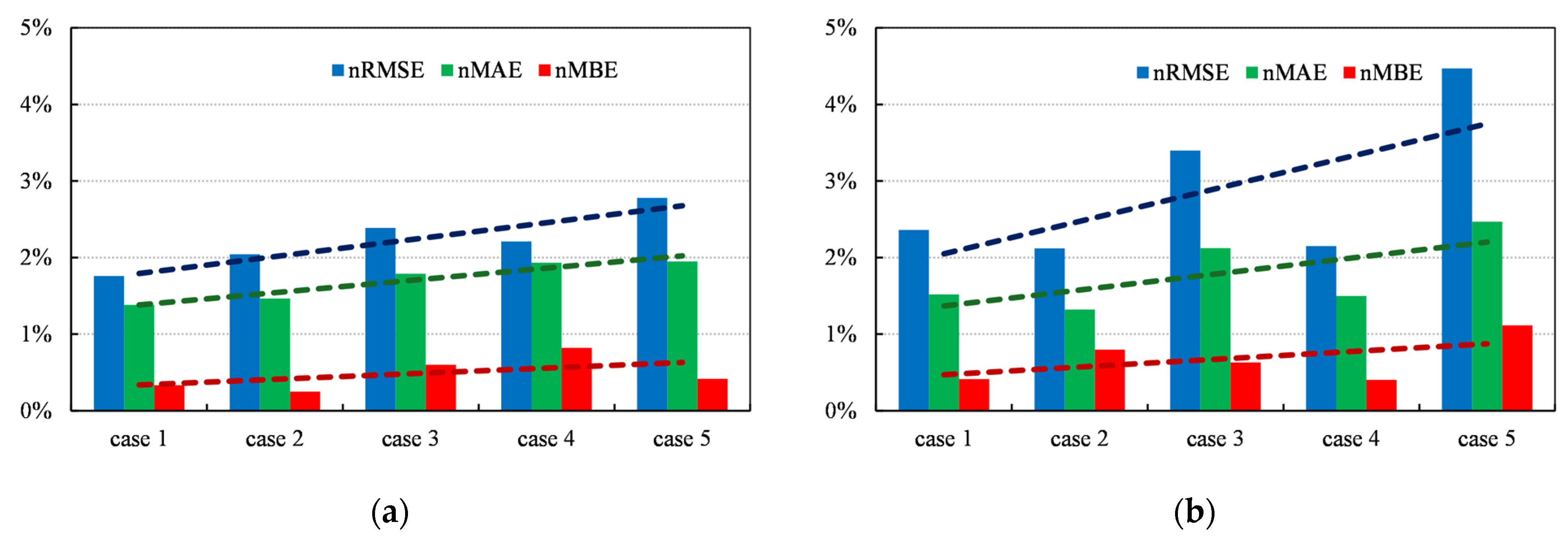
The comparison of the accuracy by Cases 1–5 is based on the mean values of nRMSE, nMAE, and nMBE for I-V and P-V curves. As already mentioned, nMBE is calculated using absolute nMBE values for every shading scenario and shading level. The results are shown in Figure 10. It is evident that for both the I-V and P-V curves, all three error metrics tend to increase from Case 1 to Case 5. Also, the errors for P-V curves are slightly bigger when compared to I-V curves. To detect the main cause of the observed trend, further analysis focuses on the number of shaded solar cells. Yet, no obvious relation between the simulation accuracy and the total number of shaded solar cells is found. Similarly, it is found that the transmittance of the shading sheet makes no impact on the simulation accuracy. Therefore, one can conclude that the main parameter influencing the accuracy of the evaluated model is the number of shaded substrings: errors increase with the number of shaded substrings. Additionally, it seems that the simulation accuracy is lower in cases when both substrings sharing the same bypass diode are partially shaded.
While the presented research considers only up to three partially shaded substrings, the results indicate that the accuracy of the Simscape solar cell model might slightly decrease if even more substrings are shaded. However, current data show that the biggest deviation from measurements occurs for Case 5, when all three substring pairs operate under different conditions. Scenarios with four to six shaded substrings would certainly include shading at least one pair that shares the same bypass diode, possibly negatively affecting the model accuracy. However, in these cases, at least two bypass diodes would operate in the same conditions, so the overall imbalance is lesser than in Case 5. Therefore, for a definitive answer, additional research needs to be performed.

4. Discussion

The presented results confirm that the output curves of the partially shaded half-cut PV module can be accurately modeled by using the simplest five-parameter Simscape solar cell block. The model is validated across a variety of partial shading scenarios, with the average nRMSE for I-V curves of 2.2% ± 0.15% at the 95% confidence interval. The accuracy is a bit lower for P-V curves, with the mean nRMSE of 2.8% ± 0.3% at the 95% confidence interval. All other error metrics in all 22 scenarios and for the three considered shading levels are typically within ±5%. Error analysis shows that the simulation accuracy depends on the number of shaded substrings, but is independent of the number of shaded solar cells and the shading level. As seen from the results of scenario S1 when the sheet with transmittance T1 is used, even the smallest shade is enough to activate the bypass diode. Increasing the area or shade intensity of the shaded substring (substring 1A) would just confirm the bypassing of this substring. The errors tend to increase when multiple inflection points exist as a result of the partial shading of the multiple substrings.
Despite low error values in most of the studied scenarios, some typical deviations between simulated and measured curves can be noted. This primarily concerns the slope of the I-V curve, which is horizontal in simulations until the inflection points are reached, while on most measured I-V curves a steady decrease in current can be noted even between the inflection points. The decrease in the measured current and consequently the increase in simulation errors are especially noticeable in Cases 3 and 5. Both of these cases comprise scenarios where both substrings connected to the same bypass diode are shaded. The voltage region where the greatest discrepancy between simulations and measurements occurs (before or after the inflection point of the I-V curve) depends on the shading pattern. For scenarios belonging to Case 2, this region is between 0 V and 10 V, close to the first inflection point. On the other hand, in Case 3 scenarios, the errors are the most noticeable after the inflection point (after 23 V). Finally, the biggest errors for Case 5 occur before the first and after the second inflection point.
As reported in [40], the slope of the measured I-V curve slightly decreases when increasing the number of shaded solar cells in a substring. Still, simulated I-V curves exhibit nearly constant current in the voltage region between inflection points regardless of the shaded area. To account for this, the addition of shunt resistance to the solar cell model might be suitable. In Simulink, this is only possible by using the double-diode model with eight parameters where additional parameters with unknown values are introduced. Then, much more computation is needed to determine these parameters. However, given the high accuracy of the simplest model, the benefits of using a more complex model are limited.
The accuracy of the model in simulating P-V curves is somewhat lower than for I-V curves. The differences mainly occur in the vicinity of the local and global maxima. Same as with I-V curves, increasing the number of shaded substrings results in greater errors. In some scenarios, at a low shading level, there is a specific mismatch between simulated and measured P-V curves. While simulated curves exhibit multiple maxima, in measured curves, only a single (global) maximum is evident. Additionally, it should be noted that in conditions when global and local maximum power have similar values, the simulations might wrongly choose the global maximum (red line in Figure 9b).

5. Conclusions

The simplest form of the often-used MATLAB Simscape (MATLAB R2023a with Simulink v. 10.7 was used) solar cell block is validated against measured data for modeling the half-cut PV module in partially shaded conditions.
  • A great number of shading scenarios is taken into account, designed by varying
    -
    shaded module area corresponding to different numbers of shaded solar cells,
    -
    distribution of shaded area covering from one to three solar cell substrings in different configurations,
    -
    shading intensity.
    In total, 66 unique shading conditions are considered.
  • Comprehensive error metrics for evaluation of the model’s accuracy are proposed that not only take into account the characteristic points (Pm, Isc, Voc), but also assess the accuracy of the whole I-V and P-V curves generated by the model for a given shading condition.
  • The simulation results are compared to the measurements on a partially shaded half-cut PV module. Comparisons show a great level of agreement between simulations and measurements, with errors being limited to ±3% in most shading conditions and for most considered metrics.
  • Comparisons of errors between different scenarios show that model errors depend mostly on the shadow distribution on the module (i.e., number and configuration of partially shaded substrings), while the variations in the number of shaded cells and shading intensity have limited influence on errors. However, more extensive simulations and measurements are needed to be able to statistically determine and quantify how the change in one of these parameters (shadow distribution, area, and intensity) influences the model’s accuracy.

Author Contributions

Conceptualization, T.B. and A.K.; methodology, T.B. and A.K.; software, T.B., A.K. and V.P.; validation, I.M. and V.P.; formal analysis, T.B. and A.K.; investigation, T.B. and A.K.; resources, T.B. and I.M.; data curation, T.B. and I.M.; writing—original draft preparation, T.B. and A.K.; writing—review and editing, I.M. and V.P.; visualization, I.M. and V.P.; supervision, T.B. All authors have read and agreed to the published version of the manuscript.

Funding

This research received no external funding.

Data Availability Statement

The original contributions presented in the study are included in the article, further inquiries can be directed to the corresponding author.

Conflicts of Interest

The authors declare no conflicts of interest.

References

  1. Patel, H.; Agarwal, V. MATLAB-Based Modeling to Study the Effects of Partial Shading on PV Array Characteristics. IEEE Trans. Energy Convers. 2008, 23, 302–310. [Google Scholar] [CrossRef]
  2. Abdulmawjood, K.; Alsadi, S.; Refaat, S.S.; Morsi, W.G. Characteristic Study of Solar Photovoltaic Array under Different Partial Shading Conditions. IEEE Access 2022, 10, 6856–6866. [Google Scholar] [CrossRef]
  3. Nguyen, X.H. Matlab/Simulink Based Modeling to Study Effect of Partial Shadow on Solar Photovoltaic Array. Environ. Syst. Res. 2015, 4, 20. [Google Scholar] [CrossRef]
  4. Meyers, B.; Mikofski, M. Accurate Modeling of Partially Shaded PV Arrays. In Proceedings of the 2017 IEEE 44th Photovoltaic Specialist Conference (PVSC), Washington, DC, USA, 25–30 June 2017; pp. 3354–3359. [Google Scholar]
  5. Mäki, A.; Valkealahti, S.; Leppäaho, J. Operation of Series-Connected Silicon-Based Photovoltaic Modules under Partial Shading Conditions. Prog. Photovolt. Res. Appl. 2012, 20, 298–309. [Google Scholar] [CrossRef]
  6. Rauschenbach, H.S. Electrical Output of Shadowed Solar Arrays. IEEE Trans. Electron Devices 1971, 18, 483–490. [Google Scholar] [CrossRef]
  7. Bowden, S.; Honsberg, C. PVCDROM | PVEducation. Available online: https://www.pveducation.org (accessed on 28 April 2024).
  8. Petrone, G.; Ramos-Paja, C.A.; Spagnuolo, G. Photovoltaic Sources Modeling; John Wiley & Sons: Hoboken, NJ, USA, 2017; ISBN 978-1-118-67903-6. [Google Scholar]
  9. Mertens, K. Photovoltaics: Fundamentals, Technology, and Practice; John Wiley & Sons: Hoboken, NJ, USA, 2018; ISBN 978-1-119-40104-9. [Google Scholar]
  10. Cotfas, D.T.; Cotfas, P.A.; Kaplanis, S. Methods to Determine the Dc Parameters of Solar Cells: A Critical Review. Renew. Sustain. Energy Rev. 2013, 28, 588–596. [Google Scholar] [CrossRef]
  11. Jordehi, A.R. Parameter Estimation of Solar Photovoltaic (PV) Cells: A Review. Renew. Sustain. Energy Rev. 2016, 61, 354–371. [Google Scholar] [CrossRef]
  12. Oulcaid, M.; El Fadil, H.; Ammeh, L.; Yahya, A.; Giri, F. Parameter Extraction of Photovoltaic Cell and Module: Analysis and Discussion of Various Combinations and Test Cases. Sustain. Energy Technol. Assess. 2020, 40, 100736. [Google Scholar] [CrossRef]
  13. Gu, Z.; Xiong, G.; Fu, X. Parameter Extraction of Solar Photovoltaic Cell and Module Models with Metaheuristic Algorithms: A Review. Sustainability 2023, 15, 3312. [Google Scholar] [CrossRef]
  14. Batzelis, E.I.; Georgilakis, P.S.; Papathanassiou, S.A. Energy Models for Photovoltaic Systems under Partial Shading Conditions: A Comprehensive Review. IET Renew. Power Gener. 2015, 9, 340–349. [Google Scholar] [CrossRef]
  15. Gow, J.A.; Manning, C.D. Development of a Photovoltaic Array Model for Use in Power-Electronics Simulation Studies. IEE Proc.-Electr. Power Appl. 1999, 146, 193–200. [Google Scholar] [CrossRef]
  16. Boukenoui, R.; Salhi, H.; Bradai, R.; Mellit, A. A New Intelligent MPPT Method for Stand-Alone Photovoltaic Systems Operating under Fast Transient Variations of Shading Patterns. Sol. Energy 2016, 124, 124–142. [Google Scholar] [CrossRef]
  17. Chellaswamy, C.; Ramesh, R. Future Renewable Energy Option for Recharging Full Electric Vehicles. Renew. Sustain. Energy Rev. 2017, 76, 824–838. [Google Scholar] [CrossRef]
  18. Verma, D.; Nema, S.; Nema, R.K. Implementation of Perturb and Observe Method of Maximum Power Point Tracking in SIMSCAPE/MATLAB. In Proceedings of the 2017 International Conference on Intelligent Sustainable Systems (ICISS), Palladam, India, 7–8 December 2017; pp. 148–152. [Google Scholar]
  19. Brown, R.; Kamper, M.J.; Ockhuis, D.K. Utility-Scale PV-Powered Motor-Generator System with Model-Based MPPT Control. In Proceedings of the 2023 International Aegean Conference on Electrical Machines and Power Electronics (ACEMP) & 2023 International Conference on Optimization of Electrical and Electronic Equipment (OPTIM), Istanbul, Türkiye, 1–2 September 2023; pp. 1–8. [Google Scholar]
  20. Orta-Quintana, Á.A.; García-Chávez, R.E.; Silva-Ortigoza, R.; Marciano-Melchor, M.; Villarreal-Cervantes, M.G.; García-Sánchez, J.R.; García-Cortés, R.; Silva-Ortigoza, G. Sensorless Tracking Control Based on Sliding Mode for the “Full-Bridge Buck Inverter–DC Motor” System Fed by PV Panel. Sustainability 2023, 15, 9858. [Google Scholar] [CrossRef]
  21. Lu, F.; Guo, S.; Walsh, T.M.; Aberle, A.G. Improved PV Module Performance under Partial Shading Conditions. Energy Procedia 2013, 33, 248–255. [Google Scholar] [CrossRef]
  22. Brecl, K.; Bokalič, M.; Topič, M. Annual Energy Losses Due to Partial Shading in PV Modules with Cut Wafer-Based Si Solar Cells. Renew. Energy 2021, 168, 195–203. [Google Scholar] [CrossRef]
  23. Qian, J.; Thomson, A.; Blakers, A.; Ernst, M. Comparison of Half-Cell and Full-Cell Module Hotspot-Induced Temperature by Simulation. IEEE J. Photovolt. 2018, 8, 834–839. [Google Scholar] [CrossRef]
  24. Trends in PV Applications 2023. Available online: https://iea-pvps.org/trends_reports/trends-2023/ (accessed on 20 March 2024).
  25. Yang, Z.; Liao, K.; Chen, J.; Xia, L.; Luo, X. Output Performance Analysis and Power Optimization of Different Configurations Half-Cell Modules under Partial Shading. Optik 2021, 232, 166499. [Google Scholar] [CrossRef]
  26. Sarniak, M.T. Modeling the Functioning of the Half-Cells Photovoltaic Module under Partial Shading in the Matlab Package. Appl. Sci. 2020, 10, 2575. [Google Scholar] [CrossRef]
  27. Quaschning, V.; Hanitsch, R. Influence of Shading on Electrical Parameters of Solar Cells. In Proceedings of the Conference Record of the Twenty Fifth IEEE Photovoltaic Specialists Conference—1996, Washington, DC, USA, 13–17 May 1996; pp. 1287–1290. [Google Scholar]
  28. Wang, Y.; Pei, G.; Zhang, L. Effects of Frame Shadow on the PV Character of a Photovoltaic/Thermal System. Appl. Energy 2014, 130, 326–332. [Google Scholar] [CrossRef]
  29. Bharadwaj, P.; John, V. Subcell Modeling of Partially Shaded Photovoltaic Modules. IEEE Trans. Ind. Appl. 2019, 55, 3046–3054. [Google Scholar] [CrossRef]
  30. Moreira, H.S.; Lucas de Souza Silva, J.; Gomes dos Reis, M.V.; de Bastos Mesquita, D.; Kikumoto de Paula, B.H.; Villalva, M.G. Experimental Comparative Study of Photovoltaic Models for Uniform and Partially Shading Conditions. Renew. Energy 2021, 164, 58–73. [Google Scholar] [CrossRef]
  31. MS-711N Spectroradiometer. Available online: https://www.eko-instruments.com/cn/categories/products/spectroradiometers/ms-711n-spectroradiometer (accessed on 1 April 2024).
  32. Singh, A.; Umakanth, V.; Tyagi, N.; Baghel, A.K.; Kumar, S. Comparative Study of Commercial Crystalline Solar Cells. Results Opt. 2023, 11, 100379. [Google Scholar] [CrossRef]
  33. Solvis SV120 E HC9B Datasheet. Available online: https://solvis.hr/wp-content/uploads/2022/03/LQSOLVIS-DS-EN-SV120_E_HC9B-1755x1038x35-355-375-20210222.pdf (accessed on 29 April 2024).
  34. MP-11 Portable I–V Checker. Available online: https://www.eko-instruments.com/eu/categories/products/i-v-measurement-instruments/mp-11-portable-i-v-checker (accessed on 21 March 2024).
  35. Photovoltaic Solar Cell—MATLAB. Available online: https://www.mathworks.com/help/sps/ref/solarcell.html (accessed on 29 April 2024).
  36. Marion, B.; Kroposki, B.; Emery, K.; Cueto, J.; Myers, D.; Osterwald, C. Validation of a Photovoltaic Module Energy Ratings Procedure at NREL; NREL/TP-520-26909; NREL Technical Report; National Renewable Energy Laboratory (NREL): Golden, CO, USA, 1999. [CrossRef]
  37. Cubas, J.; Pindado, S.; Sorribes-Palmer, F. Analytical Calculation of Photovoltaic Systems Maximum Power Point (MPP) Based on the Operation Point. Appl. Sci. 2017, 7, 870. [Google Scholar] [CrossRef]
  38. Jadli, U.; Thakur, P.; Shukla, R.D. A New Parameter Estimation Method of Solar Photovoltaic. IEEE J. Photovolt. 2018, 8, 239–247. [Google Scholar] [CrossRef]
  39. Peña, R.; Diez-Pascual, A.M.; Díaz, P.G.; Davoise, L.V. A New Method for Current–Voltage Curve Prediction in Photovoltaic Modules. IET Renew. Power Gener. 2021, 15, 1331–1343. [Google Scholar] [CrossRef]
  40. Alonso-García, M.C.; Ruiz, J.M.; Herrmann, W. Computer Simulation of Shading Effects in Photovoltaic Arrays. Renew. Energy 2006, 31, 1986–1993. [Google Scholar] [CrossRef]
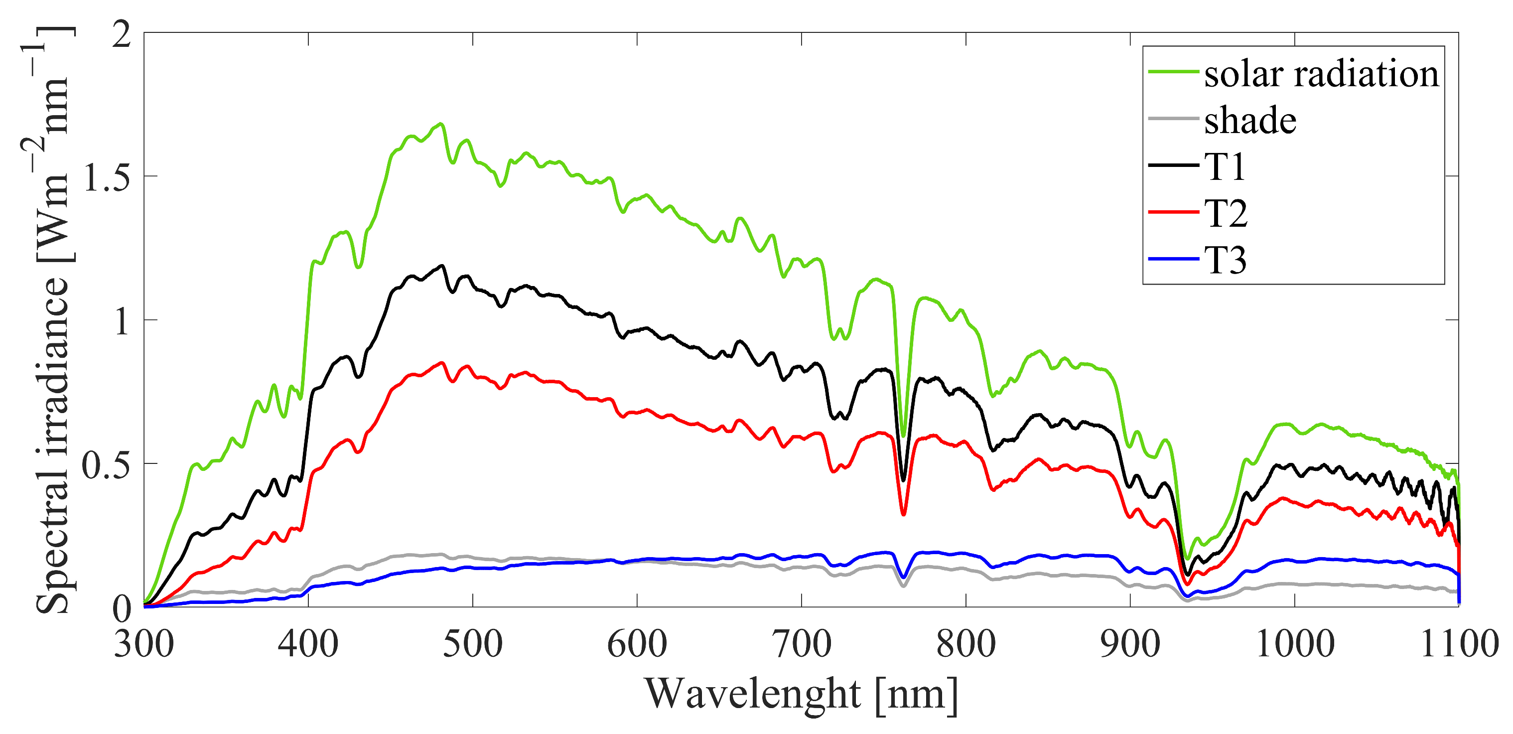
Figure 1. The measured spectra of the shading sheets with transmittances T1–T3 compared to the unshaded spectrum. Also, the spectrum of the “regular” shade is presented, measured when the spectroradiometer is shaded by the shading object (here, cardboard placed approximately 1 m away from the instrument is used for shading).
Energies 17 02276 g001
Figure 2. (a) The structure of the half-cut PV module under study, with labeled substrings; (b) The main parameters of the PV module.
Energies 17 02276 g002
Figure 3. Considered cases of shading scenarios, denoted S1–S22 in the figure. Shaded blocks indicate the position of the shaded substrings and numbers on the shaded blocks indicate the number of shaded cells in the corresponding substring. For every scenario, all three shading levels corresponding to sheets having transmittances T1–T3 are examined.
Energies 17 02276 g003
Figure 4. Comparison of simulations and measurements for the case of an unshaded PV module (referent scenario S0): (a) I-V curve; (b) P-V curve.
Energies 17 02276 g004
Figure 5. Comparison of simulations and measurements for Case 1, when only one solar cell in the PV module is shaded (shading of substring 1A, scenario S1): (a) I-V curve; (b) P-V curve. The measurements are shown with full lines, and dotted lines represent curves obtained by simulations.
Energies 17 02276 g005
Figure 6. Comparison of simulations and measurements for Case 2, when a single solar cell is shaded in each of two substrings connected to different bypass diodes (shading of substrings 1A and 1B, scenario S5): (a) I-V curve; (b) P-V curve. The measurements are shown with full lines, and dotted lines represent curves obtained by simulations.
Energies 17 02276 g006
Figure 7. Comparison of simulations and measurements for Case 3, when a single solar cell is shaded in both substrings connected to the same bypass diode (shading of substrings 1A and 2A, scenario S11): (a) I-V curve; (b) P-V curve. The measurements are shown with full lines, and dotted lines represent curves obtained by simulations.
Energies 17 02276 g007
Figure 8. Comparison of simulations and measurements for Case 4, when a single solar cell per substring is shaded in the top half of the PV module (shading of substrings 1A, 1B, and 1C, scenario S17): (a) I-V curve; (b) P-V curve. The measurements are shown with full lines, and dotted lines represent curves obtained by simulations.
Energies 17 02276 g008
Figure 9. Comparison of simulations and measurements for Case 5 with three partially shaded substrings, one shaded solar cell per substring, and two substrings connected to the same bypass diode (shading of substrings 1A, 2A, and 1B, scenario S20): (a) I-V curve; (b) P-V curve. The measurements are shown with full lines, and dotted lines represent curves obtained by simulations.
Energies 17 02276 g009
Figure 10. Comparison of error metrics by studied shading cases: (a) error metrics for I-V curves; (b) error metrics for the P-V curves. Dashed lines represent trendlines obtained by linear regression.
Energies 17 02276 g010
Table 1. Overall errors for all scenarios. Error values are given as percentages (%). The errors for scenario S0 are given as a reference.
Relative Error XrelI-V CurveP-V Curve
PmVmImVocIscnRMSEnMAEnMBEnRMSEnMAEnMBE
S00.73.12.50.80.010.70.60.50.60.50.5
S1–S22Mean2.23.22.50.50.92.21.70.52.81.80.7
Max5.180.5−43.41.93.54.54.21.85.83.5−2.3
Table 2. Errors for Case 1 scenarios (S1–S4). Error values are given as percentages (%).
Relative Error XrelI-V CurveP-V Curve
ScenarioShading LevelPmVmImVocIscnRMSEnMAEnMBEnRMSEnMAEnMBE
S1T1−2.1−2.30.10.80.11.71.3−0.22.11.3−0.7
T2−3.3−3.1−0.2−0.30.11.91.5−0.22.81.7−0.9
T3−2.1−3.71.8−0.10.31.71.30.32.71.7−0.3
S2T1−2.5−1.6−0.9−1.3−0.11.51.00.11.61.0−0.3
T2−1.4−3.32.0−0.10.21.71.30.52.01.40.1
T3−1.6−3.41.9−1.40.31.71.30.42.61.7−0.1
S3T1−2.3−2.40.10.00.21.41.00.11.50.9−0.3
T2−2.8−2.80.01.00.61.91.50.22.51.6−0.5
T3−1.6−2.81.31.90.71.91.60.52.91.9−0.2
S4T1−2.2−2.70.50.40.72.11.60.12.51.5−0.6
T2−0.4−2.52.10.30.81.71.41.01.71.30.6
T3−1.2−4.23.10.7−3.22.01.60.33.52.1−0.4
Table 3. Errors for Case 2 scenarios (S5–S10). Error values are given as percentages (%).
Relative Error XrelI-V CurveP-V Curve
ScenarioShading LevelPmVmImVocIscnRMSEnMAEnMBEnRMSEnMAEnMBE
S5T1−1.61.2−2.80.00.92.11.6−0.31.51.0−0.7
T2−2.1−0.1−2.0−1.70.71.91.30.11.10.8−0.2
T3−4.7−3.4−1.30.41.42.61.9−0.53.01.9−1.4
S6T1−1.21.1−2.3−0.1−0.21.71.30.11.10.8−0.4
T2−2.0−0.5−1.5−1.2−1.41.71.2−0.11.71.1−0.7
T3−4.7−2.5−2.20.11.42.81.9−0.53.32.0−1.5
S7T1−2.7−0.7−2.0−0.51.62.41.8−0.52.91.6−1.4
T2−0.90.9−1.81.10.31.51.00.30.90.6−0.1
T3−2.8−2.2−0.6−0.71.52.72.0−0.13.52.2−1.1
S8T1−3.3−0.1−3.1−0.50.52.21.7−0.72.51.5−1.3
T2−2.6−0.8−1.7−1.7−0.32.01.4−0.22.31.3−1.0
T3−3.1−2.6−0.50.10.71.91.40.12.01.4−0.6
S9T1−1.11.1−2.3−0.3−0.21.91.30.01.81.0−0.7
T2−1.3−0.7−0.6−0.4−5.91.61.00.31.00.7−0.2
T3−4.0−3.3−0.6−0.4−0.12.31.6−0.43.52.1−1.3
S10T1−1.80.8−2.6−1.1−0.51.61.10.11.20.8−0.5
T2−2.0−0.6−1.40.0−0.11.71.2−0.01.81.1−0.6
T3−3.3−2.8−0.6−0.40.62.11.70.13.02.0−0.8
Table 4. Errors for Case 3 scenarios (S11–S16). Error values are given as percentages (%).
Relative Error XrelI-V CurveP-V Curve
ScenarioShading LevelPmVmImVocIscnRMSEnMAEnMBEnRMSEnMAEnMBE
S11T10.9−1.92.80.20.13.32.2−0.74.62.6−1.4
T23.20.92.20.00.33.02.2−0.35.23.0−1.3
T33.20.72.40.10.52.42.0−0.13.52.7−1.1
S12T1−1.1−2.61.60.30.42.61.80.13.82.0−0.6
T23.54.3−0.70.40.32.01.50.53.41.90.0
T34.10.73.4−0.20.61.91.60.62.41.90.1
S13T1−2.2−3.31.20.00.12.81.8−0.64.62.3−1.5
T24.01.52.50.70.22.01.50.53.41.9−0.1
T33.01.41.5−0.50.41.81.40.62.21.60.1
S14T1−0.3−3.12.9−0.30.72.92.3−0.13.92.6−0.9
T24.31.82.40.70.62.72.10.43.72.7−0.2
T34.21.92.2−0.50.72.21.80.62.72.00.1
S15T1−1.9−3.21.3−0.20.62.51.80.43.31.9−0.3
T23.21.02.20.30.62.01.50.83.11.90.3
T34.80.74.00.20.72.11.51.22.41.51.0
S16T1−0.6−3.12.50.60.82.51.90.73.52.0−0.1
T25.14.40.70.60.72.51.81.63.22.11.6
T33.02.20.70.00.61.81.51.02.31.60.7
Table 5. Errors for Case 4 scenarios (S17–S19). Error values are given as percentages (%).
Relative Error XrelI-V CurveP-V Curve
ScenarioShading LevelPmVmImVocIscnRMSEnMAEnMBEnRMSEnMAEnMBE
S17T11.41.5−0.10.0−4.11.61.30.21.61.00.2
T20.2−0.81.0−0.2−0.31.41.10.61.30.80.3
T3−2.7−0.5−2.20.20.03.02.3−0.33.52.3−1.0
S18T11.81.00.80.80.91.91.70.91.91.40.4
T20.0−1.51.5−0.41.32.01.70.82.01.20.1
T3−1.9−1.8−0.1−0.61.42.72.50.62.72.0−0.4
S19T12.02.2−0.20.21.21.51.51.21.21.00.6
T20.5−0.20.70.31.11.31.21.00.90.70.5
T3−0.9−1.50.6−1.03.54.54.21.84.23.00.0
Table 6. Errors for Case 5 scenarios (S20–S22). Error values are given as percentages (%).
Relative Error XrelI-V CurveP-V Curve
ScenarioShading LevelPmVmImVocIscnRMSEnMAEnMBEnRMSEnMAEnMBE
S20T10.9−4.15.1−1.30.94.12.9−1.05.83.2−2.3
T22.180.5−43.4−0.10.42.82.10.25.03.2−1.0
T3−0.3−2.42.1−0.51.22.72.2−0.35.03.5−2.2
S21T1−0.9−3.72.8−1.92.53.12.10.34.22.0−0.9
T21.2−1.02.3−0.51.32.31.60.64.32.0−0.4
T3−0.8−3.12.4−0.3−1.82.11.50.72.41.80.3
S22T1−2.4−4.62.3−2.2−0.43.11.9−0.24.92.2−1.5
T20.1−2.32.4−0.82.12.71.80.15.72.5−1.3
T31.3−0.41.7−0.30.62.11.50.42.91.8−0.2
Disclaimer/Publisher’s Note: The statements, opinions and data contained in all publications are solely those of the individual author(s) and contributor(s) and not of MDPI and/or the editor(s). MDPI and/or the editor(s) disclaim responsibility for any injury to people or property resulting from any ideas, methods, instructions or products referred to in the content.