Closed-Form Expressions for Local Absorbing Boundary Conditions in Electromagnetic Scattering Problems and Their Implementation into Commercial FEM Software

Abstract

When solving open-region electromagnetic scattering problems using the standard finite element method, the infinite region exterior to the scatterer must be truncated with an artificial outer boundary. In the interior or finite part of the domain, finite elements can be used, but a boundary condition must be introduced at this artificial boundary to obtain a unique finite element solution. One class of boundary conditions designed for this purpose is called absorbing boundary conditions (ABCs). Several ABCs have been reported in the literature. These can be broadly classified into two categories: local and non-local. In this paper, we present new closed-form expressions for Nth-order local ABCs, equivalent to the well-known sequences of the Bayliss, Gunzburger, and Turkel boundary operators. To the best of our knowledge, these expressions have not yet been reported in the literature. Two- and three-dimensional problems are considered in this study. We also discuss the problem of incorporating custom ABCs into commercial finite element method programs, which are usually closed-source software packages. Two 2D electromagnetic scattering and radiation problems with known analytical solutions are analyzed.

1. Introduction

The solution domain in exterior electromagnetic scattering problems can be seen as bounded at infinity. When solving such problems using the finite element method (FEM), the unbounded region exterior to the scatterer must be truncated with an artificial outer boundary to limit the size of the computational domain [1]. In the finite part of the domain, finite elements can be used, but special procedures must be adopted for the part of the domain extending to infinity. A number of different approaches to this problem have been proposed, studied, and implemented, such as infinite elements [2,3,4], perfectly matched layers (PMLs) [5], and absorbing boundary conditions (ABCs, sometimes called radiation boundary conditions or scattering boundary conditions) [6]. Such conditions must be imposed on the artificial outer boundary such that it appears as close to transparent as possible for the electromagnetic waves impinging upon it from the interior. Obviously, in the asymptotic limit where the outer boundary tends to infinity, the ABCs should become identical to the Silver–Müller radiation conditions [7].

Several ABCs have been reported in the literature. These can be broadly classified into two categories, viz., global or non-local and local. The global boundary conditions are exact and allow one to bring in the outer boundary as close to the scatterer as desired, but they result in full matrices generated via FEM that are computationally expensive [8,9]. In contrast, local ABCs retain the sparse structure of the finite element formulation and, consequently, are highly attractive from a numerical point of view. However, local ABCs are not exact in their truncated asymptotic form and introduce errors in the solution because of the presence of reflecting waves from the artificial outer boundary [10].

A number of authors have investigated local ABCs for two- and three-dimensional electromagnetic scattering problems over the years. The most notable local ABCs were proposed by Bayliss, Gunzburger, and Turkel, who employed a Wilcox-type expansion for the scattered fields to derive a series of local boundary operators (BGT operators) [11,12,13,14,15,16]. In [17], a local ABC was developed for two-dimensional electromagnetic scattering using a modal expansion basis function. Formulations with circular and non-circular boundaries were considered. Different formulations of absorbing boundary conditions are given in [18,19,20,21,22].

In this paper, we present closed-form, previously unknown (to the best knowledge of the authors of this paper), general expressions for Nth-order local ABCs, for both two- and three-dimensional electromagnetic scattering problems, which are equivalent to the BGT operators. In the second section of this paper, we show the equivalence of the BGT boundary operators and our alternative versions in the form of general expressions for Nth-order local ABCs.

The implementation of ABCs in finite element method programs is relatively simple if the source code of the program is available. In the third section of this paper, we show that in the RF module of COMSOL Multiphysics it is sufficient to select the so-called surface current density boundary conditions to introduce custom conditions on the artificial outer boundary of the finite element region [23]. The ABCs for cylindrical coordinates (two-dimensional problems) and spherical coordinates (three-dimensional problems) are written in the form of the surface current density and presented in Cartesian coordinates. Sections four and five present two test electromagnetic scattering and radiation problems introducing local ABCs on the outer artificial boundary via the surface current density boundary condition.

2. Local Absorbing Boundary Conditions

Consider a scattering problem in which an incident electromagnetic wave with harmonic time dependence is intercepted by a scatterer. It is convenient to regard the total wavefunction at any point as comprising two parts: a known incident wave and a scattered wave that has to be determined. In three dimensions, for a linear, isotropic, homogeneous, and source-free medium, the electric and magnetic field vectors E and H satisfy the wave equation (scattered/radiated fields):

$$\left({\nabla }^2+k^2\right)\left(\begin{array}{c}\underset{¯}{E}\\ \underset{¯}{H}\end{array}\right)=0,$$

(1)

where time factor exp(jωt) is omitted, $k=\omega \sqrt{\epsilon \mu }=2\mathrm{\pi }/\lambda$ is the wave number, ω is the circular driving frequency, λ is the wavelength, ε is the permittivity, and μ is the permeability of the medium.

Assuming that all sources and objects are immersed in free space and located within a finite distance from the origin of a spherical coordinate system (R, θ, φ), the electric and magnetic fields (scattered/radiated) must satisfy the appropriate boundary conditions at the surface of the scatterers and the well-known Silver–Müller radiation condition at infinity:

$${\lim }_{R\to \infty }R\left[\left(\begin{array}{c}\underset{¯}{E}\\ \underset{¯}{H}\end{array}\right)+{\mathbf{1}}_R\times \left(\begin{array}{c}\eta \underset{¯}{H}\\ -\frac{1}{\eta }\underset{¯}{E}\end{array}\right)\right]=0,$$

(2)

where $\eta =\sqrt{\mu /\epsilon }$ is the intrinsic impedance of the medium.

The Silver–Müller radiation condition is valid at infinity. To use the finite element method, an unbounded solution space must be truncated into a finite space by introducing a fictitious boundary. When applied at such a fictitious boundary, condition (2) can be regarded as the lowest-order ABC with a limited accuracy. More accurate ABCs will be discussed later.

In two-dimensional analysis, two different polarizations are possible. The incident wave is a plane wave propagating in a plane perpendicular to the z axis of a cylindrical coordinate system (r, φ, z) and the scatterer is an infinite cylindrical structure whose cross section is independent of z. The unknown quantity, $\underset{¯}{E}={\mathbf{1}}_z{\underset{¯}{E}}_z$ for E_z polarization (or $\underset{¯}{H}={\mathbf{1}}_z{\underset{¯}{H}}_z$ for H_z polarization), has only one component, which is perpendicular to the plane of analysis, whereas $\underset{¯}{H}={\mathbf{1}}_x{\underset{¯}{H}}_x+{\mathbf{1}}_y{\underset{¯}{H}}_y$ (or $\underset{¯}{E}={\mathbf{1}}_x{\underset{¯}{E}}_x+{\mathbf{1}}_y{\underset{¯}{E}}_y$) has two components in the plane of analysis. For two-dimensional fields, the wave equation and the Silver–Müller radiation condition become (scattered/radiated fields):

$$\left({\nabla }^2+k^2\right)\left(\begin{array}{c}{\underset{¯}{E}}_z\\ {\underset{¯}{H}}_z\end{array}\right)=0$$

(3)

$${\lim }_{r\to \infty }\sqrt{r}\left[\frac{\partial }{\partial r}\left(\begin{array}{c}{\underset{¯}{E}}_z\\ {\underset{¯}{H}}_z\end{array}\right)+jk\left(\begin{array}{c}{\underset{¯}{E}}_z\\ {\underset{¯}{H}}_z\end{array}\right)\right]=0.$$

(4)

Again, when applied at a fictitious boundary, condition (4) can be regarded as the lowest-order ABC in a two-dimensional case.

2.1. 3D Scattering Problem

To derive more accurate ABCs in three dimensions, we can start with Wilcox’s expansion according to which the scalar field components of the electric field vector in a spherical coordinate system (R, θ, φ) can be expressed as [24]:

$${\underset{¯}{E}}_{\tau }\left(R,\theta ,\varphi \right)=\frac{{\mathrm{e}}^{-jkR}}{R}{\displaystyle \sum _{n=0}^{\infty }\frac{{\underset{¯}{E}}_{n\tau }\left(\theta ,\varphi \right)}{R^n}}$$

(5)

where τ = R, θ, φ.

The expansion converges uniformly for the field outside the spherical surface enclosing the source. An analogous expression can be written for the magnetic field H. In the following, we employ the electric field as the working variable and formulate ABCs in terms of the electric field only. ABCs on a spherical boundary can be constructed as a linear combination of an unknown function and its radial derivatives. Taking the partial derivative of (5) with respect to R, we obtain:

$$\frac{\partial {\underset{¯}{E}}_{\tau }}{\partial R}=-jk{\mathrm{e}}^{-jkR}{\displaystyle \sum _{n=0}^{\infty }\frac{{\underset{¯}{E}}_{n\tau }\left(\theta ,\varphi \right)}{R^{n+1}}}-{\mathrm{e}}^{-jkR}{\displaystyle \sum _{n=0}^{\infty }\frac{\left(n+1\right){\underset{¯}{E}}_{n\tau }\left(\theta ,\varphi \right)}{R^{n+2}}}=-jk{\underset{¯}{E}}_{\tau }-\frac{1}{R}{\underset{¯}{E}}_{\tau }-{\mathrm{e}}^{-jkR}{\displaystyle \sum _{n=1}^{\infty }\frac{n{\underset{¯}{E}}_{n\tau }\left(\theta ,\varphi \right)}{R^{n+2}}}$$

(6)

Thus, we see that:

$$\frac{\partial {\underset{¯}{E}}_{\tau }}{\partial R}+\frac{1}{R}{\underset{¯}{E}}_{\tau }+jk{\underset{¯}{E}}_{\tau }=O\left(R^{-3}\right)$$

(7)

which is recognized as the first-order ABC on a spherical boundary.

The first-order ABC is accurate up to R^–2 because it neglects all terms of the order R^–3 and higher. This approach can be used to derive higher-order ABCs. If we neglect the terms of order O(R^–5), we obtain the second-order ABC:

$$\frac{{\partial }^2{\underset{¯}{E}}_{\tau }}{\partial R^2}+\frac{4}{R}\frac{\partial {\underset{¯}{E}}_{\tau }}{\partial R}+\frac{2}{R^2}{\underset{¯}{E}}_{\tau }+2jk\left(\frac{\partial {\underset{¯}{E}}_{\tau }}{\partial R}+\frac{2}{R}{\underset{¯}{E}}_{\tau }\right)-k^2{\underset{¯}{E}}_{\tau }=0$$

(8)

up to a residual O(R^–5).

After some algebra, we find a very simple general expression for the Nth order ABC on a spherical boundary, up to a residual O(R^–2N–1):

$${\displaystyle \sum _{l=0}^N\left(\begin{array}{c}N\\ l\end{array}\right)}{\left(jk\right)}^l\left({\displaystyle \sum _{m=0}^{N-l}{\alpha }_{lm}^{\left(N\right)}\frac{1}{R^{N-l-m}}\frac{{\partial }^m{\underset{¯}{E}}_{\tau }}{\partial R^m}}\right)=0$$

(9)

where

$${\alpha }_{lm}^{\left(N\right)}=\left(\begin{array}{c}N-l\\ m\end{array}\right)\frac{N!}{\left(l+m\right)!},l\le N,m\le N-l,\frac{{\partial }^0{\underset{\_}{E}}_{\tau }}{\partial R^0}={\underset{\_}{E}}_{\tau },0!=1.$$

To the best of our knowledge, expression (9) has not yet been reported in the literature. In fact, for the numerical solution of an open-region finite-element problem, only the tangential field components must be evaluated on the boundary of the domain; therefore, in expression (9), τ = θ or φ.

Curiously enough, the coefficients ${\alpha }_{lm}^{\left(N\right)}$ arise in many different areas of mathematics and physics.

• ${\alpha }_{0m}^{\left(N\right)}$—coefficients of Laguerre polynomials (e.g.: N = 5 ⇒ ${\alpha }_{0m}^{\left(5\right)}$ {120, 600, 600, 200, 25, 1}),
• ${\alpha }_{1m}^{\left(N\right)}$—Lah numbers are well known in combinatorics and finite difference calculus (e.g.: N = 5 ⇒ ${\alpha }_{1m}^{\left(5\right)}$ = {120, 240, 120, 20, 1}).

Equation (9) is equivalent to the well-known sequences of Bayliss, Gunzburger, and Turkel operators, which successively annihilate the first N terms in the far-field expansion (5) [12]:

$$B_1{\underset{¯}{E}}_{\tau }\left(R,\theta ,\varphi \right)=\left(\frac{\partial }{\partial R}+jk+\frac{1}{R}\right){\underset{¯}{E}}_{\tau }\left(R,\theta ,\varphi \right)$$

$$B_N={\displaystyle \prod _{i=1}^N\left(\frac{\partial }{\partial R}+jk+\frac{2i-1}{R}\right)}\equiv \left(\frac{\partial }{\partial R}+jk+\frac{2N-1}{R}\right)B_{N-1}$$

(10)

$$B_N{\underset{¯}{E}}_{\tau }\left(R,\theta ,\varphi \right)=O\left(R^{-2N-1}\right).$$

2.2. 2D Scattering Problem

Unexpectedly, two-dimensional exterior wave problems turn out to be more difficult (from a certain point of view) than three-dimensional ones. For E_z polarization in cylindrical coordinates (r, φ, z), the solutions are dominated by terms of the form exp(–jkr)/r^1/2. The scattered (radiated) field in the far zone has an asymptotic expansion given by:

$${\underset{¯}{E}}_z\left(r,\varphi \right)=\frac{{\mathrm{e}}^{-jkr}}{\sqrt{r}}{\displaystyle \sum _{n=0}^{\infty }\frac{{\underset{¯}{E}}_{nz}\left(\varphi \right)}{r^n}}.$$

(11)

It can be easily shown that the manipulation of the general solution (11), in a manner similar to that described in the three-dimensional case, leads to the following boundary conditions on a circular artificial boundary of radius r:

$$\frac{\partial {\underset{¯}{E}}_z}{\partial r}+jk{\underset{¯}{E}}_z+\frac{{\underset{¯}{E}}_z}{2r}=O\left(r^{-5/2}\right)$$

(12)

which is recognized as the first-order ABC.

Similarly, we can obtain the ABCs of the second- and higher-orders. For example, the second-order ABC is given by:

$$\frac{{\partial }^2{\underset{¯}{E}}_z}{\partial r^2}+\frac{3}{r}\frac{\partial {\underset{¯}{E}}_z}{\partial r}+\frac{3}{4r^2}{\underset{¯}{E}}_z+2jk\left(\frac{\partial {\underset{¯}{E}}_z}{\partial r}+\frac{3}{2r}{\underset{¯}{E}}_z\right)-k^2{\underset{¯}{E}}_z=0$$

(13)

up to a residual O(r^–9/2).

We have found that a general expression for the Nth-order ABC on a circular boundary, up to a residual O(R^–2N–1/2), is as follows:

$${\displaystyle \sum _{l=0}^N\left(\begin{array}{c}N\\ l\end{array}\right)}{\left(jk\right)}^l\left({\displaystyle \sum _{m=0}^{N-l}{\alpha }_{lm}^{\left(N\right)}\frac{1}{r^{N-l-m}}\frac{{\partial }^m{\underset{¯}{E}}_z}{\partial r^m}}\right)=0$$

(14)

where

$${\alpha }_{lm}^{\left(N\right)}=\left(\begin{array}{c}N-l\\ m\end{array}\right)\frac{{\left(\frac{1}{2}\right)}_N}{{\left(\frac{1}{2}\right)}_{l+m}},l\le N,m\le N-l,\frac{{\partial }^0{\underset{¯}{E}}_z}{\partial r^0}={\underset{¯}{E}}_z,0!=1$$

In the notation above, the Pochhammer symbol (x)n is used:

• (x)₀ = 1,
• (x)_n = x(x + 1)(x + 2)·…·(x + n − 1).

The expression (14) is equivalent to the well-known sequences of Bayliss, Gunzburger, and Turkel operators [12]:

$$\begin{gathered} B_1{\underset{¯}{E}}_z\left(r,\varphi \right)=\left(\frac{\partial }{\partial r}+jk+\frac{1}{2r}\right){\underset{¯}{E}}_z\left(r,\varphi \right) \\ {B}_N={\displaystyle \prod _{i=1}^N\left(\frac{\partial }{\partial r}+jk+\frac{4i-3}{2r}\right)}\equiv \left(\frac{\partial }{\partial r}+jk+\frac{4N-3}{2r}\right)B_{N-1} \\ {B}_N{\underset{¯}{E}}_z\left(r,\varphi \right)=O\left(r^{-2N-1/2}\right). \end{gathered}$$

(15)

3. Absorbing Boundary Conditions—Implementation

The implementation of ABCs in an FEM program is relatively simple when the program code is available. However, commercial programs are typically closed-source software packages. Fortunately, in the RF COMSOL Multiphysics module, it is sufficient to choose the so-called surface current density boundary conditions, −n × H = J_s, in the boundary conditions section. In this section, modifications of typical boundary conditions are made by introducing the user’s own formulas in an easy manner.

The choice of the artificial boundary as a circle in two dimensions or a sphere in three dimensions enables a simple derivation of the ABCs. However, such boundaries are uneconomical for problems with high aspect ratios. ABCs should be transferred to rectangular (2D) and box-shaped (3D) boundaries. Therefore, it is necessary to derive appropriate normal derivative expressions for the different sides/faces of the rectangle/box representing the outer boundary. Using the relationship between the Cartesian and polar/spherical coordinates, we found the relevant ABCs. Examples are provided below.

3.1. A 2D, First-Order ABC, Equation (12), x = const

$$-n\times H=\frac{1}{j\omega \mu }\left[\frac{y}{x}\frac{\partial {\underset{¯}{E}}_z}{\partial y}+\frac{1}{2x}\left(2jkr+1\right){\underset{¯}{E}}_z\right]{\mathbf{1}}_z$$

(16)

where $r=\sqrt{x^2+y^2}$.

3.2. A 2D, Second-Order ABC, Equation (13), x = const

$$-n\times H=\frac{-1}{j\omega \mu \frac{x}{r}\left(\frac{3}{r}+2jk\right)}\left[\frac{{\partial }^2{\underset{¯}{E}}_z}{\partial y^2}+\right.\left.\left(\frac{k^2{x}^2}{r^2}+k^2+\frac{2jk{y}^2}{r^3}-\frac{3jk}{r}-\frac{3}{4r^2}\right){\underset{¯}{E}}_z\right]{\mathbf{1}}_z.$$

(17)

For y = const, it is sufficient to change the coordinate x to y. In the derivation of boundary condition (17), we used the first-order ABC (12) to approximate the term ∂²E_z/∂x∂y.

3.3. A 3D, First-Order ABC, Equation (7), x = const

$$-n\times H=\frac{1}{j\omega \mu }\left[\left(\frac{y}{x}\frac{\partial {\underset{¯}{E}}_y}{\partial y}+\frac{z}{x}\frac{\partial {\underset{¯}{E}}_y}{\partial z}+\frac{jkR+1}{x}{\underset{¯}{E}}_y+\frac{\partial {\underset{¯}{E}}_x}{\partial y}\right)\right.1_y+\left.\left(\frac{y}{x}\frac{\partial {\underset{¯}{E}}_z}{\partial y}+\frac{z}{x}\frac{\partial {\underset{¯}{E}}_z}{\partial z}+\frac{jkR+1}{x}{\underset{¯}{E}}_z+\frac{\partial {\underset{¯}{E}}_x}{\partial z}\right)1_z\right]$$

(18)

with the conditions on the other faces obtained by replacing x with y and y with x for y = const, x with y and z with x for z = const, and $R=\sqrt{x^2+y^2+z^2}$.

4. Test Problem 1—2D Plane Wave Scattering on a Perfect Cylindrical Conductor

To verify the obtained mathematical expressions, a detailed quantitative comparison was performed for the circular, rectangular, and combined artificial boundaries. The results were compared with the scattering boundary conditions SBC existing in COMSOL Multiphysics software [23] and with an analytical solution for electromagnetic waves incident on the perfect conducting cylinder.

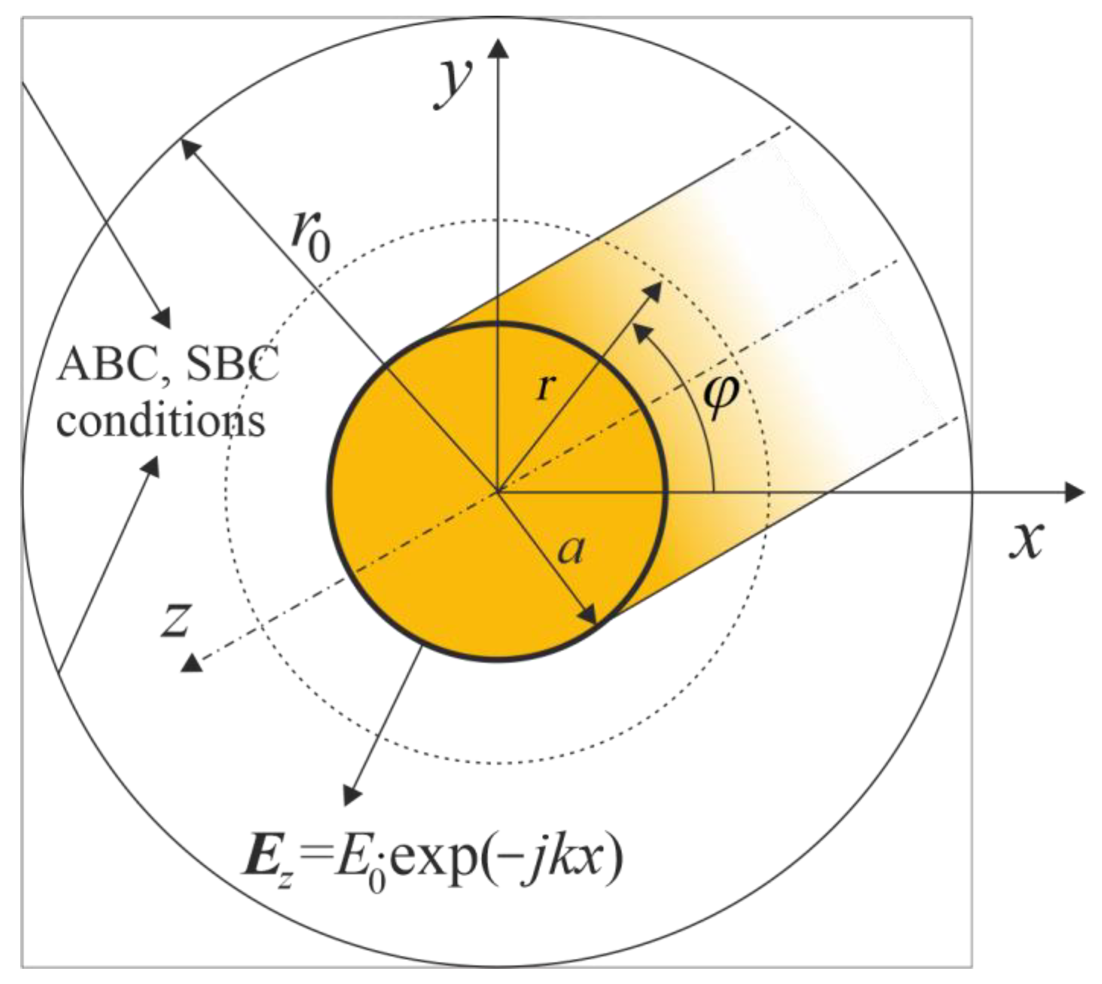
In Figure 1, a plane wave $\underset{¯}{\mathit{E}}=E_0{\mathrm{e}}^{j\left(\omega t-kx\right)}{1}_z$, traveling along the x direction, falls on an infinitely long ideally conducting cylinder of radius a. The expression for the scattered wave is [25]:

$${\underset{¯}{E}}_s=-E_0{\mathrm{e}}^{j\left(\omega t\right)}{\displaystyle \sum _{n=-\infty }^{\infty }{\left(-j\right)}^n}\frac{J_n\left(ka\right)H_n^{\left(2\right)}\left(kr\right){\mathrm{e}}^{jn\phi }}{H_n^{\left(2\right)}\left(ka\right)}$$

(19)

where J_n(·) denotes the Bessel function of the first kind and order n and H_n(·) is the Hankel function of the second kind and order n.

4.1. Results for Circular Boundary

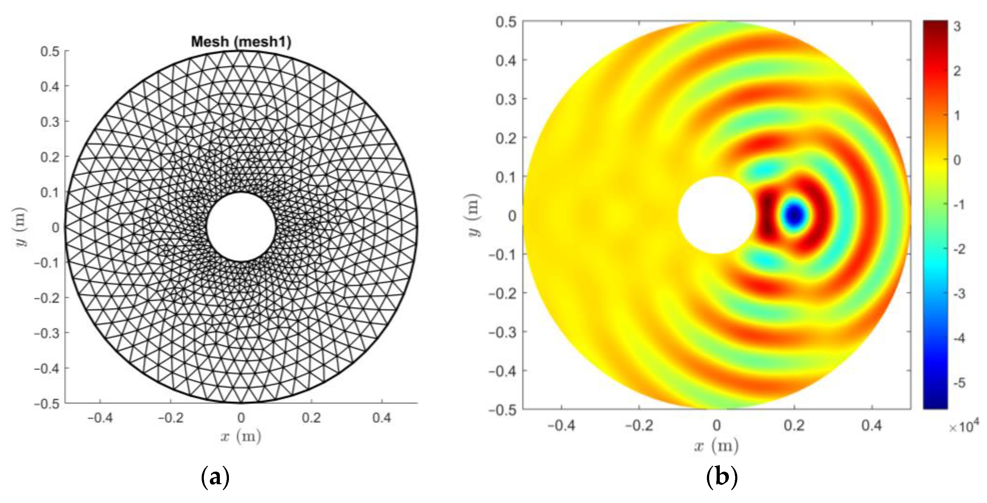
Calculations were carried out for a conducting cylinder of radius a = 0.1 m and artificial circular boundary of radius r₀ = 0.5 m where the SBCs and ABCs were introduced (E₀ = 10 V/m, frequency f = 2.45 GHz). The exemplary finite element mesh is shown in Figure 2a. The mesh used in the FEM calculations was denser and consisted of 24,440 triangular elements. Figure 2b shows the distribution of the real part of the scattered wave E_s using the first-order ABC condition (12). It can be seen that the scattered wave propagates towards the edge of the analyzed area without any distortion.

Additionally, to evaluate the quality of the received results, the normalized root mean square error (NRMSE) was defined as:

$$\mathsf{\in }=\frac{\sqrt{\frac{1}{M}{\displaystyle \sum _{i=1}^M{\left[{\left|E_s\right|}_i^{\left(art\right)}-{\left|E_s\right|}_i^{\left(ana\right)}\right]}^2}}}{\max \left[{\left|E_s\right|}_i^{\left(art\right)}\right]-\min \left[{\left|E_s\right|}_i^{\left(ana\right)}\right]}100\%$$

(20)

where M is the number of evaluated points, ${\left|E_s\right|}_i^{\left(art\right)}$ and ${\left|E_s\right|}_i^{\left(ana\right)}$ denote the absolute value of the electric field vector using SBCs/ABCs imposed on the boundary of radius r₀ and the absolute value of the electric field vector obtained by analytical expression (19), respectively.

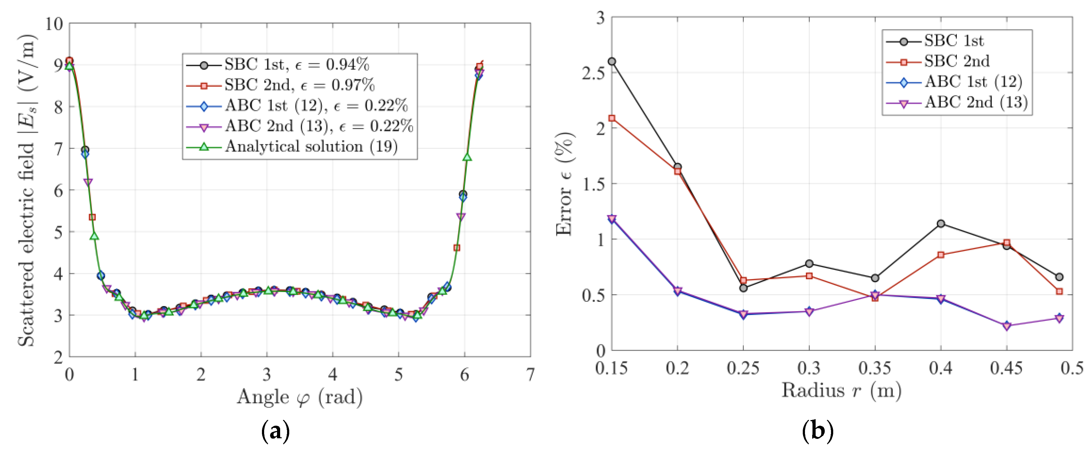
Figure 3a shows the exemplary results obtained for M = 100 equidistant points lying on a virtual circle of radius r. It can be seen that in case of a circular artificial boundary, the derived mathematical expressions give less error ϵ than those existing in COMSOL. Additionally, in Figure 3b, the values of error ϵ for 0 < φ ≤ 2π and different values of radius r are shown. The error values obtained when applying ABCs are also less for the whole range of radius r.

Table 1. Error ϵ (%) values as a function of radius r—Figure 3b.

r (m)	SBC 1st	SBC 2nd	ABC 1st	ABC 2nd
0.15	2.60	2.09	1.18	1.19
0.20	1.65	1.61	0.53	0.54
0.25	0.56	0.63	0.32	0.33
0.30	0.78	0.67	0.35	0.35
0.35	0.65	0.47	0.50	0.50
0.40	1.14	0.86	0.46	0.47
0.45	0.94	0.97	0.22	0.22
0.49	0.66	0.53	0.29	0.29

summarizes the obtained results for a circular boundary (0 < φ ≤ 2π).

4.2. Results for Rectangular Boundary

In this case, the ABCs and SBCs were applied on a square with sides of 1 m (the artificial square boundary is also shown in Figure 1). The mesh used in the FEM calculations consisted of 26,630 triangular elements. All other parameter values and calculation conditions remained the same. The distribution of the real part of the scattered wave E_s using the first-order ABC condition (16) is shown in Figure 4. In this case also, the scattered wave is undistorted.

Figure 5a shows the exemplary calculations obtained for M = 100 equidistant points lying on a virtual circle of radius r. In this situation, the first-order ABC gives a higher error than the SBCs; however, in the case of the second-order ABC, the error ϵ is significantly lower. In Figure 5b, the error ϵ values for 0 < φ ≤ 2π and different values of radius r are shown. The first-order ABC gives the biggest error values; however, in the case of the second-order ABC, the error values are smallest for the entire range of radius r.

The obtained results for the rectangular boundary are summarized in

Table 2. Error ϵ (%) values as a function of radius r—Figure 5b.

r (m)	First-Order SBC	Second-Order SBC	First-Order ABC	Second-Order ABC
0.15	2.03	2.09	6.55	0.04
0.20	1.32	1.95	4.44	0.03
0.25	1.13	1.78	3.87	0.02
0.30	1.55	1.35	4.51	0.02
0.35	1.75	1.91	4.20	0.03
0.40	1.63	1.43	4.72	0.03
0.45	2.57	1.77	6.18	0.05
0.49	2.63	1.12	6.99	0.05

(0 < φ ≤ 2π).

4.3. Results for Mixed Boundaries

In practical applications, it is very important to check the efficiency of the proposed ABCs on mixed boundaries that combine circular and rectangular geometries. Figure 6 presents the distribution of the real part of the scattered wave E_s using the first-order ABCs (12) and (16).

Similarly to previous cases, a detailed comparison was performed. Figure 7a shows the exemplary calculations obtained for M = 100 equidistant points lying on a virtual circle of radius r = 0.28 m. In this situation, the first- and the second-order SBCs give notably higher errors than the ABCs. In Figure 7b, the error ϵ values for 0 < φ ≤ 2π and different values of radius r are shown. In this case, the second- and the first-order ABCs yield the lowest error values for the entire range of radius r.

The obtained results for the rectangular boundary are also summarized in

Table 3. Error ϵ (%) values as a function of radius r—Figure 7b.

r (m)	First-Order SBC	Second-Order SBC	First-Order ABC	Second-Order ABC
0.150	2.49	3.09	0.99	0.96
0.175	1.71	1.97	0.47	0.43
0.200	2.30	2.65	0.57	0.57
0.225	1.44	1.63	0.58	0.53
0.250	1.45	1.98	0.38	0.53
0.275	1.99	2.20	0.54	0.54
0.280	1.85	2.00	0.59	0.57

(0 < φ ≤ 2π).

5. Test Problem 2—Line Source Parallel to Conducting Cylinder

The next type of exterior electromagnetic wave problem where the ABCs can be used is that of an excitation device which sends out waves which do not return. This is termed the radiation problem. As a second test problem, we considered the electromagnetic field excited by a line source, $\underset{¯}{I}=I_0{\mathrm{e}}^{j\omega t}$, parallel to the axis of a conducting cylinder (Figure 8).

In such a case, the total electric field is given by [26]:

$${\underset{¯}{E}}_z=-\frac{\omega {\mu }_0}{2}{I}_0{\displaystyle \sum _{n=0}^{\infty }\frac{1}{1+{\delta }_{0n}}\cos \left(n\left(\phi -{\phi }_0\right)\right)}\left[c_n{H}_n^{\left(2\right)}\left({\beta }_{0}r\right)+J_n\left({\beta }_{0}c\right)H_n^{\left(2\right)}\left({\beta }_{0}r\right)\right]$$

(21)

where ${\underset{\_}{c}}_n=-J_n\left({\beta }_{0}a\right)\frac{H_n^{\left(2\right)}\left({\beta }_{0}c\right)}{H_n^{\left(2\right)}\left({\beta }_{0}a\right)}$, δ_0n denotes the Kronecker delta, ${\beta }_0=\omega \sqrt{{\mu }_0{\epsilon }_0}$, $\left(c,{\phi }_0=0\right)$ and (r, φ) are the coordinates of the points corresponding to the position of the line source and the place of calculation of the total electric field E_z, respectively.

5.1. Results for Circular Boundary

Calculations were also carried out for a perfectly conducting cylinder of radius a = 0.1 m and artificial circular boundary of radius r₀ = 0.5 m where the SBCs and ABCs were introduced (I₀ = 10 A, frequency f = 2.45 GHz). The exemplary finite element mesh is shown in Figure 9a. Figure 9b shows the distribution of the real part of the total electromagnetic wave E_z using the first-order ABC condition (12).

Also, as with the previous test problem, a detailed comparison was performed. Figure 10a shows the exemplary calculations obtained for M = 100 equidistant points lying on a virtual circle of radius r = 0.45 m. In this configuration, the first- and the second-order SBCs and ABCs give similar error values. Analyzing the results in Figure 10b, it can be seen that the errors ϵ obtained by applying the first-order ABC and the SBCs are comparable. However, in the case of the second-order ABC, the obtained error values are definitely lower.

The obtained results for the rectangular boundary are also summarized in

Table 4. Error ϵ (%) values as a function of radius r—Figure 10b.

r (m)	First-Order SBC	Second-Order SBC	First-Order ABC	Second Order ABC
0.25	1.41	0.39	1.37	1.37
0.30	1.37	0.47	1.32	1.33
0.35	1.17	0.65	1.13	1.13
0.40	1.55	0.53	1.49	1.49
0.45	1.29	0.90	0.91	0.91
0.49	1.44	0.64	1.19	1.20

(0 < φ ≤ 2π).

5.2. Results for Rectangular Boundary

In Figure 11a,b, the exemplary calculations are shown. The values of the other parameters are identical to those of the previous calculations. For the current test problem, the ABCs works better than the SBCs implemented in the COMSOL software [23]. The highest error ϵ is obtained for the first-order ABC, for r = 0.5 m, while the second-order ABC performs very well (error ϵ less than 0.5%) for the entire range of radius r.

The obtained results for the rectangular boundary are also summarized in

Table 5. Error ϵ (%) values as a function of radius r—Figure 11b.

r (m)	First-Order SBC	Second-Order SBC	First-Order ABC	Second-Order ABC
0.25	0.60	0.67	0.99	0.11
0.30	1.05	0.66	1.43	0.18
0.35	2.00	0.93	2.17	0.29
0.40	2.27	1.02	3.00	0.30
0.45	3.45	1.13	3.48	0.33
0.49	3.70	0.96	3.65	0.33

(0 < φ ≤ 2π).

5.3. Results for Mixed Boundaries

Similarly, Figure 12a,b show the exemplary results. Generally, the ϵ error values are comparable over the whole range of radius r. However, in the range of r values up to approximately 0.24 m, it appears that the first-order ABC gives smaller error values than the second-order ABC.

The obtained results for mixed circular and rectangular artificial boundaries are also summarized in

Table 6. Error ϵ (%) values as a function of radius r—Figure 12b.

r (m)	First-Order SBC	Second-Order SBC	First-Order ABC	Second-Order ABC
0.225	1.15	0.64	1.14	1.01
0.2311	1.20	0.72	1.20	1.03
0.2372	1.32	0.89	1.27	1.04
0.2433	1.51	1.11	1.39	1.09
0.2494	1.71	1.32	1.55	1.18
0.2556	1.86	1.50	1.68	1.24
0.2617	1.94	1.63	1.75	1.26
0.2678	1.97	1.68	1.77	1.25
0.2739	1.99	1.67	1.77	1.23
0.2800	2.06	1.63	1.82	1.27

(0 < φ ≤ 2π).

In

Table 7. Comparison of degrees of freedom, calculation time, and convergence values.

	First-Order SBC	Second-Order SBC	First-Order ABC	Second-Order ABC
DoF	184,006	186,122	184,006	186,122
Calc. time	2 s	4 s	2 s	4 s
Convergence	1.6·10−14	1.8·10−14	1.1·10−14	1.7·10−14

, the comparisons of degrees of freedom (DoF), convergence, and computational time required for the ABC and the SBC methods used in COMSOL are presented.

6. Conclusions

New, previously unknown (to the best knowledge of the authors of this paper) closed-form expressions for Nth-order ABCs for both two- and three-dimensional electromagnetic scattering problems have been presented. Curiously enough, the coefficients of the Nth-order ABCs are known, for example, as Laguerre, Stirling, and Lah numbers, and arise in many different areas of mathematics and physics. The implementation of the ABCs into the commercial finite element software COMSOL Multiphysics via surface current density boundary conditions is discussed. The obtained results were compared with the scattering boundary conditions existing in COMSOL Multiphysics software and with analytical solutions for two test problems. Generally, for the two test problems analyzed, the second-order ABC gave significantly smaller errors than the SBCs implemented in the COMSOL software. The presented ABCs’ conditions can be implemented and applied to any arbitrarily complex numerical model, but a detailed error comparison is only possible if the exact analytical solution is known.

References

- Han, T.; Han, Y. Numerical solution for super large scale systems. IEEE Access 2013, 1, 537–544. [Google Scholar]
- Gratkowski, S.; Pichon, L.; Razek, A. New infinite elements for a finite element analysis of 2D scattering problems. IEEE Trans. Mag. 1996, 32, 882–885. [Google Scholar] [CrossRef]
- Charles, A.; Towers, M.S.; McCowen, A. A general infinite element for terminating finite element meshes in electromagnetic scattering prediction. IEEE Trans. Mag. 1998, 34, 3367–3370. [Google Scholar] [CrossRef]
- Gratkowski, S.; Ziolkowski, M. On the accuracy of a 3-D infinite element for open boundary electromagnetic field analysis. Archiv. Elektrotech. 1994, 77, 77–83. [Google Scholar] [CrossRef]
- Jin, J.M. The Finite Element Method in Electromagnetics, 3rd ed.; John Wiley & Sons: Hoboken, NJ, USA, 2014. [Google Scholar]
- Mittra, R.; Ramahi, O. Absorbing Boundary Conditions for the Direct Solution of Partial Differential Equations Arising in Electromagnetic Scattering Problems. Prog. Electromagn. Res. 1990, 2, 133–173. [Google Scholar] [CrossRef]
- Gumerov, N.A.; Duraiswami, R. Fast Multipole Methods for the Helmholtz Equation in Three Dimensions; A Volume in Elsevier Series in Electromagnetism; Elsevier: Amsterdam, The Netherlands, 2005. [Google Scholar]
- McDonald, B.H.; Wexler, A. Finite element solution of unbounded field problems. IEEE Trans. Micowave Theory Tech. 1972, 20, 841–847. [Google Scholar] [CrossRef]
- MacCamy, R.; Marin, S. A finite element method for exterior interface problems. Int. J. Math. Math. Sci. 1980, 3, 311–350. [Google Scholar] [CrossRef]
- Jin, J.M.; Riley, D.J. Finite Element Analysis of Antennas and Arrays; John Wiley & Sons, Inc.: Hoboken, NJ, USA, 2009; pp. 55–99. [Google Scholar]
- Bayliss, A.; Turkel, E. Radiation boundary conditions for wave-like equations. Comm. Pure Appl. Math. 1980, 33, 707–725. [Google Scholar] [CrossRef]
- Bayliss, A.; Gunzburger, M.; Turkel, E. Boundary conditions for the numerical solution of elliptic equations in exterior regions. SIAM J. Appl. Math. 1982, 42, 430–451. [Google Scholar] [CrossRef]
- Bayliss, A.; Goldstein, C.I.; Turkel, E. An iterative method for the Helmholtz equation. J. Comput. Phys. 1983, 49, 443–457. [Google Scholar] [CrossRef]
- Medvinsky, M.; Tsynkov, S.; Turkel, E. Direct implementation of high-order BGT absorbing boundary conditions. J. Comput. Phys. 2019, 376, 98–128. [Google Scholar] [CrossRef]
- Gordon, D.; Gordon, R.; Turkel, E. Compact high order schemes with gradient-direction derivatives for absorbing boundary conditions. J. Comput. Phys. 2015, 297, 295–315. [Google Scholar] [CrossRef]
- Zarmi, A.; Turkel, E. A general approach for high order absorbing boundary conditions for the Helmholtz equation. J. Comput. Phys. 2013, 242, 387–404. [Google Scholar] [CrossRef]
- Li, Y.; Cendes, Z.J. High-accuracy absorbing boundary condition. IEEE Trans. Mag. 1995, 31, 1524–1529. [Google Scholar]
- Yao Bi, J.L.; Nicolas, L.; Nicolas, A. Vector absorbing boundary conditions for nodal or mixed finite elements. IEEE Trans. Mag. 1996, 32, 848–853. [Google Scholar] [CrossRef]
- Mur, G. Absorbing boundary conditions for the finite-difference approximation of the time-domain electromagnetic-field equations. IEEE Trans. Electromagn. Compat. 1981, 23, 377–382. [Google Scholar] [CrossRef]
- Sarto, M.S. Innovative absorbing-boundary conditions for the efficient fdtd analysis of lightning-interaction problems. IEEE Trans. Electromagn. Compat. 2001, 43, 368–381. [Google Scholar] [CrossRef]
- Ramahi, O.M. Absorbing boundary conditions for the three-dimensional vector wave equation. IEEE Trans. Antenn. Propag. 1991, 11, 1735–1736. [Google Scholar] [CrossRef]
- Paul, P.; Webb, J.P. Finite element analysis of electromagnetic scattering using p-adaption and an iterative absorbing boundary condition. IEEE Trans. Mag. 2010, 46, 3361–3364. [Google Scholar] [CrossRef]
- COMSOL—Software for Multiphysics Simulation. Available online: http://www.comsol.com (accessed on 30 September 2023).
- Wilcox, C.H. An expansion theorem for electromagnetic fields. Comm. Pure Appl. Math. 1956, 9, 115–134. [Google Scholar] [CrossRef]
- Sadiku, M.N.O. Computational Electromagnetic with Matlab, 4th ed.; Taylor & Francis Group: Boca Raton, FL, USA, 2019; pp. 54–56. [Google Scholar]
- Mrozynski, G.; Stallein, M. Electromagnetic Field Theory; Springer: Cham, Switzerland, 2011; pp. 247–259. [Google Scholar]