Article

Quantitative Assessment of the Impact of Extreme Events on Electricity Consumption
1
School of Earth Sciences, Zhejiang University, 866 Yuhangtang Road, Hangzhou 310027, China
2
Zhejiang Provincial Key Laboratory of Geographic Information Science, 866 Yuhangtang Road, Hangzhou 310027, China
*
Author to whom correspondence should be addressed.
Energies 2024, 17(1), 45; https://doi.org/10.3390/en17010045
Submission received: 31 October 2023 / Revised: 6 December 2023 / Accepted: 19 December 2023 / Published: 21 December 2023
(This article belongs to the Section C: Energy Economics and Policy)

Abstract

:
Global energy consumption is growing rapidly, with the frequency and intensity of extreme events constantly increasing, posing a long-term threat to power supply and consumption. Therefore, analyzing the spatiotemporal characteristics of electricity consumption and quantitatively assessing the impact of extreme events on electricity consumption are of great significance. Based on fine-grained electricity consumption data from Europe for the years 2019–2022, this paper employs a data mining perspective and four methods including Z-score, Isolation Forest, Local Outlier Factor, and Autoencoder to detect abnormal electricity consumption during extreme events. Additionally, it combines indicators such as elastic loss, vulnerability, and duration to measure the impact of extreme events on electricity consumption. It is found that low temperatures could lead to abrupt changes in electricity consumption, with Northern Europe being more significantly affected by low temperatures. The COVID-19 pandemic had the most significant impact on electricity consumption in Europe, with the middle part of Europe being the hardest hit during the first wave of the pandemic. Electricity anomalies during the pandemic period were related to national pandemic control policies and exhibited some lag. High temperatures persisted for a longer duration in the middle part of Europe.

1. Introduction

As the global population grows and the economy develops, the rapid increase in global energy consumption, makes the energy demand and supply issues a focal point of global attention. Electricity, is a significant product of the industrial revolution and an energy resource, which has made substantial contributions to the development and prosperity of modern human society [1]. At the same time, electricity consumption, can be used as a fundamental indicator for measuring the total electricity usage across various sectors and urban and rural residents. The immediacy and sensitivity make it an important index for reflecting economic performance [2,3].
Currently, extreme events have become the norm and are on the rise. Taking recent years as an example, the number of Atlantic hurricanes reached a new high in 2020, with Central America experiencing unprecedented Category 4 hurricanes in November [4]. In the same year, the world faced large impacts from the COVID-19 pandemic [5,6]. In 2021, North America experienced unusual high temperatures, with July becoming the hottest month on record globally, while Europe faced record-breaking rainfall and flooding [7,8]. In the summer of 2022, the Northern Hemisphere was hit by exceptionally high temperatures, with a European heatwave causing over 1000 deaths, multiple countries declaring emergencies, and the UK issuing its first-ever “extreme heat” red warning [9]. The Intergovernmental Panel on Climate Change (IPCC) in its Sixth Assessment Report (AR6) points out that climate change will accelerate in all regions globally in the coming decades, with extreme heat and precipitation events becoming more frequent, and the likelihood of concurrent extreme events increasing, as well [10].
Extreme events pose a serious threat to global electricity supply and consumption, placing them in an unstable state. Extreme events could lead to sharp fluctuations in electricity consumption over short periods, such as a rapid increase in urban electricity usage during heavy rainfall seasons and a significant decrease in electricity demand during drought seasons [11]. Due to the impact of global climate change, the frequency and severity of threat are continually increasing. Countries around the world are increasingly emphasizing the resilience of their power systems, including their ability to resist and recover from extreme events, often measured as “resilience” [12,13,14]. Typically, power system resilience focuses on high-impact, low-probability extreme events [15]. In 2011, the US government released a policy framework for the 21st-century grid, emphasizing the importance of a resilient grid in addressing the impacts of increasingly frequent extreme events. The US National Research Council and the UK House of Lords have also stressed the importance of resilient energy infrastructure [16]. To address extreme events and reduce the losses they cause, it is necessary to quantitatively assess the impact of extreme events on electricity consumption.
Given the current limited quantitative assessment of the impact of extreme events on electricity consumption and the absence of established methods and metrics, this study employs anomaly detection methods to identify electricity consumption patterns in 28 European countries from 2019 to 2022. It combines indicators such as elastic loss, vulnerability, and duration to quantitatively assess the impact of extreme events on electricity consumption.

2. Related Works

As a fundamental and important comprehensive indicator of human life, electricity consumption is influenced by various factors such as the economy, society, geography, and climate. Chen constructed a regression model for global household electricity and fuel consumption. The research results indicate that global household energy consumption is significantly influenced by economic development and population growth. Climate warming will lead to an increase in household electricity consumption, while energy consumption will decrease [17]. Wenz conducted a related study on 35 European countries, and the results indicate that climate change will increase electricity consumption in some countries while decreasing it in certain cities. Extreme weather events will also cause a spatial redistribution of demand from north to south [18]. The COVID-19 pandemic has had profound effects on energy consumption. Buechler E et al. studied the impact of COVID-19 death toll, government strictness index, and individual mobility on global electricity consumption. The results show a close correlation between government restrictions, mobility, holidays, and electricity consumption [19]. Ghiani studied the effects of the COVID-19 outbreak on Italy’s electricity load, consumption, and prices. The results indicate that the pandemic led to a 37% reduction in electricity consumption and a 30% decrease in energy prices [20].
Outlier detection is one of the fundamental tasks in the field of data mining. Outliers may be caused by computational errors or operational mistakes, typically representing non-reproducible errors in normal data [21]. Furthermore, outliers may also result from the inherent variability or elasticity of the data, which holds significant value in practical production and life [22]. Currently, a large number of unsupervised algorithms have been applied to outlier detection. Donovan B, for instance, employed taxi GPS data and used Mahalanobis distance and Z-score for traffic anomaly detection, thereby identifying abnormal time periods affected by hurricanes and conducting resilience analysis [23]. Sun utilized deep autoencoder to detect anomalies in electricity consumption [24]. Li reconstructed input trajectories using autoencoder and performed trajectory anomaly detection by minimizing the difference between the reconstruction output and the original input [25]. In the power grid system, methods like wavelet analysis and autoencoder are often used for anomaly detection to discover potential anomalies in the power grid [26,27].
Theoretical and methodological approaches from resilience assessment were applied to quantitatively assess the resilience of the power system to the shock and impact of extreme events. Examples include the Elasticity Triangle Model [28] and the Elasticity Trapezoid Model [29] for measuring the cumulative disturbances in power consumption. Based upon the Elasticity Trapezoid Model, Tang proposed an elasticity index which considered the spatiotemporal characteristics of extreme events [30]. Reed D. A. characterized the effects of natural disaster events such as hurricanes and earthquakes on network infrastructure by assessing the differences between actual operational states during disaster periods and ideal operational states [31]. In the field of electricity, the focus is primarily on the resilience assessment of the power grid. Zhou calculated the resilience of a distribution network by assessing the degradation area under operational conditions [32]. Li evaluated the resilience of the power grid by combining traditional power system reliability indicators with local topology and topological data analysis methods [33]. However, there have been very few scholars who have conducted quantitative assessments of extreme events on power consumption.
In the analysis of extreme events, it is also common to measure instantaneous disturbances using metrics such as duration and the degree of deviation from normal. Zhang used indicators like vulnerability, robustness, speed, and return level to assess the impact of the COVID-19 pandemic on the subway system [34]. Liu utilized mobile signal data along with metrics like mobile population ratio, daily travel distance, and activity entropy, to measure the impact of the COVID-19 pandemic on population mobility and explored factors influencing population movement [35]. Hong utilized large-scale mobile data to quantify community-level evacuation and recovery patterns in Houston during Hurricane Harvey [36]. Based on the aforementioned research status, this paper quantitatively assesses the impact of extreme events on electricity consumption using metrics such as elasticity loss, duration, and extent of influence.

3. Study Area and Data Sources

3.1. Study Area

Europe is located in the northwest of the Eurasian continent. According to the statistics from the European Union, the total area of Europe is approximately 100,000 square kilometers, with a population of around 749 million at the end of 2022. It comprises 50 independent sovereign countries and is the third most populous continent in the world. In recent years, Europe has become an important region for global electricity consumption, accounting for 20% of the world’s total electricity consumption. However, the European region has been affected by various extreme events such as heatwaves, the Russia-Ukraine conflict, and the COVID-19 pandemic, which have had varying degrees of impact on the electricity market and consumption behavior [20,37,38,39,40,41]. In particular, in 2022, electricity prices in Europe more than doubled, maintaining a leading position in global electricity price increases [42]. Therefore, understanding the dynamic characteristics, behavioral patterns, and influencing factors of the European electricity market and consumption behavior is of significant importance for both theoretical research and practical applications. This paper quantitatively assesses the impact of extreme events on electricity consumption by collecting electricity consumption data from 28 European countries (see Figure 1) for the years 2019–2022.

3.2. Data Sources and Processing

The electricity consumption data in this study are sourced from the European Network of Transmission System Operators for Electricity (ENTSO-E), which provides real-time and historical electricity data. The original data are recorded in Coordinated Universal Time (UTC) with a time resolution of 15 min or 1 h, and are aggregated by country in terms of spatial resolution. However, as electricity consumption data require real-time recording with no gaps, missing data are not acceptable. This study selected 28 countries with data availability exceeding 80% and used forward-filling methods to input missing values in the dataset. To investigate variations in electricity consumption at different scales, this paper aggregates data from hours and minutes into hourly electricity consumption data. These preprocessing steps ensure data reliability and lay the foundation for subsequent research. Data related to the pandemic are sourced from the Our World in Data website, an open online data platform created in collaboration between the University of Oxford and global experts. It provides daily data related to the pandemic from different countries. Meteorological data are obtained from the National Oceanic and Atmospheric Administration (NOAA) in the United States, primarily used to validate the results of extreme event identification. Administrative boundary data are sourced from the Global Administrative Areas Database (GADM). Data sources and detailed processing are shown in Table 1.

4. Research Methods

4.1. Anomaly Detection Methods

Anomaly detection is the process of identifying data points that are significantly different from the rest of the data within a dataset. In this paper, common anomaly detection methods, including Z-score, Isolation Forests, Local Outlier Factors, and Autoencoder, were employed for anomaly detection. These methods were then combined with anomaly duration to identify extreme events. The impact of extreme events on the power system was quantitatively assessed using metrics such as elastic loss and vulnerability.

4.1.1. Z-Score

Z-score anomaly detection is a commonly used statistical method. Its basic idea is to compare each data point with the mean of the dataset and then calculate its standard deviation, resulting in a Z-score. If the Z-score exceeds a certain threshold, the data point can be considered an outlier. The formula to calculate the Z-score is as follows:
Z = ( X μ ) σ
In this equation, X represents the hourly electricity consumption, μ is the mean of the dataset, and σ is the standard deviation of the dataset. Considering the strong periodicity of electricity consumption, this paper simultaneously considers the division of electricity consumption data based on both the day of the week and the hour to calculate their respective means and standard deviations.

4.1.2. Isolation Forest

Isolation Forest (IF) is an anomaly detection algorithm based on a tree structure. Its basic idea is to leverage the splitting capability of random trees to randomly partition data points into different branches. Subsequently, it determines whether a data point is an outlier by calculating its depth in the tree. Normal values have a greater depth in the tree, while outliers have a smaller depth. The calculation process of the Isolation Forest is as follows:
s ( x ) = 2 E ( h ( x ) ) c ( n )
where E(h(x)) represents the expected value of the average path length of sample point x across all trees. c(n) is a constant that can be approximated as:
c ( n ) = 2 H n 1 2 ( n 1 ) n
where H n 1 is the harmonic number, defined as:
H ( n 1 ) = I n ( n ) + 0.5772156649
where I n ( n ) is the natural logarithm base e. Through calculation, the isolation forest score for a sample point could be obtained. The score ranges from 0 to 1, with lower scores indicating that the sample point is more likely to be an outlier. In practical applications, normal points may be labeled as 1, while outliers are labeled as −1.

4.1.3. Local Outlier Factor

The Local Outlier Factor (LOF) is a density-based outlier detection algorithm that identifies outliers based on the density information of sample points. Its calculation process is as follows:
(1) For each data point, find its k-nearest neighbors (kNNs).
(2) Calculate the reachability distance for each data point, which is defined as the distance to the furthest point in its kNN, using the reachability distance formula:
r e a c h d i s t k ( x , y ) = max { d i s t k ( x , y ) , k d i s t k ( y ) }
where d i s t k ( x , y ) represents the distance between x and y at the k-th distance, where the k-th distance indicates the distance to the point that is the k-th closest to x.
(3) Calculate the local reachability density (LRD) for each data point within the kNN space, which is the reciprocal of the average reachability distance to all points in its kNN. The LRD formula is as follows:
L R D K ( x ) = 1 / y N k ( x ) r e a c h d i s t k ( x , y ) N k ( x )
where k is the number of nearest neighbors, and N k ( x ) represents the set of k-nearest neighbors for point x.
(4) Calculate the LOF value for each data point, which represents the ratio of the density of the point relative to its neighborhood to the average density of the surrounding data points. The LOF formula is as follows:
L O F K ( X ) = y N k ( x ) L R D K ( y ) L R D K ( x ) N k ( x )
(5) Based on the computed results, data points with higher LOF values are considered outliers. In practical applications, normal points are assigned a label of 1, while outliers are assigned a label of −1.

4.1.4. Autoencoder

Autoencoder (AE) is an unsupervised learning method that primarily comprises two parts: an encoder and a decoder. The encoder projects input data into a hidden space, while the decoder reconstructs vectors from the hidden space back into the original data. An autoencoder can calculate the error between the original data and the reconstructed data, and if the error exceeds a threshold, the data are considered an anomaly. The implementation process of an autoencoder is as follows:
For a given training set X = {x1, x2, …, xm}, the encoder maps X to a hidden layer, producing encoder output H = {h1, h2, …, hm} as follows:
H = g ( W 1 X + b 1 )
Here, W1 is the weight matrix, b1 is the bias vector.
Then, the hidden layer H is decoded by the decoder into a vector Z = {z1, z2, …, zm} back into the original data distribution as follows:
Z = g ( W 2 H + b 2 )
Here, W2 is the weight matrix and b2 is the bias vector.
Finally, the reconstruction error is calculated, and the backpropagation algorithm is used to optimize the network’s parameters (W1, W2, b1, b2) to minimize the error.

4.2. Extreme Event Detection

Extreme events can lead to changes in electricity consumption by affecting human behavior. This paper combines two parameters, anomaly threshold and time threshold, for the recognition of extreme events, as expressed by the following formula:
E v e n t = { s i : s i | θ | a n d ( T i T j ) t }
Here, E v e n t represents the recognized extreme events, s indicates the anomaly score, and an event is recognized when the value of s exceeds the specified anomaly threshold θ . T i represents the time when an anomaly is recognized, T j represents the time when the next anomaly is recognized, and if the time difference between them exceeds the time threshold t , it indicates the end of this extreme event.
The anomaly threshold varies for different anomaly detection methods. This study establishes the abnormal proportion at 5% based on statistical analysis. For Z-score, it is set at 1.96, indicating that the proportion of anomalies is less than or equal to 5%. For the Isolation Forest (IF) method, 100 trees are used, and the anomaly proportion is set to 5%. In the case of the Local Outlier Factor (LOF) model, the number of local neighbors is set to 24, and the anomaly proportion is also set to 5%. As for the Autoencoder (AE) method, the anomaly proportion is set to 5%. The time threshold t can be chosen based on specific requirements. In this study, to examine the impact of events such as low temperature, high temperature, and epidemics, considering their relatively long durations, the time threshold is set to 168 h, which is equivalent to one week. If no anomalies occur within one week, the event is considered to have ended.

4.3. Quantitative Assessment of Extreme Events

Once extreme events are identified, it is possible to quantitatively assess the perturbations in electricity consumption caused by these extreme events. This paper utilizes three quantitative measures, elastic loss (TLR), vulnerability (V), and duration (T), to evaluate the extent of electricity consumption’s response to extreme events. Duration is defined as the time it takes for the system to reach a new equilibrium state from the beginning of the impact, i.e., from t0 to t1.
The formula for calculating elastic loss (TLR) is as follows:
T L R = t 0 t 1 | 1 Q ( t ) | d t
where TLR represents the elastic loss, reflecting the cumulative disturbance of extreme events on electricity consumption. Q(t) represents the ratio of actual electricity consumption at time t to the average electricity consumption during that period, t0 is the start time of the detected extreme event, and t1 is the end time of the detected extreme event.
The formula for calculating vulnerability (V) is as follows:
V = | E ¯ t E t E ¯ t |
where V represents vulnerability, reflecting the instantaneous disturbance of extreme events on electricity consumption. E ¯ t represents the average electricity consumption at time t and E t is the actual electricity consumption at time t.

5. Result

5.1. Electricity Consumption Anomaly Detection

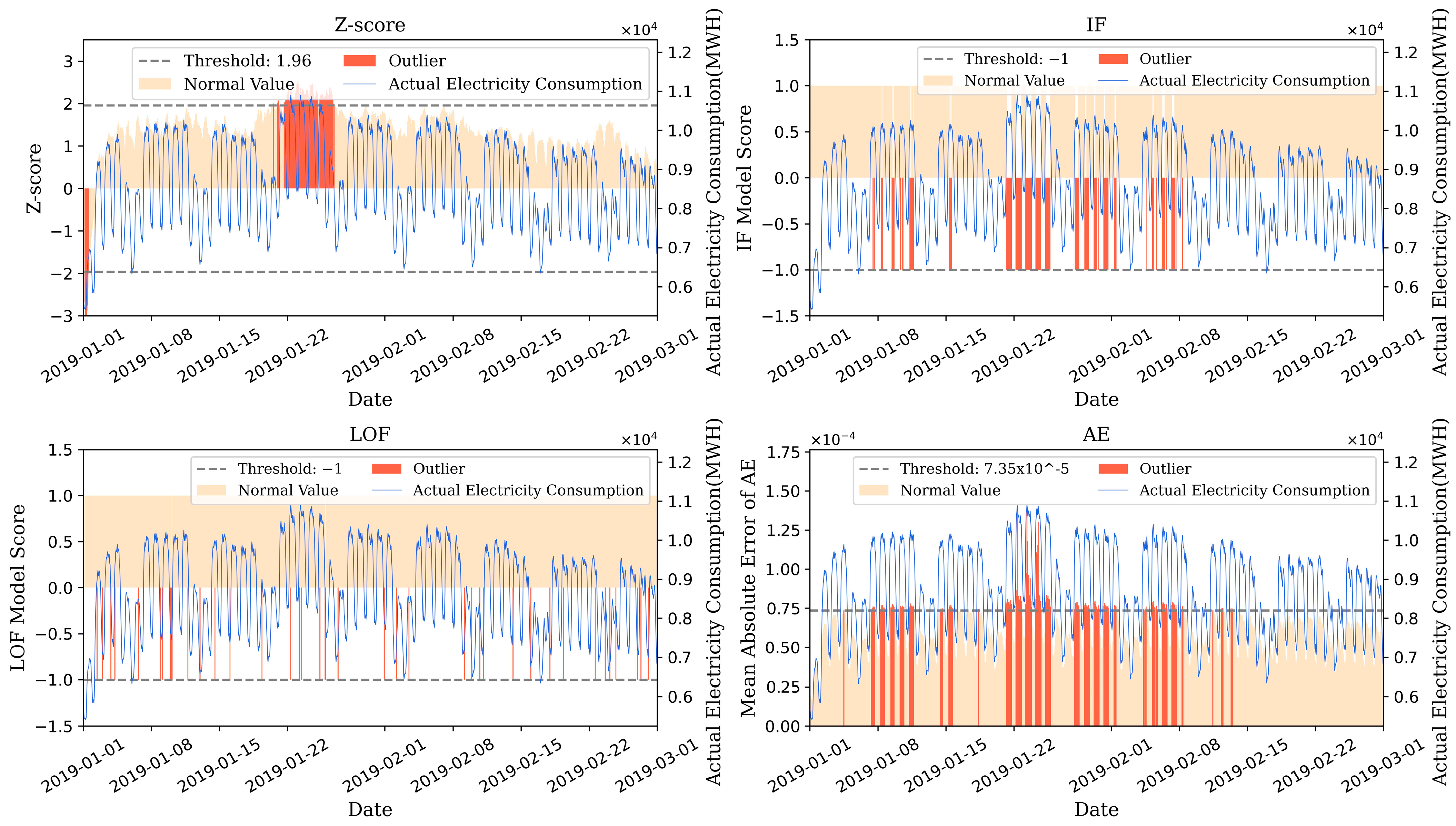
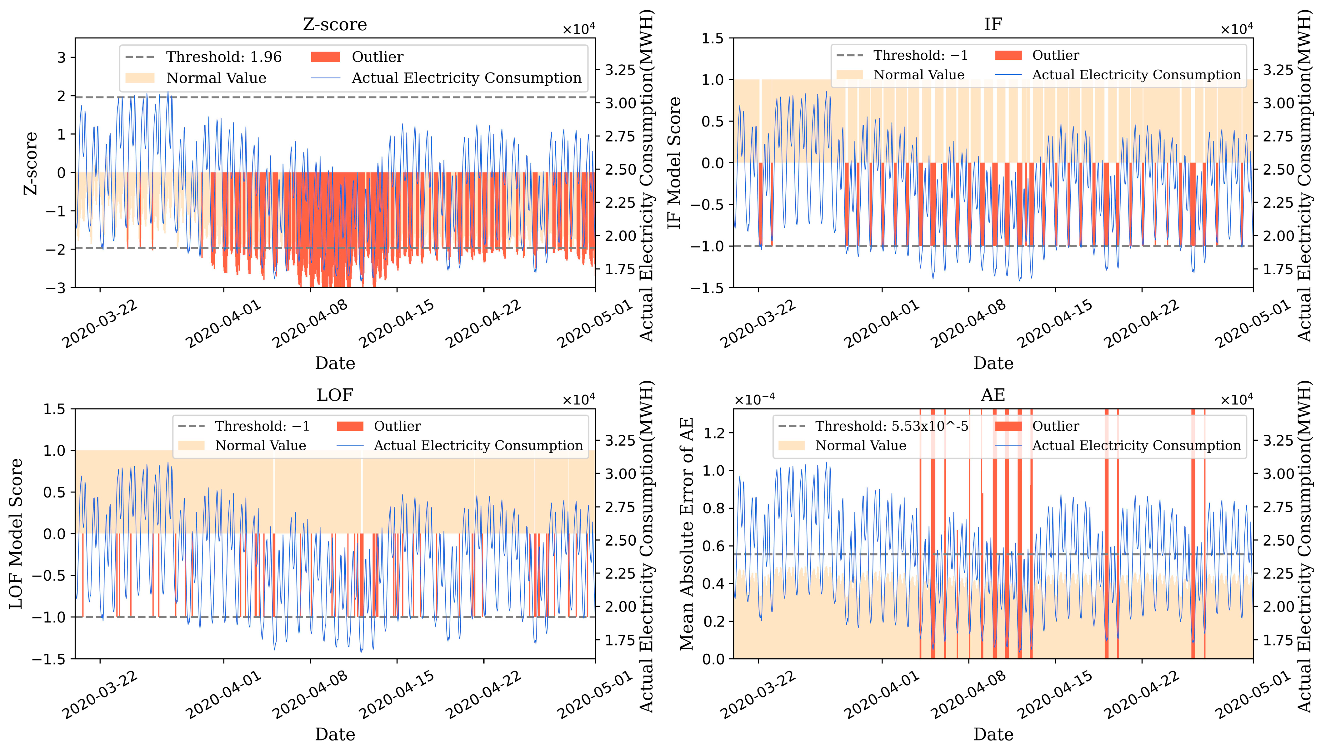
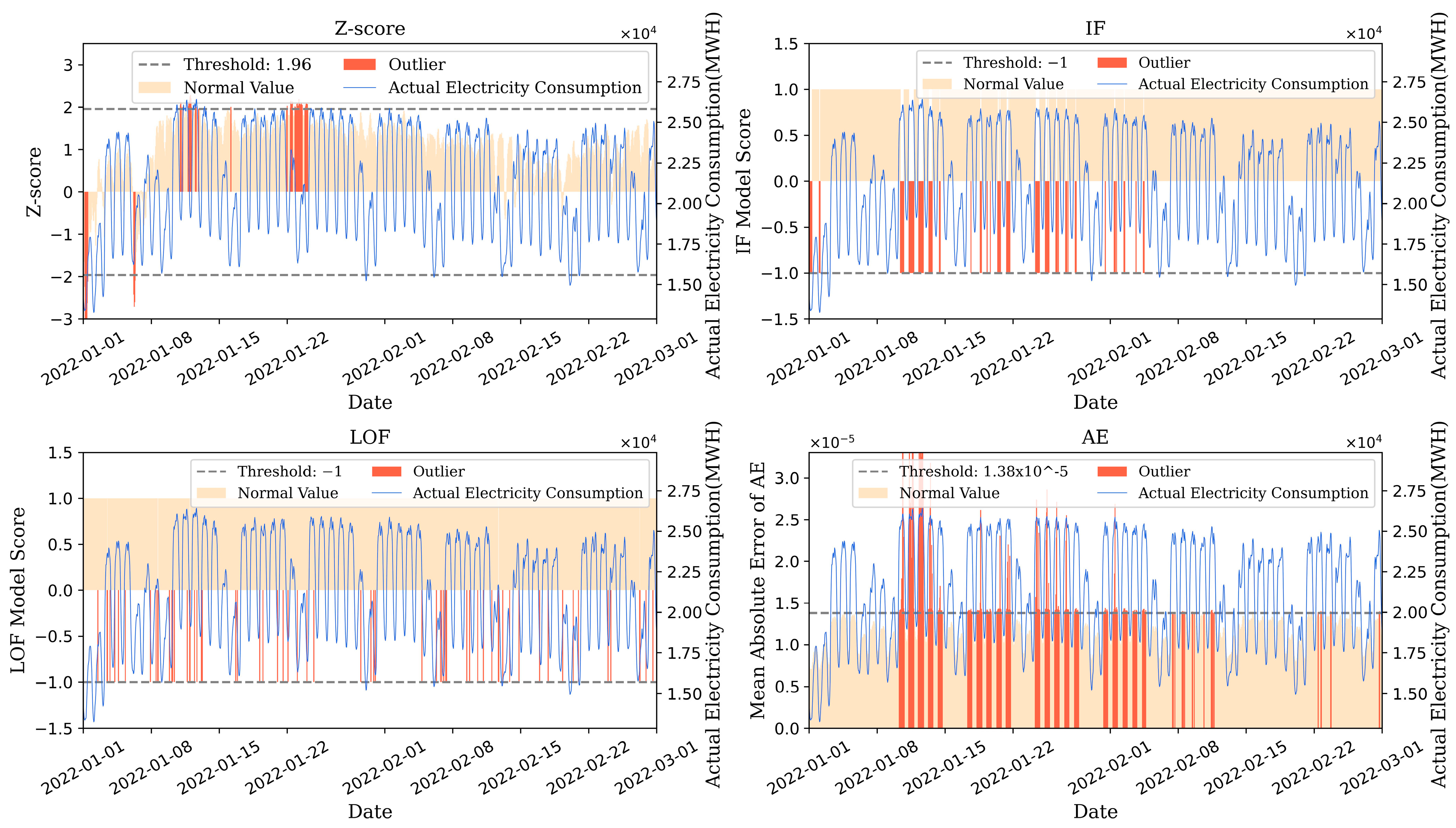
Anomaly detection can help quickly identify and process abnormal electricity usage data, thereby pinpointing the times when extreme events impact power consumption. During late January to early February 2019, multiple European countries experienced the impact of snowstorms and low temperatures. Subsequently, in February 2020, a pandemic broke out in Europe. Concurrently, since January 2022, tensions between Russia and Ukraine have been escalating. Therefore, this article presents selected test results from some countries during the periods from 1 January to 1 March 2019, from 20 March to 1 May 2020, and from 1 January to 1 March 2022. In the accompanying graphs, the blue curve represents actual electricity usage, while the bar chart represents model scores, with the orange bars indicating normal values and the red bars indicating identified anomalies. According to Figure 2, the LOF method seems to be not suitable for anomaly detection in the Czech region, as the anomalies it detects are uniformly distributed. Specifically, the Z-score method can only identify significant increases in electricity consumption during the period from 20 January to 26 January. In contrast, the Isolation Forest (IF) and Autoencoder (AE) methods identify more abnormal time periods, including from 7 January to 11 January and from 28 January to 1 February. In the case of electricity consumption detection in Spain (see Figure 3), the IF method first identifies an anomaly occurring at 2:00 a.m. on 22 March. The IF method and Z-score method both successfully detect abnormal time periods, while the AE method can only identify significant decreases in electricity consumption. The results of anomaly detection in Poland, as one of the countries closest to Ukraine, are illustrated in Figure 4, indicating that the IF and Z-score methods can promptly identify anomalies.
In summary, the LOF method performs poorly in detecting anomalies and cannot effectively distinguish between normal and abnormal values. This may be due to the fact that the outlier points in the electricity consumption dataset exhibit certain time series characteristics, making it difficult for the LOF algorithm to capture these outlier points. The Z-score model can only identify time periods with the most noticeable changes in electricity consumption. The AE method has lower sensitivity for countries with large fluctuations in electricity consumption. In contrast, the IF model performs relatively consistently in various situations and can accurately detect anomalies.

5.2. Extreme Event Recognition

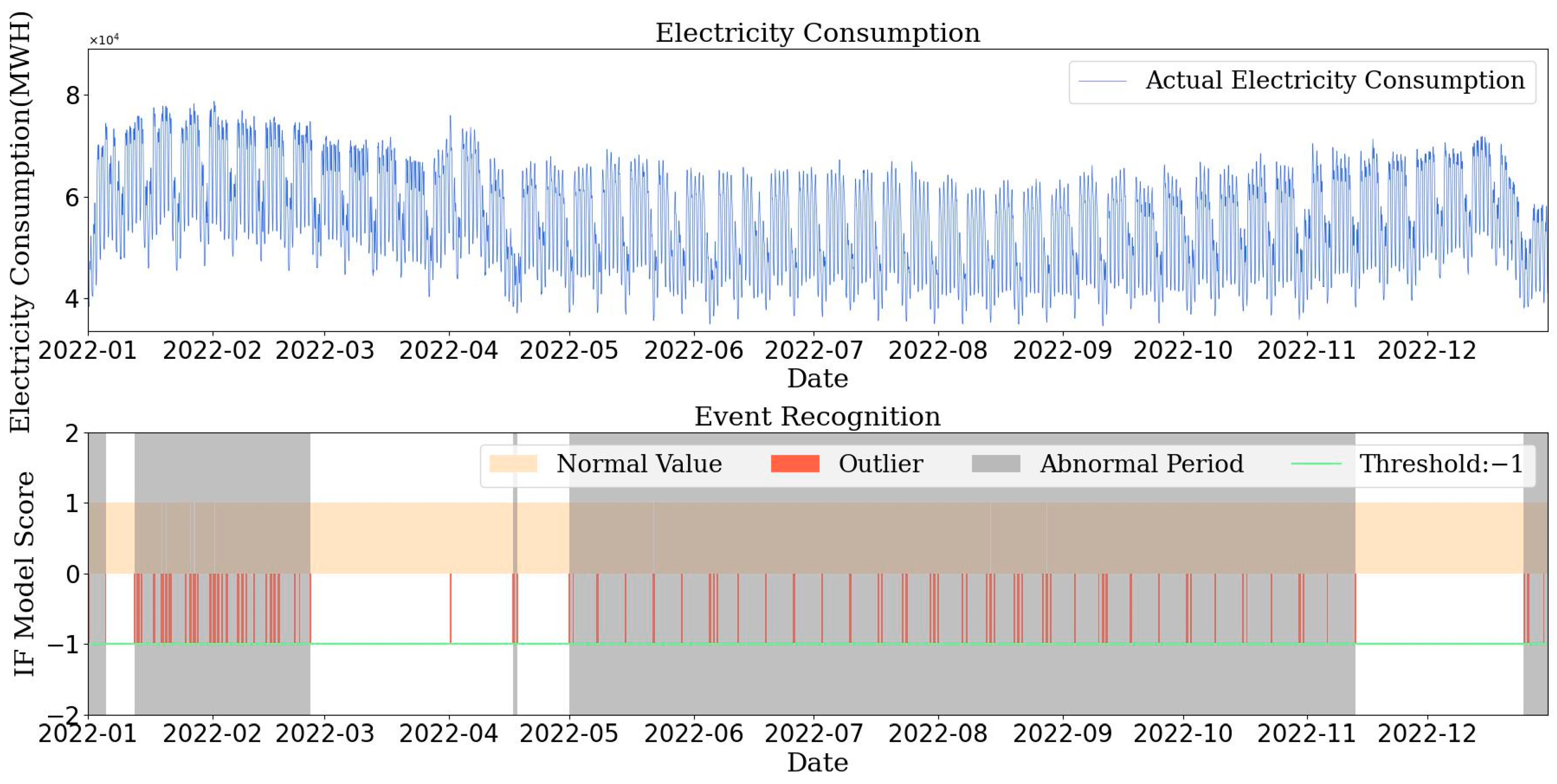
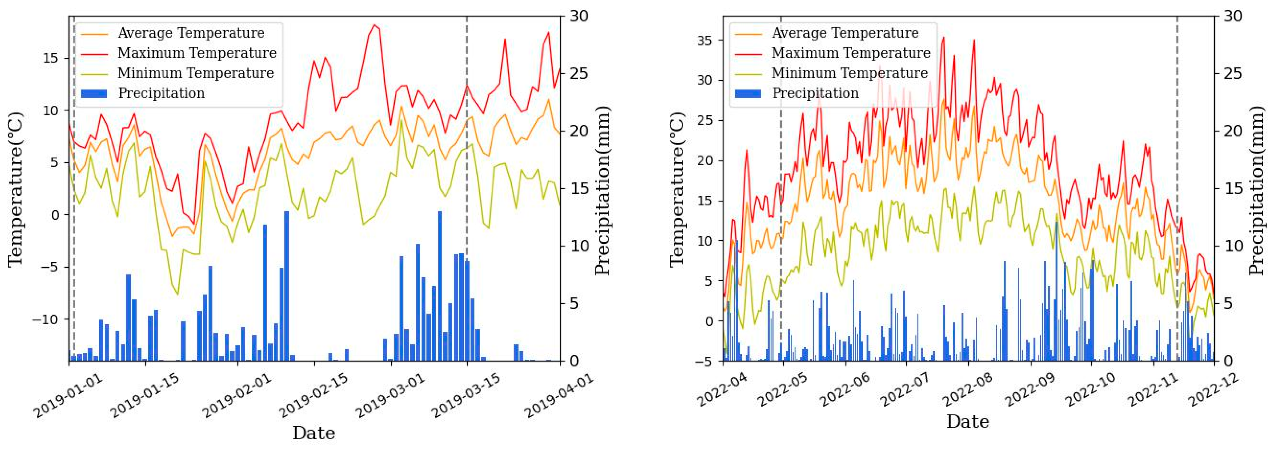
This study aims to analyze the impact of the low temperatures in Europe in 2019, the pandemic in 2020, and the high-temperature events in 2022 on electricity consumption, utilizing data from the respective years for in-depth research. Figure 5 and Figure 6 respectively depict the anomaly detection results for the Netherlands in 2019 and Germany in 2022. The anomaly period for the Netherlands spans from 2 January 2019, at 16:00 to 15 March 2019, at 9:00, totaling 71 days. Considering the meteorological distribution in the Netherlands (Figure 7), this timeframe coincides with the lowest recorded temperatures in the Netherlands. Additionally, starting from 10 March 2019, temperatures in the Netherlands steadily increased until reaching their peak on 15 March, when electricity consumption returned to normal.
For Germany, the anomalous period during the summer of 2022 ranges from 30 April 2022, at 23:00 to 13 November 2022, at 4:00. Examining the temperature variations in Germany, it can be observed that temperatures began to rise at the end of April, started to decline in September, experienced a brief increase in October, and then resumed a decline in November. Around 13 November, a slight temperature drop occurred, coinciding with the return to normal electricity consumption. In conclusion, the results of extreme event identification can be utilized to detect extreme weather events.
Figure 8 displays the results of identifying the COVID-19 pandemic in Italy in 2020. The anomaly period spans from 15 March 2020, at 1:00 to 21 June 2020, at 4:00. The onset of the anomaly occurred approximately two weeks after Italy implemented strict lockdown measures, while the end of the anomaly period coincided with a week after the reduction in lockdown levels. This indicates that the model’s detection results align with the timing of the pandemic and can be used to characterize the pandemic event.

5.3. The Impact of Extreme Events on Electricity Consumption

In the previous section, we used the Isolation Forest (IF) model to identify the impact periods of extreme events on electricity consumption. In this section, we will use duration, elastic loss, and vulnerability indicators to quantitatively assess the impact of extreme events.
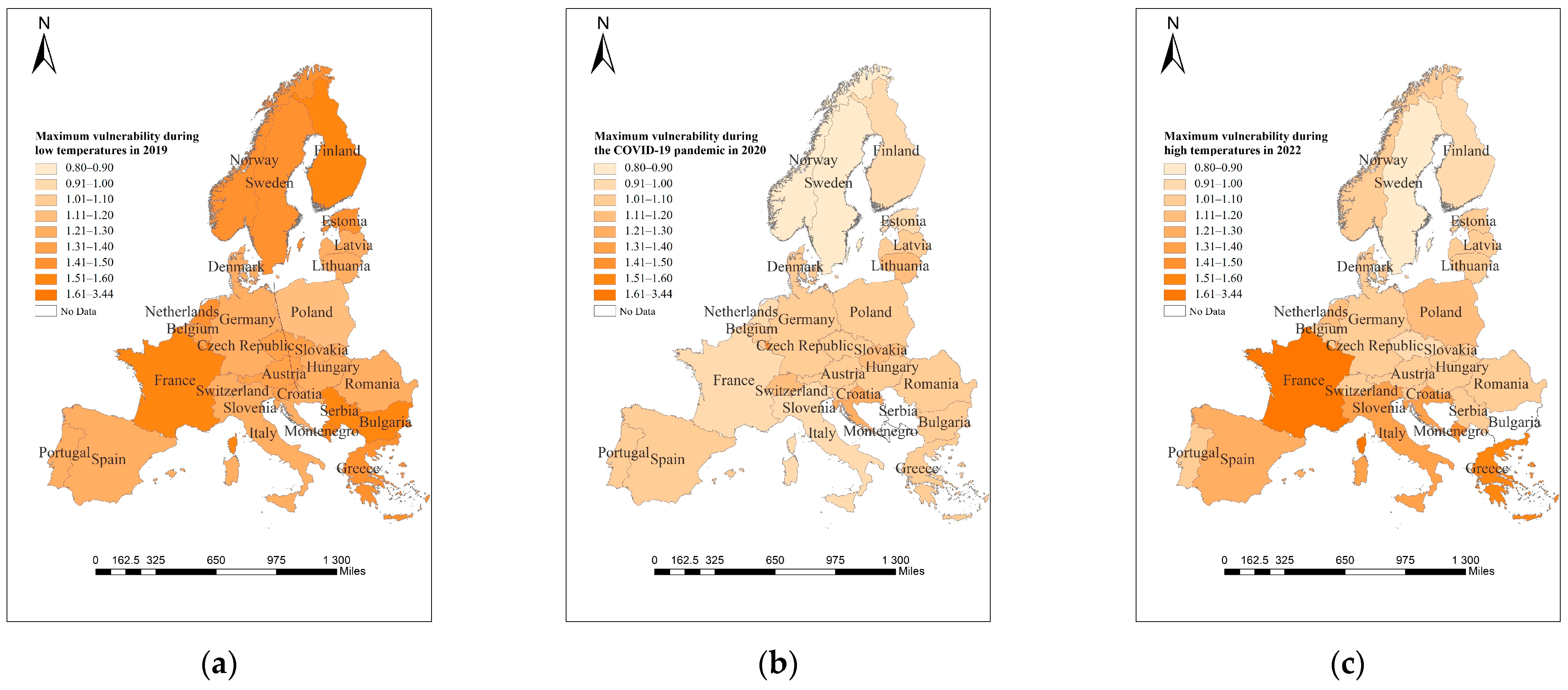
The spatial distribution map of maximum vulnerability is shown in Figure 9. From Figure 9a, it can be seen that the values of maximum vulnerability in Northern Europe and Southern Europe are much higher than in other regions. This indicates that the impact of low temperatures on Northern and Southern Europe is much greater than in other regions. Compared to other extreme events, the maximum vulnerability to low temperatures is much higher, suggesting that low temperatures are more likely to cause a sharp change in electricity consumption. During the pandemic period (Figure 9b), except for Serbia, there is no significant difference in the maximum vulnerability of other countries, indicating that the pandemic has had a significant impact on electricity consumption across the entire European region. During the 2022 heat event, the maximum vulnerability gradually decreases from south to north, indicating that the change in electricity consumption is higher in southern Europe than in the north, and northern Europe is less affected by this event.
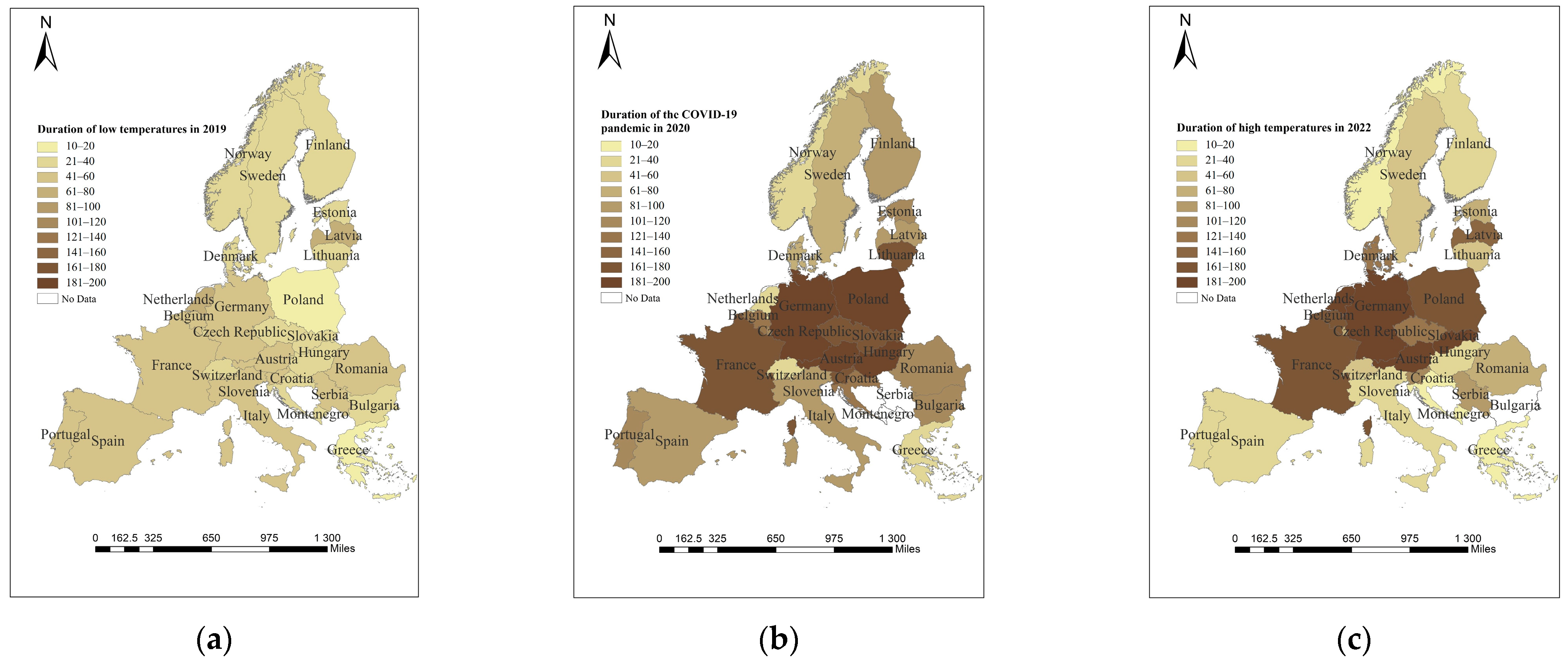
The distribution chart of the duration of extreme events (Figure 10) reveals that the impact of the COVID-19 pandemic on Europe persists longer than other extreme events. In the central part of Europe, electricity consumption experiences an unusually extended duration of impact compared to other regions, indicating that the middle part of Europe was the primary region affected by the first wave of the pandemic. Low temperatures have a shorter duration across the nation and exhibit a relatively even distribution, with slightly longer durations in the southern regions, possibly due to the influence of cold air moving southward. High temperatures show a longer duration in the central part of Europe, which may be related to the climatic zone and topographical features of the middle part of Europe.
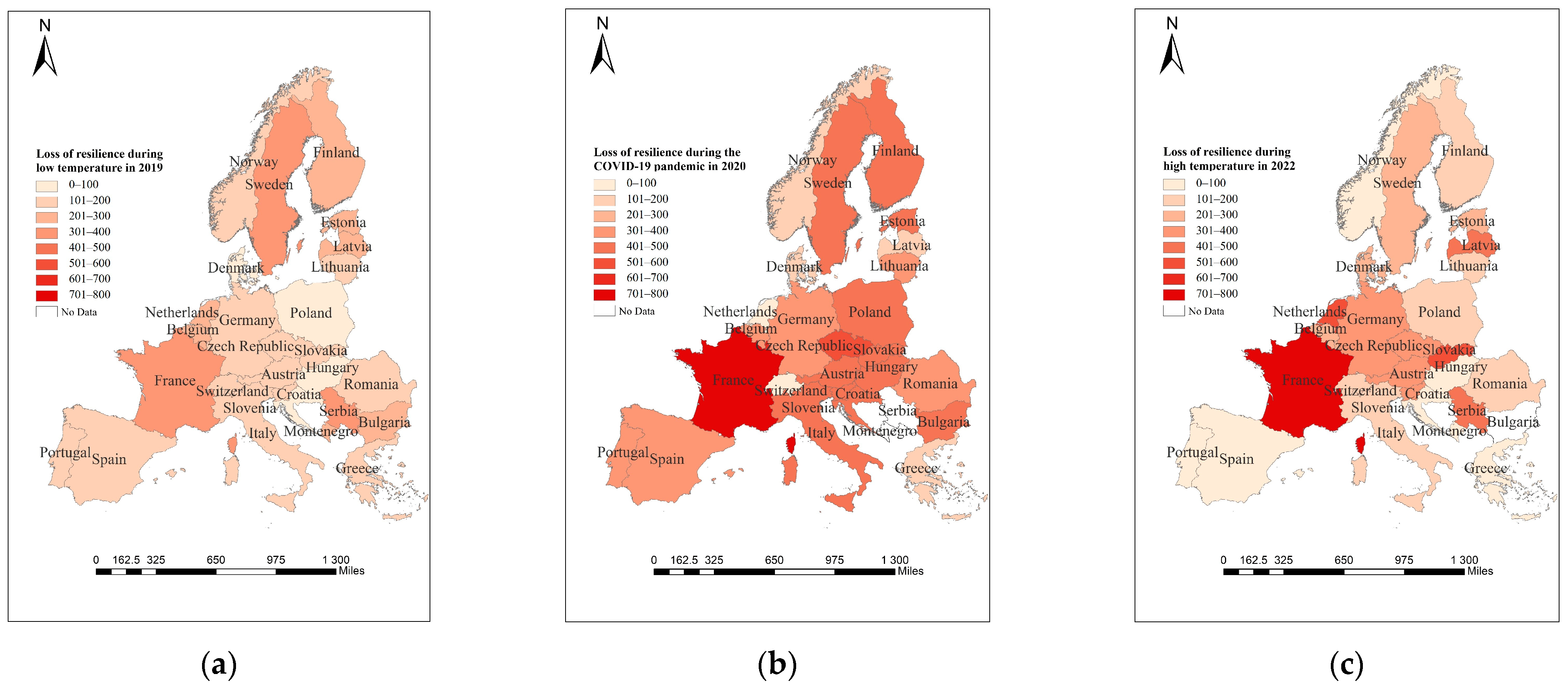
The distribution of elastic losses, as shown in Figure 11, indicates that the elastic losses resulting from the COVID-19 pandemic are higher than those from the other two events. This could be attributed to the prolonged duration of the pandemic. Among the countries, France stands out with the most significant losses caused by the pandemic, while the least affected countries, apart from Montenegro and Serbia, are Switzerland and the Netherlands. It is worth noting that both Montenegro and Switzerland did not implement complete lockdown measures during the pandemic. High temperatures resulted in electricity losses that are second only to those caused by the pandemic, with a greater impact on the central region of Europe compared to other areas. France experienced the most substantial losses due to high temperatures. Low temperatures caused lower electricity losses across Europe compared to the other two events. Among countries, France, Sweden, and Serbia exhibit more noticeable elastic losses due to low temperatures. In summary, it is evident from the comparison that Sweden, France, and Serbia are more sensitive to extreme events in terms of electricity consumption. Under all three extreme events, their elastic losses are higher than in other countries.
Figure 11. Spatial distribution map of elastic loss. (a) The low temperature event in 2020; (b) The COVID-19 pandemic in 2020; (c) The high temperature event in 2022.The disturbance results for electricity consumption under low temperatures, high temperatures, and the COVID-19 pandemic are presented in Table 2, Table 3 and Table 4. From Table 2, it can be observed that the onset of low temperatures is generally in early January, with Norway being the latest to experience temperature drops, starting from 12 January 2019. However, electricity consumption disruptions in Norway did not commence until 14 January, resulting in a delay of 2 days. This highlights the resilience of electricity consumption to extreme events. In comparison to other countries, Norway experienced disturbances later, possibly due to the fact that it already relies on a substantial amount of heating equipment during its cold winter seasons, indicating that electricity consumption in cold regions exhibits better stability under low-temperature conditions.
Energies 17 00045 g011
Table 2. Impact of low temperatures on electricity consumption.
CountryStart TimeEnd TimeDuration
(Days)
Elastic
Loss
Maximum
Vulnerability
Austria7 January 2019 8:0022 February 2019 10:0046192.571.31
Belgium3 January 2019 16:001 March 2019 10:0056204.161.33
Bulgaria2 January 2019 16:0029 January 2019 17:0027208.601.51
Croatia3 January 2019 16:0031 January 2019 18:002886.611.25
Czech Republic7 January 2019 12:008 February 2019 8:0031149.731.32
Denmark3 January 2019 16:007 February 2019 17:003578.541.21
Estonia3 January 2019 14:0013 February 2019 7:0040238.641.46
Finland2 January 2019 10:007 February 2019 17:0036288.031.55
France3 January 2019 7:0015 February 2019 7:0043385.281.57
Germany1 January 2019 3:0019 February 2019 17:0049142.471.26
Greece3 January 2019 8:0022 January 2019 18:0019112.751.43
Hungary1 January 2019 2:0025 January 2019 16:002471.091.26
Italy1 January 2019 3:0014 February 2019 17:0044120.271.22
Latvia3 January 2019 8:0012 March 2019 8:0068220.551.29
Lithuania4 January 2019 15:004 February 2019 9:0030107.371.26
Luxembourg6 January 2019 18:0029 January 2019 7:0022110.641.65
Montenegro3 January 2019 16:001 February 2019 16:0029203.181.58
Netherlands2 January 2019 16:0015 March 2019 9:0071267.621.41
Norway14 January 2019 6:007 February 2019 16:0024192.941.45
Poland1 January 2019 2:0011 January 2019 16:001028.401.16
Portugal1 January 2019 5:0020 February 2019 19:0050158.231.29
Romania7 January 2019 15:0028 February 2019 17:0052193.461.27
Serbia3 January 2019 9:0014 February 2019 18:0042347.891.59
Slovakia7 January 2019 8:0013 February 2019 11:0037146.841.25
Slovenia1 January 2019 2:0025 February 2019 12:0055193.461.37
Spain1 January 2019 3:0019 February 2019 19:0049159.001.27
Sweden2 January 2019 16:0012 February 2019 7:0040308.651.47
Switzerland7 January 2019 11:0013 February 2019 9:0036154.491.30
Table 3. Impact of high temperatures on electricity consumption.
CountryStart TimeEnd TimeDuration
(Days)
Elastic
Loss
Maximum
Vulnerability
Austria1 May 2022 1:001 November 2022 3:00184376.831.07
Belgium29 May 2022 3:0013 November 2022 3:00168287.001.06
Bulgaria18 July 2022 11:004 August 2022 11:001762.381.37
Croatia8 May 2022 0:0018 September 2022 4:00133386.050.99
Czech Republic15 May 2022 2:0025 September 2022 3:00133297.811.08
Denmark5 June 2022 1:0021 August 2022 3:0077280.111.08
Estonia24 June 2022 0:002 August 2022 1:0039165.610.91
Finland8 May 2022 2:001 November 2022 5:00177714.523.44
France30 April 2022 23:0013 November 2022 4:00196356.291.07
Germany16 July 2022 10:002 August 2022 11:001796.061.54
Greece31 July 2022 0:0022 August 2022 2:002249.251.02
Hungary21 June 2022 8:0029 July 2022 15:0038162.211.35
Italy28 May 2022 1:0018 October 2022 0:00142424.281.05
Latvia7 May 2022 22:0026 June 2022 2:0049129.021.04
Lithuania3 June 2022 10:004 August 2022 10:0062291.861.38
Luxembourg22 July 2022 11:0010 August 2022 12:001981.591.42
Montenegro9 April 2022 12:0018 October 2022 12:00192596.811.11
Netherlands20 July 2022 1:0031 July 2022 4:001160.961.08
Norway1 May 2022 3:0016 October 2022 2:00167176.181.11
Poland14 August 2022 2:004 September 2022 4:002134.801.02
Portugal23 April 2022 23:0027 June 2022 0:0064158.761.01
Romania24 April 2022 3:0019 July 2022 1:0085402.371.04
Serbia15 May 2022 1:0013 November 2022 3:00182505.971.01
Slovakia10 July 2022 1:006 November 2022 4:00119351.501.08
Slovenia12 July 2022 11:002 August 2022 12:002153.841.22
Spain24 June 2022 0:0014 August 2022 3:0051280.040.88
Sweden2 July 2022 21:0028 August 2022 11:0056145.081.09
Table 4. Impact of COVID-19 pandemic on electricity consumption.
CountryStart TimeEnd TimeDuration
(Days)
Elastic
Loss
Maximum
Vulnerability
Austria5 April 2020 1:0011 October 2020 2:00189488.351.09
Belgium3 April 2020 1:003 August 2020 2:00122311.751.02
Bulgaria16 April 2020 23:0027 July 2020 1:00101416.381.00
Croatia22 March 2020 1:0031 July 2020 13:00131433.011.22
Czech Republic10 April 2020 22:0027 September 2020 3:00169517.431.04
Denmark23 May 2020 2:009 August 2020 3:0078191.301.03
Estonia24 May 2020 0:002 September 2020 0:00101456.080.94
Finland24 May 2020 1:0024 August 2020 0:0091423.420.92
France11 April 2020 2:0021 September 2020 2:00163740.440.95
Germany5 April 2020 0:004 October 2020 3:00182386.131.07
Greece5 April 2020 2:0013 May 2020 0:0037189.141.07
Hungary29 March 2020 2:005 October 2020 1:00189430.181.08
Italy15 March 2020 1:0021 June 2020 4:0098449.700.99
Latvia17 May 2020 1:009 August 2020 3:0084186.411.05
Lithuania5 April 2020 23:0014 September 2020 0:00161382.901.12
Luxembourg3 August 2020 15:0028 November 2020 16:00117637.571.49
Montenegro4 April 2020 11:0027 April 2020 13:002364.160.99
Netherlands13 June 2020 0:006 July 2020 1:0023129.620.82
Norway29 March 2020 1:004 October 2020 2:00189428.011.07
Poland22 March 2020 4:005 July 2020 6:00105330.731.01
Portugal12 April 2020 0:002 August 2020 3:00112318.731.09
Romania9 April 2020 23:005 October 2020 1:00178450.461.19
Serbia11 April 2020 0:004 October 2020 1:00176463.391.09
Slovakia22 March 2020 2:0021 June 2020 5:0091308.311.04
Slovenia13 June 2020 2:0023 August 2020 4:0071402.120.89
Spain9 April 2020 3:009 May 2020 23:003092.261.12
The Netherlands and Latvia were impacted by low temperatures for the longest duration. In the case of the Netherlands, the temperature began to drop from 1 January 2019, and abnormal electricity usage was identified on 2 January, causing a 1-day delay in electricity disruption. The disturbance in electricity consumption in the Netherlands ended on 15 March. Prior to this date, the temperature in the Netherlands gradually rose from 10 March, reaching its maximum value by 15 March, and electricity consumption also gradually returned to normal. This suggests that the Dutch power system was able to respond promptly to the temperature increase. The prolonged duration of electricity disruption in the Netherlands may be attributed to significant temperature fluctuations during that period, including multiple instances of sudden temperature drops and other extreme weather changes. Latvia also experienced several instances of temperature fluctuations between 3 January and 12 March 2019, indicating that abrupt temperature changes can prolong the impact of disasters.
The impact of high-temperature events on electricity consumption, as shown in Table 3, reveals that Germany experienced the longest duration of disruption. The disturbance in Germany lasted from 30 April to 13 November 2022. Germany began experiencing a continuous temperature rise from 26 April, lasting for 15 days, with the disturbance in electricity consumption lagging by 4 days. This suggests that Germany’s electricity consumption exhibits resilience to temperature changes. Germany started cooling down from 28 October, and 13 November marked the coldest day in the second wave of cooling. Electricity consumption returned to normal on that day, indicating a high sensitivity of Germany’s power system to high temperatures. The impact of high-temperature events on electricity consumption, as shown in Table 3, reveals that Germany experienced the longest duration of disruption. The disturbance in Germany lasted from 30 April to 13 November 2022. Germany began experiencing a continuous temperature rise from April 26, lasting for 15 days, with the disturbance in electricity consumption lagging by 4 days. This suggests that Germany’s electricity consumption exhibits resilience to temperature changes. Germany started cooling down from 28 October, and 13 November marked the coldest day in the second wave of cooling. Electricity consumption returned to normal on that day, indicating a high sensitivity of Germany’s power system to high temperatures.
Regarding the COVID-19 pandemic (Table 4), Italy was the first country to detect anomalies in electricity consumption, with the initial anomaly occurring on 15 March 2020, at 1:00 AM. This happened approximately two weeks after the implementation of lockdown measures. Spain, another country heavily affected by the pandemic, implemented lockdown measures from 9 March 2020 to 20 June 2020. However, disturbances in electricity consumption in Spain did not begin until 22 March 2020, which was 13 days after the lockdown measures were put in place. This indicates a lag in the impact of the initial lockdown policies on electricity consumption, and the disturbance ended on 21 June 2020, the day after the lockdown measures were lifted, highlighting the sensitivity of electricity consumption to policy changes in Spain. Sweden, one of the countries that did not enforce strict lockdown policies, experienced disturbances in electricity consumption starting on 13 June 2020. Its start time was later than that of other countries, indicating that national policies had a more noticeable impact on electricity consumption in Sweden.

6. Conclusions

The current research is based on the recognition of electricity consumption anomalies using four methods: Z-score, Isolation Forest, Local Outlier Factor, and Autoencoder. According to the results of anomaly detection, extreme events are identified and quantitatively assessed. The extent of their impact on electricity consumption is studied.
In terms of anomaly detection, the Local Outlier Factor method performs poorly and cannot accurately distinguish normal values from anomalies. Z-score can only identify periods of significantly increased electricity consumption, while Autoencoder is sensitive to low electricity values. Isolation Forest is the most stable method.
In terms of extreme event detection, electricity anomalies under low temperatures typically emerge around early January 2019, occurring frequently on the same day or the day following a temperature drop. However, the restoration of normal electricity operations usually requires several consecutive days of temperature increase. On the other hand, electricity anomalies under high temperatures started to manifest around late April 2022, and temperature fluctuations can extend the duration of the disaster’s impact. Regarding the pandemic, in countries like Italy and Spain, electricity anomalies occurred within 7–14 days following the implementation of epidemic prevention policies. Nevertheless, electricity typically returned to normal on the day of or the day after the relaxation of containment measures, and these electricity anomalies are closely associated with national pandemic prevention and control policies.
In terms of the extent of impact, low temperatures can cause a sharp change in electricity consumption, with Northern Europe being more affected. The pandemic had the greatest impact on electricity consumption in Europe, with the middle part of Europe being the main region affected by the first wave of the pandemic. High temperatures had a longer duration in the middle part of Europe. Additionally, the electricity consumption in three countries, Sweden, France, and Serbia, is most sensitive to extreme events.
This study utilizes electricity consumption data as an external representation of power usage. Taking a data mining approach, it introduces a comprehensive framework for the detection of electricity consumption anomalies, the identification of extreme events, and the quantitative assessment of these phenomena. It establishes metrics and methods for quantitatively evaluating disturbances in electricity consumption during extreme events, offering a fresh research perspective for quantifying the impact of extreme events on national power consumption.
The primary focus of this research is on the impact of extreme events on the entire power system, without dividing and analyzing the situations before, during, and after the occurrence of these events. Therefore, in future research, different analyses and assessments can be conducted based on the various stages of event occurrence. This approach will enable a more detailed and comprehensive understanding of the power system’s tolerance and response capabilities concerning different types of extreme events, thereby guiding the optimization and improvement of the resilience of the power system.

Author Contributions

D.X. was involved in the design of the study, interpretation of data, drafting of major revisions, and performing the experiments; Y.Y. contributed to the study design and algorithm improvement; M.Q. drafted part of the manuscript; S.W. conceived the experiments and improved the manuscript; R.L. was involved in data acquisition and analyses of data and experiments. All authors have read and agreed to the published version of the manuscript.

Funding

This research was funded by the National Natural Science Foundation of China (grant 42271466), National Key Research and Development Program of China (grant 2021YFB3900901), Provincial Key R&D Program of Zhejiang (grant 2021C01031).

Data Availability Statement

Data is contained within the article.

Conflicts of Interest

The authors declare no conflict of interest.

References

  1. Saint Akadiri, S.; Adewale Alola, A.; Olasehinde-Williams, G.; Udom Etokakpan, M. The role of electricity consumption, globalization and economic growth in carbon dioxide emissions and its implications for environmental sustainability targets. Sci. Total Environ. 2020, 708, 134653. [Google Scholar] [CrossRef] [PubMed]
  2. Lin, B.; Raza, M.Y. Analysis of electricity consumption in Pakistan using index decomposition and decoupling approach. Energy 2021, 214, 118888. [Google Scholar] [CrossRef]
  3. Jing, C.; Guo, S.; Zhang, H.; Lv, X.; Wang, D. SmartEle: Smart Electricity Dashboard for Detecting Consumption Patterns: A Case Study at a University Campus. ISPRS Int. J. Geo-Inf. 2022, 11, 194. [Google Scholar] [CrossRef]
  4. Reed, K.A.; Wehner, M.F.; Zarzycki, C.M. Attribution of 2020 hurricane season extreme rainfall to human-induced climate change. Nat. Commun. 2022, 13, 1905. [Google Scholar] [CrossRef] [PubMed]
  5. Morley, J.E. 2020: The Year of the COVID-19 Pandemic. J. Nutr. Health Aging 2021, 25, 1–4. [Google Scholar] [CrossRef] [PubMed]
  6. Rodrigues, C.; Veloso, M.; Alves, A.; Bento, C. Sensing Mobility and Routine Locations through Mobile Phone and Crowdsourced Data: Analyzing Travel and Behavior during COVID-19. ISPRS Int. J. Geo-Inf. 2023, 12, 308. [Google Scholar] [CrossRef]
  7. Kennedy, J.; Christidis, N.; Dunn, R.; Mccarthy, M.; Morice, C.; Rayner, N. Global and regional climate in 2021. Weather 2022, 77, 404–412. [Google Scholar] [CrossRef]
  8. Yang, L.; Ni, G.; Tian, F.; Niyogi, D. Urbanization Exacerbated Rainfall Over European Suburbs Under a Warming Climate. Geophys. Res. Lett. 2021, 48, 176. [Google Scholar] [CrossRef]
  9. Ballester, J.; Quijal-Zamorano, M.; Méndez Turrubiates, R.F.; Pegenaute, F.; Herrmann, F.R.; Robine, J.M.; Basagaña, X.; Tonne, C.; Antó, J.M.; Achebak, H. Heat-related mortality in Europe during the summer of 2022. Nat. Med. 2023, 29, 1857–1866. [Google Scholar] [CrossRef]
  10. Zhou, B.; Qian, J. Interpretation of IPCC AR6 report: Changes in extreme weather and climate events. Prog. Clim. Chang. Res. 2021, 17, 713–718. [Google Scholar]
  11. Qin, P.; Xu, H.; Liu, M.; Xiao, C.; Tarroja, B. Assessing concurrent effects of climate change on hydropower supply, electricity demand, and greenhouse gas emissions in the Upper Yangtze River Basin of China. Appl. Energy 2020, 279, 115694. [Google Scholar] [CrossRef]
  12. Younesi, A.; Shayeghi, H.; Wang, Z.; Siano, P.; Mehrizi-Sani, A.; Safari, A. Trends in modern power systems resilience: State-of-the-art review. Renew. Sustain. Energy Rev. 2022, 162, 93–104. [Google Scholar] [CrossRef]
  13. Bhusal, N.; Abdelmalak, M.; Kamruzzaman, M.; Benidris, M. Power System Resilience: Current Practices, Challenges, and Future Directions. IEEE Access 2020, 8, 18064–18086. [Google Scholar] [CrossRef]
  14. Bie, Z.; Lin, Y.; Li, G.; Li, F. Battling the Extreme: A Study on the Power System Resilience. Proc. IEEE 2017, 105, 1253–1266. [Google Scholar] [CrossRef]
  15. Mahzarnia, M.; Moghaddam, M.P.; Baboli, P.T.; Siano, P. A Review of the Measures to Enhance Power Systems Resilience. IEEE Syst. J. 2020, 14, 4059–4074. [Google Scholar] [CrossRef]
  16. Cutter, S.L.; Ahearn, J.A.; Amadei, B.; Crawford, P.; Eide, E.A.; Galloway, G.E.; Goodchild, M.F.; Kunreuther, H.C.; Li-Vollmer, M.; Schoch-Spana, M.; et al. Disaster Resilience: A national imperative. Environment 2013, 55, 184. [Google Scholar] [CrossRef]
  17. Chen, H.; Huang, Y.; Shen, H.; Chen, Y.; Ru, M.; Chen, Y.; Lin, N.; Su, S.; Zhuo, S.; Zhong, Q.; et al. Modeling temporal variations in global residential energy consumption and pollutant emissions. Appl. Energy 2016, 184, 820–829. [Google Scholar] [CrossRef]
  18. Wenz, L.; Levermann, A.; Auffhammer, M. North–south polarization of European electricity consumption under future warming. Proc. Natl. Acad. Sci. USA 2017, 114, E7910–E7918. [Google Scholar] [CrossRef]
  19. Buechler, E.; Powell, S.; Sun, T.; Astier, N.; Zanocco, C.; Bolorinos, J.; Flora, J.; Boudet, H.; Rajagopal, R. Global changes in electricity consumption during COVID-19. iScience 2022, 25, 103568. [Google Scholar] [CrossRef]
  20. Ghiani, E.; Galici, M.; Mureddu, M.; Pilo, F. Impact on Electricity Consumption and Market Pricing of Energy and Ancillary Services during Pandemic of COVID-19 in Italy. Energies 2020, 13, 3357. [Google Scholar] [CrossRef]
  21. Shi, D.; Zhang, C.; Cai, Q. Research on mining methods of outlier data. Small Microcomput. Syst. 2001, 10, 1234–1236. [Google Scholar]
  22. Ord, K. Outliers in statistical data. Int. J. Forecast. 1996, 12, 175–176. [Google Scholar] [CrossRef]
  23. Donovan, B.; Work, D.B. Empirically quantifying city-scale transportation system resilience to extreme events. Transp. Res. Part C Emerg. Technol. 2017, 79, 333–346. [Google Scholar] [CrossRef]
  24. Sun, N.; Wang, Y.; Ji, Z. Power consumption anomaly detection method based on deep autoencoder. J. Syst. Simul. 2022, 34, 2557–2565. [Google Scholar]
  25. Li, C.; Feng, G.; Liu, R.; Miao, Q. A traffic track anomaly detection method based on reconstruction error. Comput. Sci. 2022, 49, 149–155. [Google Scholar]
  26. Guha, D.; Chatterjee, R.; Sikdar, B. Anomaly Detection Using LSTM-Based Variational Autoencoder in Unsupervised Data in Power Grid. IEEE Syst. J. 2023, 17, 4313–4323. [Google Scholar] [CrossRef]
  27. Zhang, C.; Bai, C.; Zhang, M. Power load anomaly detection based on wavelet. J. Yunnan Univ. (Nat. Sci. Ed.) 2020, 42, 49–54. [Google Scholar]
  28. Michel, B.; Andrei, R. Exploring the Concept of Seismic Resilience for Acute Care Facilities. Earthq. Spectra 2007, 23, 45–59. [Google Scholar]
  29. Panteli, M.; Mancarella, P.; Trakas, D.; Kyriakides, E.; Hatziargyriou, N. Metrics and Quantification of Operational and Infrastructure Resilience in Power Systems. IEEE Trans. Power Syst. 2017, 32, 4732–4742. [Google Scholar] [CrossRef]
  30. Tang, W.; Yang, Y.; Li, Y.; Lu, J.; Wu, Q. Study on resiliency evaluation and improvement measures of transmission system under extreme meteorological disasters. Proc. Chin. Soc. Electr. Eng. 2020, 40, 2244–2254. [Google Scholar]
  31. Reed, D.A.; Kapur, K.C.; Christie, R.D. Methodology for Assessing the Resilience of Networked Infrastructure. IEEE Syst. J. 2009, 3, 174–180. [Google Scholar] [CrossRef]
  32. Zhou, X.; Ge, S.; Li, T.; Liu, H. Study on toughness analysis methods and improvement measures of distribution network under extreme weather conditions. Proc. Chin. Soc. Electr. Eng. 2018, 38, 505–513. [Google Scholar]
  33. Li, B.; Ofori-Boateng, D.; Gel, Y.R.; Zhang, J. A hybrid approach for transmission grid resilience assessment using reliability metrics and power system local network topology. Sustain. Resilient Infrastruct. 2020, 6, 26–41. [Google Scholar] [CrossRef]
  34. Zhang, Z.; Chai, H.; Guo, Z. Quantitative resilience assessment of the network-level metro rail service’s responses to the COVID-19 pandemic. Sustain. Cities Soc. 2023, 89, 104315. [Google Scholar] [CrossRef] [PubMed]
  35. Liu, Y.; Wang, X.; Song, C.; Chen, J.; Shu, H.; Wu, M.; Guo, S.; Huang, Q.; Pei, T. Quantifying human mobility resilience to the COVID-19 pandemic: A case study of Beijing, China. Sustain. Cities Soc. 2023, 89, 104314. [Google Scholar] [CrossRef] [PubMed]
  36. Hong, B.; Bonczak, B.J.; Gupta, A.; Kontokosta, C.E. Measuring inequality in community resilience to natural disasters using large-scale mobility data. Nat. Commun. 2021, 12, 1870. [Google Scholar] [CrossRef] [PubMed]
  37. Halbrügge, S.; Schott, P.; Weibelzahl, M.; Buhl, H.U.; Schpf, M. How did the German and other European electricity systems react to the COVID-19 pandemic? Appl. Energy 2021, 285, 116370. [Google Scholar] [CrossRef] [PubMed]
  38. Bahmanyar, A.; Estebsari, A.; Ernst, D. The impact of different COVID-19 containment measures on electricity consumption in Europe. Energy Res. Soc. Sci. 2020, 68, 101683. [Google Scholar] [CrossRef]
  39. Garrido-Perez, J.M.; Barriopedro, D.; García-Herrera, R.; Ordóñez, C. Impact of climate change on Spanish electricity demand. Clim. Chang. 2021, 165, 50. [Google Scholar] [CrossRef]
  40. Liu, D.; Liu, X.; Guo, K.; Ji, Q.; Chang, Y. Spillover Effects among Electricity Prices, Traditional Energy Prices and Carbon Market under Climate Risk. Int. J. Environ. Res. Public Health 2023, 20, 1116. [Google Scholar] [CrossRef]
  41. Rokicki, T.; Bórawski, P.; Szeberényi, A. The Impact of the 2020–2022 Crises on EU Countries’ Independence from Energy Imports, Particularly from Russia. Energy 2023, 16, 6629. [Google Scholar] [CrossRef]
  42. Miík, M. The EU needs to improve its external energy security. Energy Policy 2022, 165, 112930. [Google Scholar] [CrossRef]
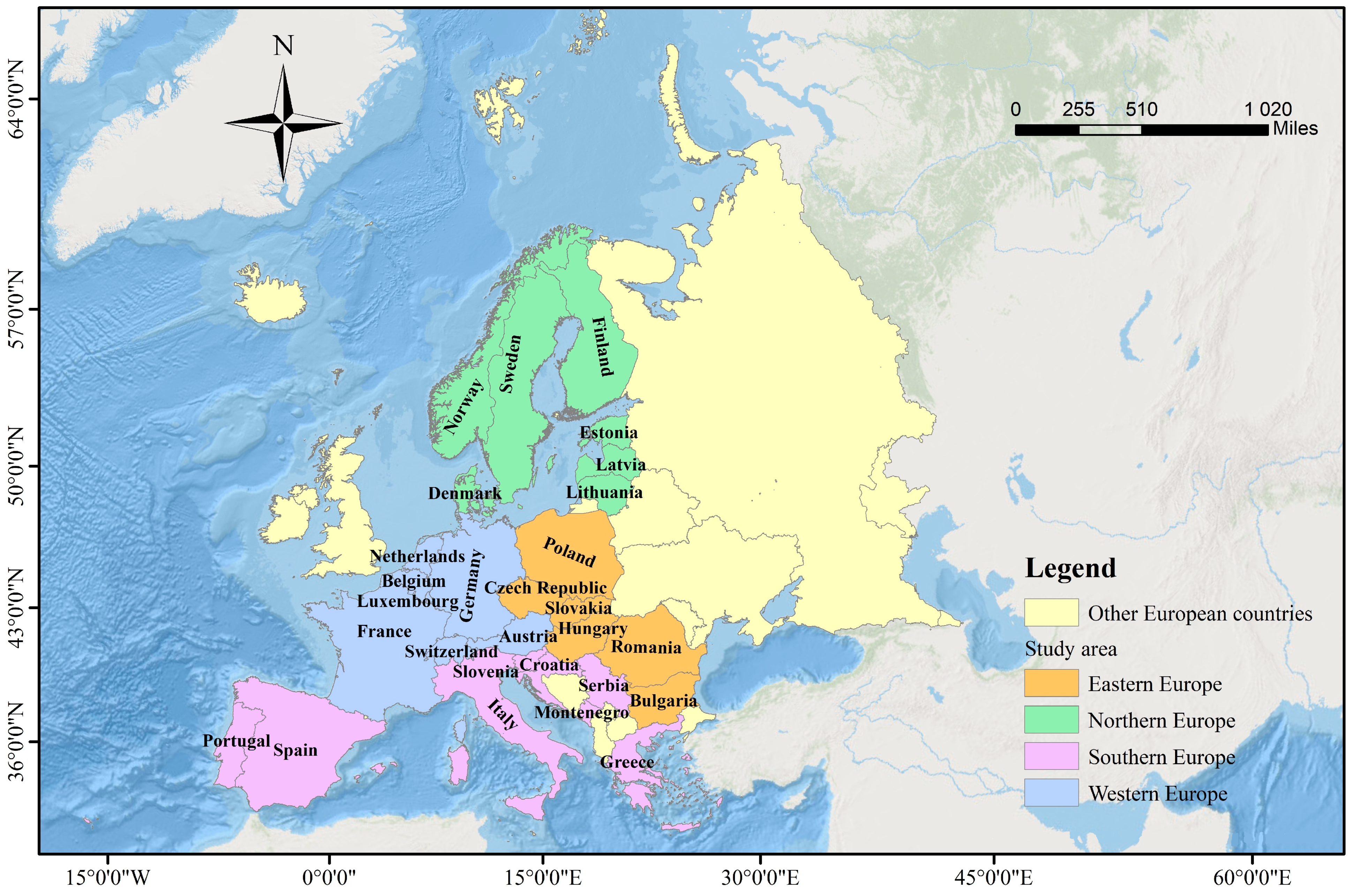
Figure 1. The geographical location of the study area.
Energies 17 00045 g001
Figure 2. Anomaly detection in electricity consumption for the Czech Republic.
Energies 17 00045 g002
Figure 3. Anomaly detection in electricity consumption for Spain.
Energies 17 00045 g003
Figure 4. Anomaly detection in electricity consumption for Poland.
Energies 17 00045 g004
Figure 5. Anomaly detection in the Netherlands for the year 2019 using the Isolation Forest (IF) method.
Energies 17 00045 g005
Figure 6. Anomaly detection in Germany for the year 2022 using the Isolation Forest (IF) method.
Energies 17 00045 g006
Figure 7. Temperature and precipitation distribution in the Netherlands for 2019 (Left) and Germany for 2022 (Right).
Energies 17 00045 g007
Figure 8. Anomaly detection in Italy for the year 2020 using the Isolation Forest (IF) method.
Energies 17 00045 g008
Figure 9. Spatial distribution map of maximum vulnerability. (a) The low temperature event in 2020; (b) The COVID-19 pandemic in 2020; (c) The high temperature event in 2022.
Energies 17 00045 g009
Figure 10. Spatial distribution map of duration. (a) The low temperature event in 2020; (b) The COVID-19 pandemic in 2020; (c) The high temperature event in 2022.
Energies 17 00045 g010
Table 1. Data sources and processing.
Data NameMeaningTime ScaleUnitData PreprocessingData Source
Temperature 1 day0.1 FUnit conversionhttps://www.ncei.noaa.gov/ (accessed on 14 April 2022)
Precipitation 1 day0.1 inch
Government stringency indexAn indicator of the strictness of the government’s epidemic prevention policy1 day https://ourworldindata.org/ (accessed on 3 March 2023)
Number of new COVID-19 casesNumber of newly reported cases1 day
The number of deaths due to COVID-19Number of newly reported deaths1 day
Epidemic prevention policyThe extent to which the government restricts internal movement/travel between regions and cities1 day
Geographical base map of European administrative divisions Projection transformationhttps://gadm.org/ (accessed on 30 September 2022)
Electricity consumption 15 min/1 hMWFill forward, statistical summaryhttps://transparency.entsoe.eu/ (accessed on 30 September 2022)
Disclaimer/Publisher’s Note: The statements, opinions and data contained in all publications are solely those of the individual author(s) and contributor(s) and not of MDPI and/or the editor(s). MDPI and/or the editor(s) disclaim responsibility for any injury to people or property resulting from any ideas, methods, instructions or products referred to in the content.