Abstract
With the objectives of achieving “peak carbon” and “carbon neutrality”, accurately quantifying the carbon emissions of road transportation becomes crucial. It is challenging to accurately describe the energy consumption of vehicles at both temporal and spatial scales from a macro perspective. Therefore, focusing on the quantitative model of vehicle micro energy consumption and road meso energy consumption, this paper reviewed and summarized the energy consumption model of road traffic in terms of data collection, quantification accuracy, and scope of application. Based on this analysis, this paper identifies the challenges of the current road traffic energy consumption model. Finally, we look forward to future research directions for studying quantitative models of energy consumption from road transportation.
1. Introduction
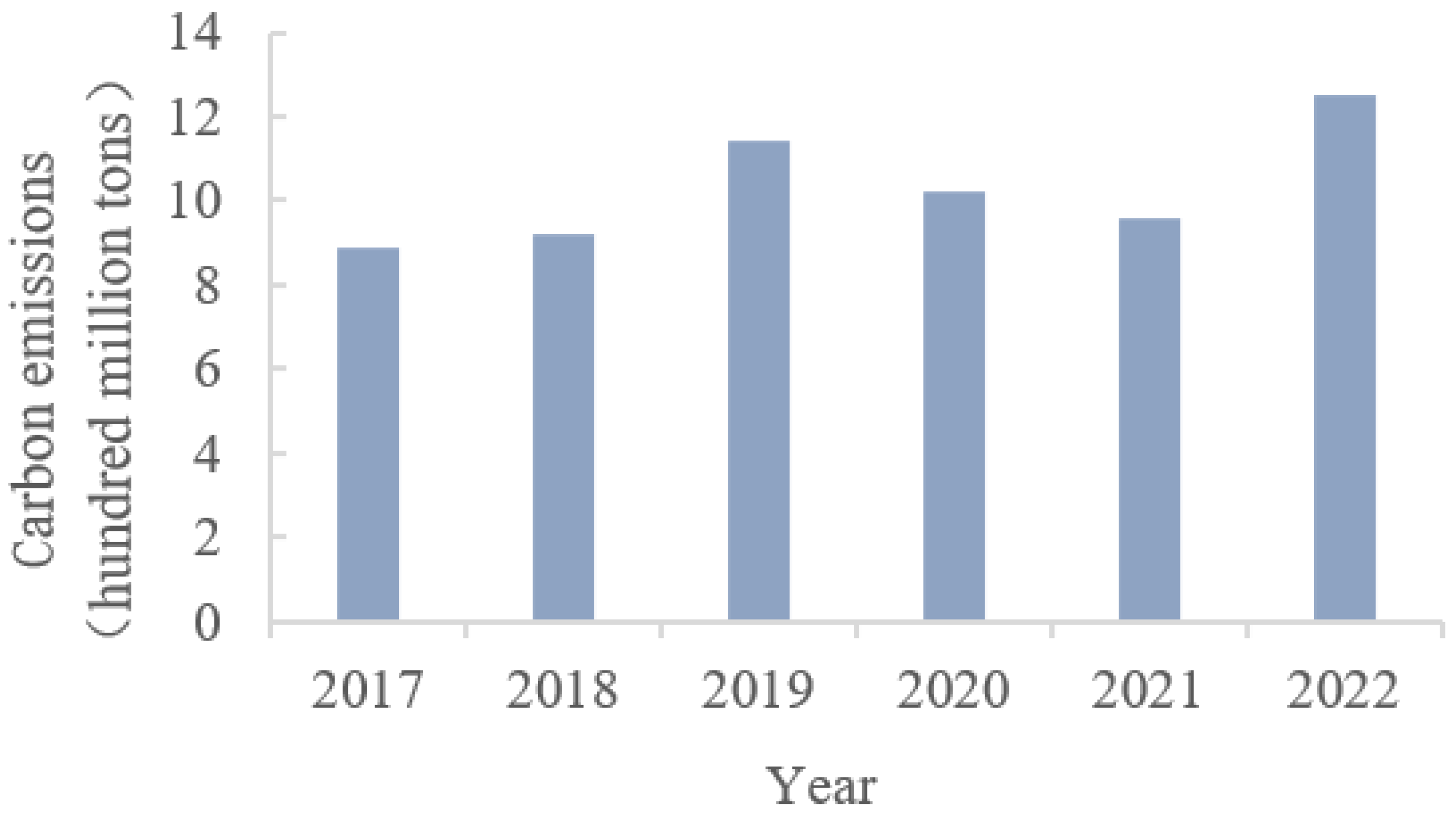
In September 2020, China proposed to “achieve peak carbon by 2030 and carbon neutrality by 2060” at the 75th United Nations Climate Conference. According to the International Energy Agency, carbon emissions from China’s transportation sector have grown rapidly in recent years. In 2021, China’s carbon emissions from the transportation sector dropped to 920 million tons due to COVID-19 but rapidly increased to 1.25 billion tons in 2022 [1]. Therefore, as one of the major contributors to China’s carbon emissions, road transportation is a key industry to achieving the “dual-carbon goal” (Figure 1).

Figure 1.
Carbon emissions of road transportation in China.
To achieve the “dual-carbon strategic goal”, obtaining comprehensive and accurate carbon emission data is essential. Accurately measuring the energy consumption of road transport serves as a fundamental prerequisite for mastering the trend of carbon emission, implementing emission reduction measures, and promoting sustainable development in road transport. China initiated the statistical accounting of carbon emissions in 2015, and has established an initial method for carbon emission accounting [2]. However, due to the complexity and dispersion of mobile emission sources in road transportation, selecting the appropriate quantitative model for road transportation energy consumption in different scenarios becomes crucial. Based on the extensive accumulation of energy consumption and driving data for light-duty vehicles, various models have been developed to quantify and predict energy consumption. Based on the developmental perspective and the level of practical application, these models can be categorized into microscopic, mesoscopic, and macroscopic models.
The study of energy consumption in the transportation sector is crucial for understanding and mitigating its environmental impact. In this context, the primary objective of this paper is to explore and provide a comprehensive overview of energy consumption models and shed light on the intricate dynamics of vehicle energy usage. This paper aims to consolidate and present research efforts conducted at the microscopic, mesoscopic, and macroscopic scales of road transportation energy consumption models. Existing reviews on quantifying fuel consumption have primarily focused on the micro level, but there is a noticeable absence of meso-level overviews concerning road networks. By studying the microscopic energy consumption model, we can simulate the energy consumption of individual motor vehicles within traffic flows on a second-by-second basis, and predict the instantaneous energy consumption of the vehicle. In addition, the mesoscopic energy consumption model primarily focuses on motor vehicles on urban road scales. Therefore, studying the mesoscopic energy consumption model can enhance our understanding of energy consumption models in road transportation. By doing so, we can contribute to the development of effective strategies and policies for optimizing energy efficiency in the transportation sector.
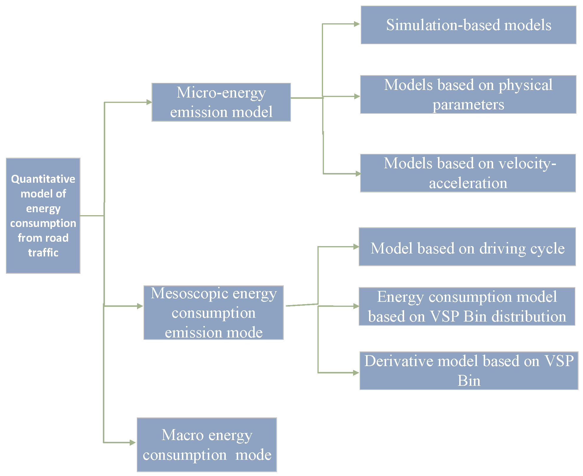
To achieve this goal, this paper will concentrate on synthesizing and analyzing research related to microscopic and mesoscopic energy consumption models. The microscopic and mesoscopic energy consumption models are shown in Figure 2. Through this approach, we hope to provide valuable insights into the underlying factors influencing energy consumption at these levels, facilitating more targeted interventions and improvements in energy efficiency within the road transportation sector.
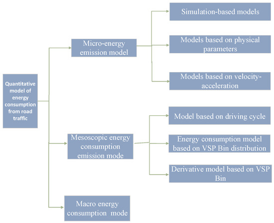
Figure 2.
Microscopic and mesoscopic modelling of energy consumption.
The subsequent sections of this paper will delve into the various microscopic and mesoscopic energy consumption models and provide a comprehensive analysis of their methodologies, research findings, and applications. By consolidating and summarizing existing research, we aim to extract meaningful conclusions and look forward to future research directions for studying quantitative models of energy consumption from road transportation.
2. Macroscopic Energy Consumption Model
The macroscopic energy consumption model takes the overall traffic flow on the road network within a certain geographical area as the statistical object, and the time is usually measured in days, months, or years. The calculation method for traffic energy consumption is generally based on data such as the total number of trips and vehicle types obtained from traffic surveys for statistical calculations [3]. For example, a typical urban energy consumption calculation formula is:
In the formula, is the energy consumption of the k-th type of vehicle driven by the i-th type of fuel. is the inventory of the k-th type of vehicle driven by the i-th type of fuel. is the average annual operating distance (km) of the k-th type of vehicle driven by the i-th type of fuel; is the energy intensity () of the k-th type of vehicle driven by the i-th type of fuel.
Due to the high degree of aggregation of time and space in macroscopic energy consumption models, it is difficult for these models to depict changes in traffic energy consumption based on road sections. Therefore, they are usually only used for macro trend analysis and cannot be applied to intelligent transportation systems that emphasize real-time and refined control.
3. Microscopic Energy Consumption Models
The research on microscopic energy consumption models started the earliest, and primarily focuses on individual vehicles. These models aim to simulate the energy consumption of individual motor vehicles within traffic flows on a second-by-second basis. To develop microscopic energy consumption models, researchers utilize daily driving data collected from motor vehicles, as well as various configuration parameters specific to vehicles. By examining the relationship between these parameters and the energy consumption of the vehicles, valuable insights can be gained. For instance, researchers analyze the collected instantaneous speed data with time granularity accurate to seconds. They use the data to calculate important metrics such as acceleration, deceleration, and average Vehicle Specific Power (VSP). They then combine this data with the vehicle’s inherent parameters, including weight and displacement, to predict the instantaneous energy consumption of the vehicle. Depending on the parameters chosen for the model, microscopic energy consumption models can be categorized into three types: models based on physical parameters, models based on speed–acceleration, and models based on motor vehicle power demand.
The research efforts of microscopic energy consumption models have laid a solid foundation for subsequent studies of mesoscopic and macroscopic energy consumption modeling. The representative models are shown in Table 1.

Table 1.
Representative microscopic energy consumption model parameters.
3.1. Models Based on Physical Parameters
The earliest development of power-based fuel consumption models was proposed by Post in 1984 [4], and improved by Akcelik and Biggs in 1989 [5]. An and Ross made further modifications in 1993 [6]. Wong’s [7] power-based fuel consumption model, based on previous work, is:
Among them, is the fuel consumption rate at time ; is the specific fuel consumption rate and varies with the engine status; is the engine friction pressure; is the engine speed; is the engine displacement; is the power of the transmission system; is the driving resistance of the vehicle; m is the vehicle mass; is the vehicle acceleration; and is the vehicle speed. is the gear ratio and is the efficiency of the transmission system. The friction pressure of the engine is generally proportional to the engine speed, but the mathematical relationship is difficult to obtain, so it is generally considered a constant.
On the basis of Wong, Hesham A. Rakha et al. from Virginia Tech established the Virginia Tech Comprehensive Power-Based Fuel Consumption Model (VT-CPFM), which can be calibrated by car manufacturers based on publicly available car parameters. This model solves the problem of previous fuel consumption models requiring real vehicle testing and calibration difficulty [8]. The model is shown in follow equations.
Among them, , , , and , , is the fuel consumption model constant, which can be calibrated using the vehicle’s public parameters, and is the engine idle speed.
3.2. Models Based on Physical Parameters
The Comprehensive Modal Emissions Model (CMEM) [9,10] is a typical application of physical parameter-based modeling, developed by the University of California, Riverside. Based on the power demand of a motor vehicle, the CMEM calculates the engine load using the vehicle’s parameters, instantaneous driving parameters, etc., then combines the air-fuel ratio and engine speed to calculate the vehicle’s energy consumption. Its calculation formula is shown below:
Ptrac denotes the traction power required to move the vehicle (kw); v is the instantaneous speed of the vehicle (m/s); a denotes the instantaneous acceleration of the vehicle (m/s2); and m is the vehicle gravity (kg). g denotes the gravitational acceleration, taken as 9.81 m/s2; grade is the road gradient, dimensionless; A, B and C are the rolling resistance coefficient, the velocity correction factor, and the wind resistance coefficient, dimensionless; ε denotes the vehicle driveline efficiency, dimensionless; and Pacc denotes the power (kw) of the vehicle’s ancillary equipment such as air conditioning. A conversion factor of 0.447/1000 is used to convert the emission factor to the correct units.
The CMEM (Comprehensive Modal Emission Model) has been widely applied in the research of energy consumption, leading to abundant findings both domestically and internationally. For instance, Zihan K [11], utilized the CMEM model to quantify and analyze the fuel consumption of individual vehicle trajectories and road networks. In addition, it was verified that the model achieved an accuracy rate exceeding 90%. Similarly, based on the CMEM, Zhao Xinran [12] constructed an emission model for motor vehicles and validated the model using driving patterns, theoretical parameter settings, and tailpipe emissions. Building upon the CMEM, Wang Xiaoning [13] modified the mass parameters, speed parameters, transmission efficiency parameters, and acceleration parameters to establish an exhaust emission model specifically applicable to diesel buses in China.
From these existing studies, it is evident that the energy consumption model based on physical parameters offers clear physical interpretations. When detailed and accurate parameters are available, the model can achieve relatively high accuracy. However, it also exhibits some notable drawbacks. The model relies on an extensive set of parameters, which are complex. In fact, its application necessitates a calibration of up to 46 parameters, requiring a substantial amount of data to support it. Consequently, the CMEM is typically deemed suitable for experimental environments.
3.3. Models Based on Velocity–Acceleration
The input parameters of the velocity–acceleration-based energy consumption model are relatively simple and are analyzed only on the basis of velocity and acceleration, which are mainly modeled using two-dimensional matrices of velocity and acceleration. The more typical energy consumption model based on velocity and acceleration is the VT-Micro model [14], and the calculation formula is:
where denotes the rate of instantaneous energy consumption in mg/s; is the model regression coefficient when accelerating or uniform speed; denotes the model regression coefficient when decelerating; denotes the instantaneous speed of the vehicle in m/s; and denotes the instantaneous acceleration of the vehicle in m/s2.
To address the problem of traffic emission quantification at roundabout intersections, Qingfang Yang [15] constructed a fuel consumption estimation model at roundabout intersections based on the VT-micro model combined with the traffic flow parameter model. A Elkafoury [16] investigated the distribution of time intervals of passenger cars and heavy-duty vehicles using the VT-micro model, and by calculating the individual vehicle CO emission coefficients to reveal the relationship between vehicle speed and CO emission coefficients. Based on the VT-micro model, Shaowei [17] numerically simulated the fuel economy and exhaust emission of traffic flow, and the results showed that the cooperative adaptive cruise control (CACC) strategy can improve the mobility, fuel economy, and exhaust emission performance of road traffic.
The advantage of the speed–acceleration-based energy consumption model is that it can be combined with computer simulation software or geo-location equipment to analyze historical data, but the model does not consider the road conditions as well as the vehicle’s own factors, it is completely detached from the motor vehicle’s engine power demand as well as the principle of fuel consumption, and the generalization ability is poor.
3.4. Simulation-Based Models
Microscopic traffic simulation models utilize individual vehicles as the primary unit for describing traffic behavior. A simulation-based model’s framework is built upon a vehicle-following model and a lane-changing model, which are further integrated into a vehicle path-selection model. Commonly used microscopic traffic simulation models include PTV-VISSIM (Germany), The Multi-Agent Transport Simulation (Germany), TransModeler (USA), AIMSUN (Spain), Simulation of Urban Mobility (Germany), and others.
The output of the micro-traffic simulation model, specifically the vehicle trajectory, can be directly fed into the micro-vehicle emission model. This allows for estimating the characteristics of vehicle operating conditions and refining the model structure and age distribution of vehicles.
4. Mesoscopic Energy Consumption Models
The energy consumption quantification model based on mesoscopic driving parameters utilizes instantaneous driving data series collected from motor vehicles on a specific road segment with a fixed length (1–10 km) or duration (1–30 min). Subsequently, it statistically calculates relevant mesoscopic model parameters such as average speed, average acceleration, deceleration, etc. and investigates their relationship with the average energy consumption value. Unlike microscopic energy consumption models, the mesoscopic energy consumption model primarily focuses on calculating energy consumption for motor vehicles on urban roads. Current research is mainly applied in the fields of “energy conservation and emission reduction” and “green navigation”. The prevailing research approach involves establishing an energy consumption calculation model that incorporates road traffic flow and physical structure. The inputs are parameters capable of accurately describing the mesoscopic driving state (e.g., average speed, acceleration, and deceleration speed). Studies on meso-level energy consumption models reveal that the energy consumption of motor vehicles is not solely influenced by instantaneous driving parameters. That is, a high speed at a specific moment does not necessarily correspond to an immediate increase in energy consumption. Rather, factors such as historical driving speed, acceleration and deceleration trends, and road structure all contribute to energy consumption. Therefore, it is crucial for current studies to identify an appropriate model that adequately describes the variation in vehicle driving states while also integrating roadway physical structure information.
Typical mesoscopic energy consumption models can be classified into three categories: models based on driving cycles, energy consumption models based on the Vehicle Specific Power bin distribution of motor vehicles, and models based on road characteristics and motor vehicle driving characteristic data. Table 2 illustrates the specific categories of well-established mesoscopic energy consumption models.
Table 2.
Typical mesoscopic energy consumption models.
Based on these typical mesoscopic energy consumption models, researchers have many applications. Table 3 illustrates some typical applications.
4.1. Models Based on Driving Cycles
A driving cycle represents the fluctuation of instantaneous speed in a specific vehicle, comprising a series of consecutive second-by-second speeds. Typically, a driving cycle lasts approximately 1500 s, which is relatively lengthy in time, and the driving cycle covers a larger number of vehicles [18,19]. The driving cycle-based model employs the FTP as the fundamental driving cycle, and utilizes a testing program to evaluate the exhaust emissions of motor vehicles. It then combines the collected road traffic data (e.g., road type, average traffic speed, etc.) and calculates the vehicle’s tailpipe emission factor. The tailpipe emission factor denotes the quantity of pollutants emitted per unit distance, commonly measured in grams per kilometer (g/km). Presently, the driving cycle-based energy consumption model is applied to the realm of tailpipe emission control.
The MOBILE model [20,21], developed by the United States in the 1960s, is the most prominent driving cycle-based energy consumption model. Its primary objective is to analyze the tailpipe emissions of vehicles in various operating conditions, thereby facilitating the control of tailpipe emissions and the enhancement of air quality. Over several decades of development, the structure and functionality of the MOBILE model have become highly refined, attracting extensive research by scholars both domestically and internationally. For instance, Gao Jun [22] used the MOBILE model 6.2 to investigate the pollutant emission characteristics of motor vehicles in Wuhan. This study calculated the emission factors of different vehicles, and assessed the pollutant emissions and distribution among various vehicle models in Wuhan. Hongjie Ma et al. (2014) [23] from Tianjin University focused on the impact of acceleration behavior on fuel consumption in response to the stop-and-go characteristics of urban buses.
The energy consumption model based on driving cycles has reached a relatively advanced stage in terms of theoretical maturity. Those models enable the characterization of both road characteristics and the energy consumption of motor vehicles under specific road conditions. Due to the extended duration of the driving cycle (approximately 1500 s) and the considerable distance covered by vehicles during the cycle, the coarse spatial resolution has minimal impact on analyzing energy consumption in normal straight-road configurations. However, the driving cycle-based model inadequately captures energy consumption and vehicle emissions under more intricate road structures, such as signalized road sections or areas near bus stops, due to the variability of driving conditions. Consequently, models based on driving cycles generally fail to accurately represent energy consumption and vehicle emissions under more detailed road structures, like signalized roads or roads in proximity to bus stops.
4.2. Models Based on the Vehicle Specific Power Bin Distribution
In order to further reduce the temporal and spatial granularity of energy consumption models and to improve the accuracy of the models, many researchers have turned their attention to methods based on the distribution of Vehicle Specific Power (VSP). The VSP (Vehicle Specific Power), which originated at the University of Massachusetts Institute of Technology (MIT) and was proposed by Jiménez Palacios, is defined as the value of the power output of the motor vehicle engine for moving an object with one ton of the value of the power output of a motor vehicle engine for moving an object of mass (including the engine itself) in kw/t [24]. Its calculation formula is shown below; since the calculation process of VSP takes into account factors such as the road gradient, speed, acceleration, etc., it can be a good reflection of the power demand of the vehicle in order to overcome the resistance to do work to meet the potential and kinetic energy of the vehicle, and the correlation with energy consumption is stronger than that of speed and acceleration.
denotes the power required to acquire the kinetic potential energy of the motor vehicle; denotes kinetic energy and denotes potential energy; denotes rolling resistance; denotes aerodynamic resistance; v denotes traveling speed; and m denotes the vehicle weight.
Expanded from the equations for kinetic energy, potential energy, and rolling resistance, as shown in Equation (5):
denotes the acceleration; denotes the rolling mass coefficient; denotes the road gradient; denotes the gravitational acceleration; denotes the coefficient of rotational resistance; denotes the air density; denotes the coefficient of wind resistance; denotes the cross-sectional area of the vehicle; and denotes the velocity of the headwind of the vehicle.
Peng Fei [25] proposed a model to measure energy consumption and carbon emissions factors in hybrid vehicles. This model utilized the VSP distribution as a parameter to characterize the coupled relationship between energy consumption, emissions, and driving conditions. The study found that the average relative errors between the model’s results and actual values were 3.7% and −1.7% for urban and high-speed driving conditions, respectively. Based on the VSP, Ye, Qianwen [26] estimated the potential energy savings of an optimization model called the Vehicle Queue Guiding Strategy (VPGS) at intersections. Chen, Qi [27] developed a fuel consumption prediction model for various speed intervals by incorporating traffic operation status and making corrections based on variables that have a significant impact on vehicle fuel consumption.
Related research has shown that the VSP interval distribution can effectively cover changes in the driving state of motor vehicles. Specifically, when a vehicle drives on a certain type of road at a given average speed, the pattern of changes in its driving state tends to resemble the distribution of VSP. Furthermore, when motor vehicles drive on the same type of road at the same speed, the distribution of VSP follows a normal distribution. Compared to the MOBILE model, the VSP-based model offers finer time granularity (20 s for non-expressways and 60 s for expressways) and higher accuracy in calculating energy consumption. However, the VSP-based energy consumption model only considers the road gradient as a factor for road conditions. It differentiates between straight and sloping roads, as well as roads of different grades. But it fails to capture the spatial granularity required and reflect changes in energy consumption values under more detailed road structures, such as signalized road sections or those near bus stops.
4.3. Derivative Models Based on VSP Bin
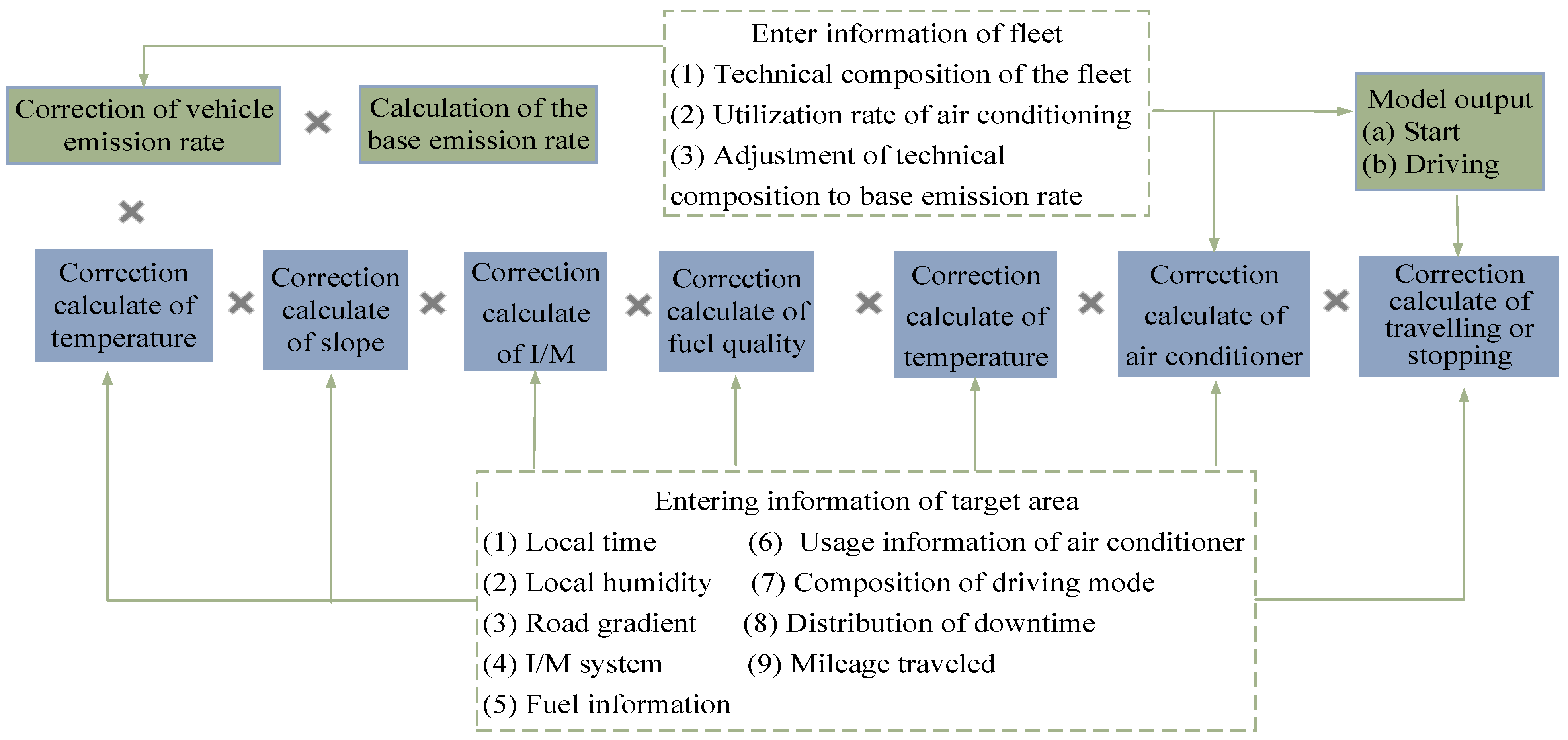
Derivative models based on VSP bin mainly include the MOVES model and the IVE model. The MOVES model is based on a large amount of local historical data in the U.S., which can not only be used to predict the energy consumption and emissions of each state except California, but can also be used to delineate the region or specify a period of time to calculate the energy consumption and emissions within the regional scope [28,29,30]. The main structure of the model is shown in Figure 3.
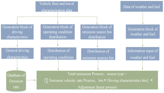
Figure 3.
The structure of the MOVES model.
The MOVES model calculates energy consumption and emission factors of motor vehicles based on their operating modes. These operating conditions are classified into acceleration, braking, uniform speed, and idling, which can be represented by the distribution of the Vehicle Specific Power (VSP) bin. By utilizing the VSP bin distribution, the MOVES model provides more accurate estimates of a motor vehicle’s energy consumption and emissions compared to methods solely based on speed, acceleration, and other traffic behavior parameters. In addition, the MOVES model also offers a more detailed description of changes in driving behavior resulting from traffic management strategies. However, it is important to note that the application of the MOVES model is currently limited to U.S. states and heavily relies on local data, making its localized adoption quite challenging.
The International Vehicle Emission Model was jointly developed by the Center for Environmental Research and Technology (CE-CERT) at the University of California, Riverside, the Global Sustainable Systems Research (GSSR), and the International Sustainability Research Center (ISSRC). The IVE model shares a similar computational approach with the MOVES model [31]. It primarily serves as a technical support tool for emission detection in developing countries, as depicted in Figure 4. However, due to the large number of input parameters required by the IVE model, its widespread application in regions with imperfect traffic data collection systems is difficult. Although the model comes preloaded with data from various countries and regions, including Beijing, Shanghai, and Pune, India, the data have not been updated in recent years (the latest data for Beijing is from 2007) [32]. Therefore, the accuracy of the model is difficult to guarantee.
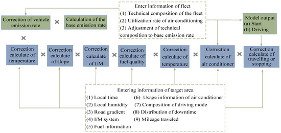
Figure 4.
The structure of the IVE model.
In recent years, there has been significant progress in the development of the MOVES model and the IVE model, leading to numerous research studies conducted by scholars. For instance, Shan Xiaonian [33] proposed a method to localize the correction of the MOVES model in China, considering the varying vehicle emission standards and testing conditions in the country. A case study was conducted using the corrected model. Feng Yusong [34] developed the Xi’an localization module of the MOVES model by analyzing vehicle driving cycles within different speed intervals. The localized model was then compared through the analysis of actual vehicle emission data. Xu Yaofang et al. [35] established a distribution model for the operating mode (i.e., driving mode) of motor vehicles, associating the two input parameters of average speed and road grade with the VSP distribution to determine the road driving mode and achieve the prediction of the emissions of vehicles passing through road sections. The time granularity of its calculation is 20 s (non-expressway) and 60 s (expressway), and the average speed range is refined to 2 km/h and 1 km/h. Compared to models based on driving cycles such as MOBIL/MOVES, models based on VSP distribution have finer calculation granularity and higher model accuracy, which can better adapt to the monitoring requirements of dynamically changing road networks. However, currently implemented models based on VSP distribution (including other similar models) can only calculate energy consumption and emissions based on road grade, and still do not achieve the fine-grained monitoring of road microstructure. We know that under the same level of road, there are significant differences in energy consumption between different structural sections. For example, on urban expressways, when passing through closed sections and sections with entrances and exits at the same average speed, the average energy consumption can differ by more than 1 L/100 km. However, existing mesoscopic energy consumption models cannot identify the fuel consumption differences caused by this structural difference.
Table 3.
Typical applications.
Table 3.
Typical applications.
| Typical Models | Typical Applications | |
|---|---|---|
| Models based on driving cycles | MOBILE Model | Gao Jun [22] used the MOBILE model 6.2 to investigate the pollutant emission characteristics of motor vehicles in Wuhan. Hongjie Ma et al. (2014) [23] from Tianjin University focused on the impact of acceleration behavior on fuel consumption in response to the stop-and-go characteristics of urban buses. |
| Models based on Vehicle Specific Power bin distribution | Vehicle Specific Power Model | Peng Fei [25] proposed a model to measure energy consumption and carbon emissions factors in hybrid vehicles. Based on the VSP, Ye, Qianwen [26] estimated the potential energy savings of an optimization model called the Vehicle Queue Guiding Strategy (VPGS) at intersections. Chen, Qi [27] developed a fuel consumption prediction model for various speed intervals by incorporating traffic operation status and making corrections based on variables that have a significant impact on vehicle fuel consumption. |
| Derivative model based on VSP bin | MOVES Model | Han Xiaonian [33] proposed a method to localize the correction of the MOVES model in China. Feng Yusong [34] developed the Xi’an localization module of the MOVES model by analyzing vehicle driving cycles within different speed intervals. |
| IVE Model | Xu Yaofang et al. [35] established a distribution model for the operating mode (i.e., driving mode) of motor vehicles, associating the two input parameters of average speed and road grade with the VSP distribution to determine the road driving mode and achieve the prediction of the emissions of vehicles passing through road sections. |
5. Conclusions
The selection of methods to quantify energy consumption and carbon emissions in road transportation plays a crucial role in promoting energy conservation and emission reduction. However, the complexity of the road transportation system and the dynamic nature of transportation carbon emissions as a mobile carbon source make carbon emission measurement more challenging. Nevertheless, accurate quantification of road traffic energy consumption and carbon emissions is essential for setting emission reduction targets and implementing effective measures. As a result, researchers worldwide have conducted extensive studies on micro-level vehicle energy consumption (focusing on individual vehicles and exploring the relationship between driving data and energy consumption) and meso-level road energy consumption quantification (analyzing energy consumption patterns for specific road sections or time periods). This paper provides a comprehensive review and summary of these two types of models in terms of examining data collection methods, quantification accuracy, and the scope of application.
Firstly, the models based on microscopic energy consumption, which emerged earlier, have reached a relatively advanced stage of research. Typical research methods include the statistical analysis of historical data and power demand modeling. The findings and methods of the microscopic energy consumption model can offer theoretical support and methodological guidance for research at both the meso and macro levels. However, the micro-level model requires more input parameters and provides a more detailed analysis, making it suitable for calculating energy consumption under specific traffic conditions. Due to limitations in current traffic information collection, the application of the micro-level model in road energy consumption monitoring is challenging.
The mesoscopic energy consumption model primarily focuses on calculating energy consumption in urban road scenarios, which holds significant application value in the domains of environmental protection, navigation, energy saving, and emission reduction. Currently, the prevalent research approach involves establishing an energy consumption model with inputs related to road conditions and the road environment, utilizing parameters that accurately describe the mesoscopic driving state such as stopping, accelerating, decelerating, etc. While factors like weather and vehicle age also impact motor vehicle energy consumption at the mesoscopic level, it is crucial to consider the driving state of the vehicles. Statistical analysis reveals that higher vehicle speeds lead to increased fuel consumption, while frequent acceleration and deceleration at lower speeds also contribute to higher fuel consumption. This shows that relying solely on speed or acceleration and deceleration parameters for modeling purposes is inaccurate. Unfortunately, the commonly used models still suffer from low accuracy, limited generalization ability, and difficulties in localization. Thus, the challenge lies in finding a parameter that accurately captures the driving state of a motor vehicle and predicts energy consumption by combining it with road conditions and types of roads.
Considering the aforementioned issues in the meso-micro quantitative energy consumption model, coupled with the recent advancements in smart cities and emerging technologies like networking, the development and application of large-scale driving data collection has become feasible. To achieve more refined carbon emission quantification, future research in this field may focus on the following directions:
- For the microscopic energy consumption model, leveraging massive driving data and analyzing the impact of different driving parameters on energy consumption. This involves identifying various typical driving patterns and incorporating the physical attributes of the vehicle (weight, age, displacement, etc.). The goal is to establish a more widely applicable and universally quantifiable energy consumption model based on easily collectible data parameters.
- For the mesoscopic energy consumption model, considering a substantial amount of actual vehicle driving data and investigating different driving modes based on the historical driving data of vehicles. An in-depth analysis of how different physical road structures affect vehicle energy consumption will be conducted. This allows for the further exploration of energy consumption patterns for light vehicles under various road structure conditions. Ultimately, an energy consumption quantification model will be established, incorporating inputs related to the driving parameters of vehicles as well as the physical structure of the roads.
Author Contributions
Conceptualization, S.L. and Y.L.; methodology, Y.C., S.L. and Y.L.; writing—original draft preparation, S.L. and Y.L.; visualization, S.L. and Y.L.; writing—review and editing, Y.C., S.L. and Y.L.; supervision, Y.C., S.L. and Y.L. All authors have read and agreed to the published version of the manuscript.
Funding
This research received no external funding.
Data Availability Statement
All data included in this study are available upon request by contact with the corresponding author.
Conflicts of Interest
The authors declare that they have no conflict of interest with respect to the research, authorship and/or publication of this article.
References
- Feng, J.; Shidong, Y.; Hongying, Z. Digital electric travel mode facilitate the realization of “carbon neutrality”—Analysis on carbon reduction data of 2018–2021 based on Didi ChuXing. World Environ. 2021, 5, 52–55. [Google Scholar]
- Ma, J.; Chai, Y.W.; Liu, Z. The Mechanism of CO2 Emissions from Urban Transport Based on Individuals’ Travel Behavior in Beijing. Acta Geogr. Sin. 2011, 66, 1023–1032. [Google Scholar]
- Zhu, S. Comparison of urban transport energy consumption and greenhouse gas emissions between Beijing and Shanghai. Urban Transp. 2010, 3, 58–63. [Google Scholar]
- Post, K.; Kent, J.H.; Tomlin, J.; Carruthers, N. Fuel consumption and emission modelling by power demand and a comparison with other models. Transp. Res. Part A Gen. 1984, 18, 191–213. [Google Scholar] [CrossRef]
- Akcelik, R. Efficiency and drag in the power-based model of fuel consumption. Transp. Res. Part B Methodol. 1989, 23, 376–385. [Google Scholar] [CrossRef]
- Feng, A.; Ross, M. A Model of Fuel Economy and Driving Patterns; SAE Technical Paper; SAE International: Warrendale, PA, USA, 1993. [Google Scholar]
- Wong, J.Y. Theory of Ground Vehicles; John Wiley & Sons: Hoboken, NJ, USA, 2001. [Google Scholar]
- Park, S.; Rakha, H.; Ahn, K.; Moran, K. Virginia tech comprehensive power-based fuel consumption model: Model development and testing. Transp. Res. Part D Transp. Environ. 2011, 16, 492–503. [Google Scholar]
- Scora, G.; Barth, M.; An, F.; Younglove, T.; Levine, C. Comprehensive Modal Emissions Model (CMEM); Version 2.0; User’sGuide; University of California, Riverside: Riverside, CA, USA, 2000. [Google Scholar]
- Lima, E.P.; Demarchi, S.H.; Gimenes, M.L. Adaptation of CMEM modal emission model to the fleet of the city of Maringii, Parana State, Brazil. Acta Sci. -Technol. 2011, 33, 17–25. [Google Scholar]
- Kan, Z.; Tang, L.; Kwan, M.P.; Ren, C.; Liu, D.; Pei, T.; Liu, Y.; Deng, M.; Li, Q. Fine-grained analysis on fuel-consumption and emission from vehicles trace. J. Clean. Prod. 2018, 203, 340–352. [Google Scholar] [CrossRef]
- Zhao, X. Emission Model Research on Eco-routing Algorithm Based on Vehicle Exhaust. Ph.D. Thesis, Beijing Jiaotong University, Beijing, China, 2020. [Google Scholar]
- Wang, X.N.; Liu, H.Y.; Li, T.H.; Deng, K. The emission model of diesel bus based on CMEM in China. J. Harbin Inst. Technol. 2012, 44, 78–81. [Google Scholar]
- Rakha, H.; Ahn, K.; Trani, A. Development of VT-Micromodel for estimating hot stabilized light duty vehicle and truck emissions. Transp. Res. Part D Transp. Environ. 2004, 9, 49–74. [Google Scholar] [CrossRef]
- Yang, Q.; Wang, L.; Zheng, L.; Meng, F. Traffic Emission and Fuel Consumption Model of Roundabout. J. Chongqing Jiaotong Univ. (Nat. Sci.) 2021, 40, 67–73. [Google Scholar]
- Elkafoury, A.; Negm, A.M.; Bady, M.F.; Aly, M.H. Modeling vehicular CO emissions for time headway-based environmental traffic management system. Procedia Technol. 2015, 19, 341–348. [Google Scholar] [CrossRef]
- Guo, L.; Zhao, X.; Yu, S.; Li, X.; Shi, Z. An improved car-following model with multiple preceding cars’ velocity fluctuation feedback. Phys. A Stat. Mech. Appl. 2017, 471, 436–444. [Google Scholar] [CrossRef]
- Fei, M. Vehicle Emission Characteristic Parameters-based Approach to the Development and Evaluation of Driving Cycles. Ph.D. Thesis, Beijing Jiaotong University, Beijing, China, 2007. [Google Scholar]
- Liu, J. Speed Correction Model for Vehicle Emissions and Fuel Consumption Based on VSP Distributions. Ph.D. Thesis, Beijing Jiaotong University, Beijing, China, 2010. [Google Scholar]
- EPA420-R-03-010; User’s Guide to MOBILE6.1 and MOBILE6.2: Mobile Source Emission Factor Model. U.S. Environmental Protection Agency: Washington, DC, USA, 2003.
- Gao, T. Sensitivity Analysis and Comparison of the Factors Affecting Vehicle Emission based on MOBILE. Ph.D. Thesis, Beijing Jiaotong University, Beijing, China, 2011. [Google Scholar]
- Gao, J.; Hu, H.; Xing, P.; Gang, L. Emission Characteristics of Pollutants from MotorVehicles in Wuhan Based on MOBILE 6.2. J. Taiyuan Univ. Technol. 2018, 49, 73–78. [Google Scholar]
- Ma, H.; Xie, H.; Chen, S.; Yan, Y.; Huang, D. Effects of Driver Acceleration Behavior on Fuel Consumption of City Buses; SAE Technical Paper; SAE International: Warrendale, PA, USA, 2014. [Google Scholar]
- Jimenez-Palacios, J.L. Understanding and Quantifying Motor Vehicle Emissions with Vehicle Specific Power and TILDAS Remote Sensing. Ph.D. Thesis, Massachusetts Institute Technology, Cambridge, MA, USA, 1999. [Google Scholar]
- Peng, F.; Song, G.; Yin, H.; Yu, L. Energy Consumption and CO2Emission Model for Hybrid Vehicles in Real Traffic Conditions. J. Transp. Syst. Eng. Inf. Technol. 2022, 22, 316–326. [Google Scholar]
- Ye, Q.; Chen, X.; Liao, R.; Yu, L. Development and evaluation of a vehicle platoon guidance strategy at signalized intersections considering fuel savings—ScienceDirect. Transp. Res. Part D Transp. Environ. 2019, 77, 120–131. [Google Scholar] [CrossRef]
- Chen, Q. The Study on Urban Road Fuel ConsumptionModel Based on Vehicle Specific Power. Ph.D. Thesis, North China University of Technology, Beijing, China, 2019. [Google Scholar]
- EPA-420-B-09-041; Motor Vehicle Emission Simulator (MOVES) 2010. U.S. Environmental Protection Agency: Washington, DC, USA, 2009.
- Chamberlin, R.; Swanson, B.; Talbot, E.; Dumont, J.; Pesci, S. Analysis of MOVES and CMEM for evaluating the emissions impact of an intersection control change. In Proceedings of the Transportation Research Board 90th Annual Meeting, Washington, DC, USA, 23–27 January 2011. [Google Scholar]
- Huang, G. Evaluation of Traffic Emissions at Microscopic Level Based on MOVES. Ph.D. Thesis, Beijing Jiaotong University, Beijing, China, 2011. [Google Scholar]
- Davis, N.; Lents, J.; Osses, M.; Nikkila, N.; Barth, M.J. IVE Model User’s Manual; Version 2.0; International Sustainable Systems Research Center—ISSRC: La Habra, CA, USA, 2008. [Google Scholar]
- Huo, H.; Yao, Z.; He, K.; Yu, X. Fuel consumption rates of passenger cars in China: Labels versus real-world. Energy Policy 2011, 39, 7130–7135. [Google Scholar] [CrossRef]
- Shan, X.; Liu, H.; Zhang, X.; Chen, X. Localization of Light-Duty Vehicle Emission Factor Estimation Based on MOVES. J. Tongji Univ. (Nat. Sci.) 2021, 49, 1135–1143+1201. [Google Scholar]
- Feng, Y. Establishment of MOVES—Xi’an Emission Model and Its Application of Pollution Evaluation. Ph.D. Thesis, Chang’an University, Xi’an, China, 2020. [Google Scholar]
- Xu, Y. Motor Vehicle Operation Mode Distribution Model for Traffic Network Emission Measurement. Ph.D. Thesis, Beijing Jiaotong University, Beijing, China, 2012. [Google Scholar]

Disclaimer/Publisher’s Note: The statements, opinions and data contained in all publications are solely those of the individual author(s) and contributor(s) and not of MDPI and/or the editor(s). MDPI and/or the editor(s) disclaim responsibility for any injury to people or property resulting from any ideas, methods, instructions or products referred to in the content. |
© 2023 by the authors. Licensee MDPI, Basel, Switzerland. This article is an open access article distributed under the terms and conditions of the Creative Commons Attribution (CC BY) license (https://creativecommons.org/licenses/by/4.0/).