Abstract
The intermittent and random nature of wind brings great challenges to the accurate prediction of wind power; a single model is insufficient to meet the requirements of ultra-short-term wind power prediction. Although ensemble empirical mode decomposition (EEMD) can be used to extract the time series features of the original wind power data, the number of its modes will increase with the complexity of the original data. Too many modes are unnecessary, making the prediction model constructed based on the sub-models too complex. An entropy ensemble empirical mode decomposition (eEEMD) method based on information entropy is proposed in this work. Fewer components with significant feature differences are obtained using information entropy to reconstruct sub-sequences. The long short-term memory (LSTM) model is suitable for prediction after the decomposition of time series. All the modes are trained with the same deep learning framework LSTM. In view of the different features of each mode, models should be trained differentially for each mode; a rule is designed to determine the training error of each mode according to its average value. In this way, the model prediction accuracy and efficiency can make better tradeoffs. The predictions of different modes are reconstructed to obtain the final prediction results. The test results from a wind power unit show that the proposed eEEMD-LSTM has higher prediction accuracy compared with single LSTM and EEMD-LSTM, and the results based on Bayesian ridge regression (BR) and support vector regression (SVR) are the same; eEEMD-LSTM exhibits better performance.
1. Introduction
With the increase in fossil fuel consumption and the impact of global climate change, renewable energy has become a focus topic worldwide [1,2]. Over the past decades, wind power has rapidly and drastically developed as a clean, sustainable alternative energy source. The more complex the time series, the greater the difficulty of model prediction, and wind power generation is highly uncertain due to its randomness, fluctuation, and intermittence, which brings great challenges to the accurate prediction of wind power and poses potential dangers to the safe and stable operation of the power system when integrated on a large scale [3,4]. Therefore, accurate wind power prediction is critical to ensuring the safe operation of the power system.
Research has shown that shallow machine learning wind power forecasting methods, such as the support vector machine (SVM) [5] and logistic regression (LR) [6] methods, are more accurate than traditional methods. Nevertheless, these models can only evaluate the fundamental characteristics of wind power time series. With time series data becoming more complex, traditional statistical models encounter difficulties in extracting pertinent data features and may not meet the accuracy standards required for prediction.
Advanced deep learning techniques can extract complex and hidden features from data, thereby achieving more accurate ultra-short-term wind power forecasting. The precision and efficacy of prediction models employing deep learning, particularly the recurrent neural network type known as LSTM, have been widely recognized [7,8]. Scholars [9,10,11] have compared and analyzed various wind power prediction methods based on LSTM, concluding that LSTM can improve prediction performance more than other techniques. However, a single LSTM prediction model has limitations, and its prediction performance makes it difficult to meet the prediction demand when predicting wind power with complex time series characteristics. Therefore, a combined model that utilizes LSTM to extract hidden time series information from different perspectives could improve wind power prediction accuracy. Combination models based on LSTM have proven effective in recent years [12].
To improve the accuracy of wind power prediction, researchers use empirical mode decomposition (EMD) to decompose time series into modal functions and residuals [13,14,15]. However, EMD may lead to modal confusion [16,17]. The EEMD approach is introduced to solve the problem, which decomposes the local characteristics of complex time series into multiple more stable and regular sub-sequences, thereby improving the prediction accuracy of the model [18,19,20]. However, generating more intrinsic mode function (IMF) components in highly complex data can significantly affect the prediction efficiency of the model.
To solve the problem of excessive prediction components in highly complex data situations, we propose an eEEMD method to reconstruct EEMD components by using information entropy. We use information entropy to determine the complexity of the time series, then reconstruct time series with similar complexity based on the difference coefficient. However, using the same model for different complexity components may not be the most effective way to optimize prediction performance. Therefore, we propose setting distinct training error targets based on the average values of the reconstructed components. This method can help minimize the possibility of over-learning or under-learning and ultimately improve wind power performance. The eEEMD-LSTM model combines the strengths of eEEMD and LSTM. The final experimental results demonstrate that the eEEMD-LSTM method outperforms other methods in terms of predicted results.
The contributions lie in two aspects: 1. An eEEMD method for time series decomposition is proposed, which can improve the prediction efficiency of the model. 2. Based on sub-sequences, an adaptive differential training method is proposed, ultimately effectively improving the prediction accuracy of the model. The rest of this article is organized as follows. In Section 2, the potential of the eEEMD method for time series decomposition is theoretically analyzed in detail. Section 3 elaborates on differential training based on the LSTM network. Section 4 provides the experiments and results analysis. Finally, Section 5 provides a summary of this article.
2. Wind Power Time Series Decomposition Method Based on eEEMD
Figure 1 shows wind power data collected from a wind farm in 2017, with a sampling interval of 15 min. These data exhibit intermittent and volatile behavior, posing challenges for accurate wind power prediction. However, the time series decomposition method provides a solution by extracting local features and decomposing complex time series features into simpler ones. This method can significantly enhance the accuracy of wind power prediction.
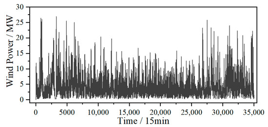
Figure 1.
Original wind power data.
2.1. EMD Method and EEMD Method
EMD is an effective technique for decomposing time series data into a set of IMF and residual waves. It is highly effective at extracting valuable information from complex time series and has been proven to enhance the accuracy and efficiency of time series-based prediction methods.
However, the EMD method may be prone to mode mixing, which can lead to unclear features in the IMFs or the decomposition of the same feature into multiple sub-time series. To address this limitation, EEMD was developed. EEMD decomposes the original time series into several sub-time series components, and the original sequence is the sum of all sub-sequences. Based on EMD decomposition, EEMD adds Gaussian noise in the decomposition process, which can effectively reduce the local feature aliasing phenomenon in the decomposition process, and is more empirical, adaptive, and intuitive. It has been successfully used to decompose time-frequency data from non-stationary and nonlinear time series across various fields. The EEMD algorithm is presented in Algorithm 1.
| Algorithm 1 EEMD algorithm |
| Initialization: , , |
| while to do |
| Add Gaussian noise to the original . |
| while to do |
| Find the local maximum and minimum values of the input. |
| Calculate the average of the two envelopes. |
| Calculate the difference according to and . |
| if the stop condition is met then |
| end while |
| Calculate the average of . |
| end while |
| return |
Where indicates that the value range of Gaussian noise of EEMD is 0.05; represents the range of the decomposition cycle’s numbers; represents the range of the number of sub-components. represent EEMD results; i = 1, 2, …, N; j = 1, 2, …, R.
It is important to consider that the EEMD decomposition method may not be the optimal selection for datasets containing substantial amounts of wind power data. This method tends to produce numerous IMFs, potentially decreasing the efficacy of wind power prediction.
2.2. Wind Power Decomposition with eEEMD
EEMD can reduce the modal confusion in EMD, but it will produce large quantum components when decomposing complex time series data, which will seriously affect the performance of wind power prediction.
To minimize the number of IMFs, it is crucial to understand the characteristics of each component group. The information entropy method comprehensively presents data information. The entropy weight method allocates weights based on information entropy, and even if negative values exist in the matrix, this method is still effective. However, this article aims to extract data information without weight assignments, using the entropy method’s information entropy and difference coefficient calculation method instead.
The entropy weight method objectively evaluates the amount of data information based on the entropy value. When the time series features are fully extracted, the entropy value is low, while when the sequence features in the component are unclear, the entropy value is high. The difference coefficient and entropy value reflect opposite characteristics, allowing for the reconstruction of information characteristics in the sub-sequence to control the number of sub-sequences. The sequence is reconstructed using the entropy and difference coefficient calculation formulas.
After calculating the information characteristics of each IMF group separately, redundant IMFs are reconstructed based on relevant characteristics. The reconstruction rules are combined with the decomposition method to produce the new eEEMD-reconstructed decomposition method, as shown in Algorithm 2.
| Algorithm 2 eEEMD algorithm |
| Initialization: , |
| while to do |
| if then |
| Re-standardize to a non-negative interval. |
| else |
| Calculate the proportion of the sample of . |
| if then |
| else |
| Calculate difference coefficient . |
| end while |
| Reconstruct to according to specific merger rules. |
| return , , |
Where is the result of EEMD; is the decomposition result of eEEMD; i = 1, 2, …, N; j = 1, 2, …, R.
This article introduces a new method called the eEEMD decomposition and reconstruction method to solve the problem of generating an excessive number of IMFs when EEMD decomposes large amounts of wind power data. This method combines information entropy and EEMD, and according to the characteristics of information entropy, determines the similarity of difference coefficients between subassemblies. To ensure best wind power prediction efficiency, a certain degree of reconstruction can be carried out.
However, it is important to note the limitations of the eEEMD reconstruction method. If the number of decomposed sub-sequences is less than R, a zero sequence is added to ensure that the number of sub-sequences remains R. If the number of decomposed sub-sequences exceeds R, the decomposition process is stopped. If R is too small, incomplete decomposition may occur, which will affect the subsequent component feature analysis. Conversely, if R is too large, the number of reconstructed sub-sequences may still be too high, making it difficult to limit the number of IMFs. Therefore, R should be adjusted according to the complexity of the data. We suggest that the interval size of M should be kept below 20 units for the same order of data.
It is important to remember that the difference coefficient in the same range may change from time to time during the reconstruction process. This means that if two or more sequence components exist in different intervals between two sequences and the difference coefficient values fall within the same interval, the two sequence components should be reconstructed into different new sequence components.
Based on the entropy calculation results, it is obvious that the characteristics of the components can be significantly different. Attempting to use a unified model to predict the IMFs may result in under-learning or over-learning. To alleviate this problem, the eEEMD decomposition method decomposes the original wind power data gradually, from high to low frequency. It is worth noting that the high-frequency sub-component exhibits a substantially lower average value, while the low-frequency sub-component has a significantly higher average value. Consequently, the average value characteristics of the sub-components can be leveraged to distinguish between the prediction models of distinct components.
3. eEEMD-LSTM Method Based on Sub-Model Differential Training
After decomposing the complex wind power data through eEEMD, wind power prediction can meet the basic requirements for wind power prediction using LSTM. However, due to the obvious differences in sub-model features, it is difficult to obtain the optimal prediction results using the same model, so a sub-model differentiation training rule for different sub-models is proposed.
3.1. LSTM Network
Recurrent neural networks (RNNs) have been exploited by researchers in various applications to extract hidden nonlinear and non-static features. A simple RNN consists of three layers: an input layer, a hidden layer, and an output layer. Compared with the RNN, the basic LSTM also consists of three layers, but the hidden layer of the LSTM adds some threshold units for controlling information transmission, which gives the neural network a unique memory mode.
The LSTM can overcome the RNN disadvantage of the vanishing gradient. It consists of recurrent network units that maintain the short-term and long-term duration values, which use memory cells to store information and are better at discovering and eliminating long-term context. The memory cell helps to train and store the previously predicted time information and propagate it to the network when necessary. These units are the input unit, forget unit, and output unit. The information that resides in memory depends on the high activation results; if the input unit has high activation, the information is stored in the memory cell. Similarly, if the output unit has high activation, it will transmit the information to the next neuron. Forget unit has high activation and it will erase the memory cell.
The specific workflow of the LSTM network is in Figure 2.
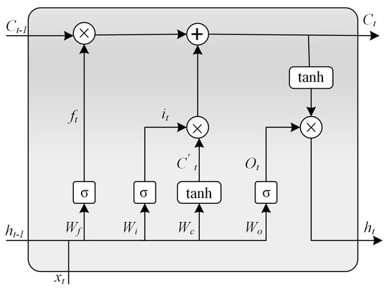
Figure 2.
Structure of LSTM.
In the lth layer, the input of each hidden layer includes the present input , the state of the hidden layer and the output . During calculation, the output is derived and the current state is updated to . , , respectively represent the values of the input gate, forget gate, and output gate. , , , indicate the weights matrix in different gates, and , , , are their corresponding bias terms. and denote the sigmoid function and hyperbolic tangent function, respectively.
The input gate of the cell uses the Logistic sigmoid function to decide whether to store the current input and the new cell state in the memory. Similarly, the forget gate of the cell uses the Logistic sigmoid function to decide whether to remove the previous cell state from the memory. The new cell state is determined by the number of old cell states to be forgotten and the number of new information to be included. The output gate uses the Logistic sigmoid function to filter information from the current input, previous cell state, and previous hidden state. The new hidden state is calculated as the Hadamard product between the output gate value and the function value of the current state. Finally, the output of the memory cell is calculated from the hidden state cell state. The pseudo-code of the classic LSTM is shown in Algorithm 3 [21].
| Algorithm 3 LSTM algorithm |
| Initialization: Initialize the hyper parameters, including Uf, Ui, Uc, bf, bi, bo, and bc, set ho = 0, Co = 0. |
| For to do |
| Calculate forget gate ft, decide how much information to forget. |
| Calculate input gate it, determine the information to be stored. |
| Calculate output gate Ot, filter information. |
| Calculate temporary state C′t. |
| Calculate current state Ct, update cell state. |
| Calculate output ht. |
| return |
3.2. Differential Training Based on Sequence Mean
Using the difference coefficient to reconstruct the component can reduce the calculation of the model to some extent. During the same data training process, the network error target setting can affect the prediction performance of the model. To minimize the prediction error, it is necessary to adjust the network error target. However, please note that there are significant differences in signal sizes between the different sub-components, so it is unreasonable to use a uniform error target for all sub-components.
To prevent over-learning or under-learning when training different sub-component signals under the same error metric, it is equally important to rely on the feature relationships between sequences. Differentiated training of the model can make the same model have different training performances and meet the prediction requirements of different sub-sequences. According to the principle of EEMD decomposition, it can be concluded that the decomposition components change regularly from high frequency to low frequency, with the mean of high-frequency components being significantly smaller and the mean of low-frequency components being significantly larger. The mean can be used to distinguish different components. Therefore, the average value of each component can be used to adaptively adjust the erroneous target of each network.
Based on the reference error target, adjust the training error of the model according to the difference in the average value of each component signal. Due to the possibility of small differences in average amplitudes of different component signals, an exponential function is utilized to set the strategy. It is important to establish an upper limit for the adjustment coefficient of the error target to prevent the error target adjustment magnitude from becoming too large or unreasonable due to the differences in average values and set the Kmax limit. Following this, the training error target of each component is adjusted differentially, and then the component model network is trained and tested. As shown in Equation (1).
where errorj is the training error of IMFj; errorq is the training error of IMFq, and Avgq is the mean of IMFq; Avgj is the mean of IMFj; xi,j is the decomposition data of sub-components; Kmax is the maximum adaptive adjustment coefficient.
Because it takes a lot of time to input wind power data into the network for forecasting after decomposition and reconstruction, online training is insufficient to ensure the efficiency of wind power prediction. Therefore, an offline training model is used for training and learning.
3.3. Wind Power Prediction Based on eEEMD-LSTM
With the annual expansion of wind power generation scale, higher requirements have been put forward for the accuracy and efficiency of wind power prediction. The traditional simple wind power prediction method can no longer meet the requirements of prediction performance. Therefore, the combination prediction method of the EEMD decomposition algorithm and LSTM has been widely considered.
In highly complex data scenarios, the LSTM prediction method is superior to other deep learning methods, but the EEMD decomposition method is prone to large IMF components when processing wind power with large data, which will seriously affect the timeliness of ultra-short-term wind power prediction. Due to the varying complexity of data for different components, using the same prediction model for each component can easily lead to over-learning or under-learning.
The eEEMD decomposition method utilizes information entropy to calculate the characteristics of each component and combines with the features to reconstruct the process, which can effectively reduce the number of components and improve the efficiency of wind power prediction. At the same time, adaptive adjustment of LSTM error learning target hyperparameters can effectively improve the accuracy of wind power prediction.
This study provides a detailed introduction to the ultra-short-term wind power prediction method based on eEEMD-LSTM, as shown in Figure 3. This method starts with the normalization of wind power data to avoid possible unit problems in the subsequent prediction process. Thereafter, the complex wind power sequence is decomposed into several relatively simple IMF components {IMF1, IMF2, …, IMFi}, to improve prediction accuracy. Next, the information entropy is used to extract eigenvalues in the sequence to reconstruct the IMF components {IMF1, IMF2, …, IMFR}, which significantly reduces the computational complexity of the model. Then, an error target is set according to the mean value of each reconstructed component. The LSTM network is then inputted separately, obtaining the predicted value. Finally, the predicted value of each sequence is reconstructed to obtain the final predicted results. The final wind power prediction results are inverse-normalized to obtain the actual prediction data, which provides the basis for wind farm scheduling and power generation.
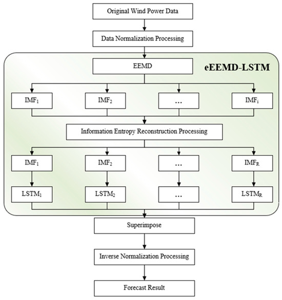
Figure 3.
The flowchart of the eEEMD-LSTM method.
4. Experiment and Result Analysis
To verify the performance of these methods, the efficiency and precision of eEEMD-LSTM are compared with other classical models. This chapter mainly includes the data selection processing and the wind power forecast performance chart contrast analysis.
4.1. Data Preprocessing
4.1.1. Data Selection
This section focuses on the experimental data used in the study. Considering the climate of a specific location changes little in the span of several years, the wind characteristics are also similar in different years; we take the sampled wind power data (sampling period: 15 min, unit: MW) from 2017 to validate the proposed method.
To better test the prediction effectiveness of the proposed method, we use three datasets of actual wind power data from the same wind farm in different periods, which are drawn from different seasons in 2017. The first dataset (data 1) is taken from a total of 10,000 wind power raw data from February 3 to May 19, the second (data 2) is taken from a total of 10,000 wind power raw data from May 19 to August 31, and the third (data 3) is taken from a total of 10,000 wind power raw data from August 31 to December 12. The values of data 1, data 2, and data 3 do not overlap. For every dataset, the sample is obtained from a scrolling window with a window size of 12, i.e., using the past 12 actual wind power values to predict the next one with 15-min intervals. The training set accounts for 90%, and the test set accounts for 10%.
The three sets of original wind power data are shown in Figure 4.
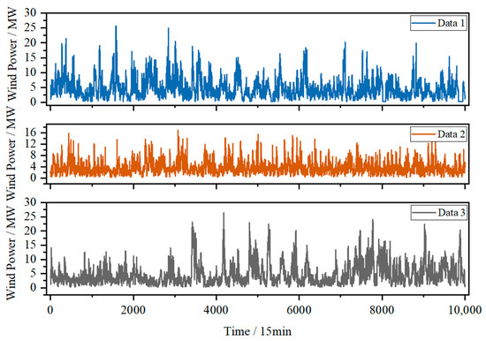
Figure 4.
Original wind power of data 1, data 2 and data 3.
To avoid problems caused by the order of magnitude of sample data, the maximum and minimum normalization method is adopted to normalize the data. The normalization formula is (2).
where xmin is the minimum value in the original data; xmax is the maximum value in the original data, and x is the original data.
4.1.2. Evaluation Metrics
Root mean square error (RMSE), also known as standard error, is a widely used evaluation metric which is very sensitive to small or significant errors in test data, as shown in Equation (3).
Mean absolute error (MAE) is the mean of absolute error, which can better reflect the actual situation of predicted error, as shown in Equation (4).
Mean absolute percentage error (MAPE) stands for mean absolute percentage error and is a relative measure that actually identifies the MAE scale as a unit of percentage rather than a unit of variable. MAPE is a relative error measure that uses absolute values to avoid positive and negative errors canceling each other out, as shown in Equation (5).
where PP,k is the forecasting value of wind power and PM,k is the true value of wind power.
4.2. Predictive Performance Analysis
To compare with other methods, we chose 12 prediction methods to test the same experimental data. Therefore, in this paper, we will analyze the event results in terms of two aspects: prediction efficiency and prediction performance.
4.2.1. Efficiency Analysis
In many experiments, it has been found that excessive IMF components have a significant impact on the efficiency of the ultra-short-term wind power prediction model, so eEEMD is used to reconstruct the data. Table 1 shows the figures obtained from IMF after EEMD and eEEMD processed the datasets.

Table 1.
The number of IMFs with EEMD and eEEMD.
Table 1 lists the number of IMFs obtained by applying EEMD and eEEMD to three datasets separately. The decomposed components of each dataset need to be predicted separately using a separate model. For the three sets of data currently used, the EEMD method decomposes each dataset into 12 components, and it is time-consuming to predict each component separately for the final reconstruction results. This method greatly affects the efficiency of wind power prediction. In this regard, we consider the eEEMD method for the reconstruction. Figure 5 shows the decomposition outcomes of dataset 1, which is obtained by applying the EEMD and the eEEMD algorithms.
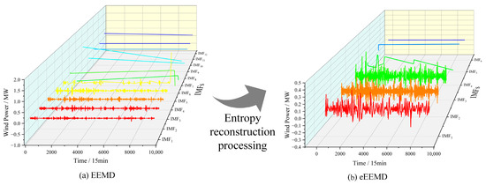
Figure 5.
Decomposition results of data 1. (a): EEMD; (b): eEEMD.
Figure 4 shows the distribution of a single IMFs using EEMD and eEEMD to decompose data 1. The comparison of the two decomposition methods for IMF fluctuation and decomposition shows that the eEEMD is a more effective data decomposition method. By reducing the number of IMFs and alleviating the endpoint problems in the decomposition process, eEEMD can extract time characteristics of data, thereby improving prediction efficiency. To compare the effects of EEMD and eEEMD on the prediction efficiency of the model more intuitively, the decomposition and reconstruction processes of the specific time required for two algorithms. Figure 6 shows the comparison results of the specific time required by the two algorithms. These findings indicate that eEEMD is a superior choice for data decomposition and prediction.
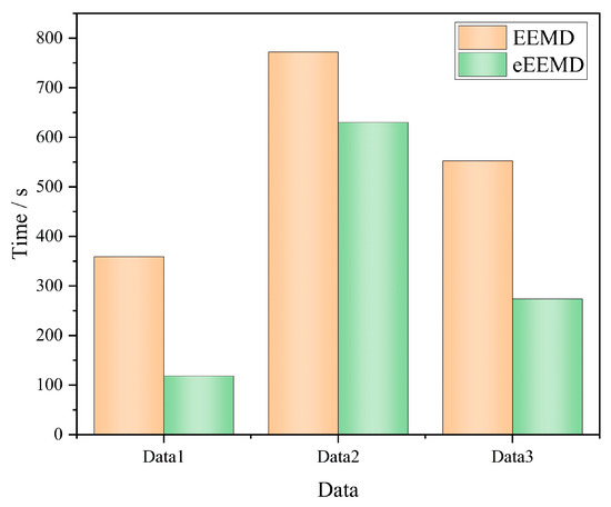
Figure 6.
Efficiency comparison of EEMD and eEEMD of data 1.
Figure 6 clearly shows that eEEMD can effectively improve the prediction efficiency of the model, and when the partial features of reconstruction are prominent. It can more significantly reduce the modeling time and improve the wind power prediction efficiency.
4.2.2. Accuracy Analysis
To compare the advantages and disadvantages of various prediction methods, we choose BR, SVR, gated recurrent unit (GRU), LSTM, EEMD-BR, EEMD-SVR, EEMD-GRU, EEMD-LSTM, eEEMD-BR, eEEMD-SVR, eEEMD-GRU, and eEEMD-LSTM to predict the same experimental data. In the experiment, the penalty coefficient is 1.0 of SVR. The parameters of the specific eEEMD-LSTM model are shown in Table 2.
Table 2.
Parameter settings.
GRU retains the necessary architecture of LSTM, which can control the forgetting factor and update the state unit simultaneously through a single gating unit, and dynamically control the time scale and forgetting behavior of different units in the network [22]. Too many comparison methods in the picture will affect the clarity. Therefore, the GRU, EEMD-GRU, and eEEMD-GRU methods no longer appear in the image analysis of the article and only the evaluation metrics result of the three methods are shown in Table 3.
Table 3.
Comparison of evaluation metrics.
To further compare the prediction performance of different methods, EEMD and eEEMD are combined with BR, SVR, and LSTM models separately, and 6 methods to predict wind power are obtained. Figure 7 shows the prediction error distribution of EEMD and eEEMD of the same model. The prediction error shown in Figure 7 is the absolute error of each data after the inverse normalization.
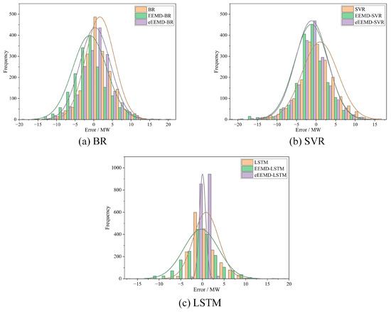
Figure 7.
Error distribution of different methods with different algorithms. (a): BR; (b): SVR; (c): LSTM.
Figure 7 shows the prediction error, which fluctuates around zero. The figure compares and analyzes the frequency distribution of prediction errors for various methods. In particular, Figure 7a compares BR, EEMD-BR, and eEEMD-BR methods, while Figure 7b,c compare the frequency distribution of prediction errors for SVR-related methods and LSTM-related methods, respectively.
It can be clearly seen from Figure 6 that regardless of which model is used, the model with EEMD can effectively reduce the error, and the frequency of error close to zero increases significantly. Furthermore, the error frequency of the eEEMD optimization algorithm is closest to zero. It is observed that the eEEMD-LSTM model has the highest error frequency near zero.
This phenomenon is attributed to the fact that the IMFs obtained from EEMD decomposition has more distinct time series characteristics than the original dataset. The combined model reduces the complexity of model prediction, and the prediction error is smaller than that of a single model. By combining differential training with reconstructed components, the combined use of eEEMD and model has been able to prove a significant improvement in reducing prediction errors. Our research findings indicate that differential training may alleviate the situation of under-learning or over-learning situation up to some extent. The eEEMD-LSTM model showed the most significant improvement in reducing prediction error, while the eEEMD-SVR showed the least improvement. This observation indicates that the effectiveness of optimization algorithm has limited benefit in improving the prediction performance of different methods. However, the entire pair is still effective in improving the prediction results.
To further analyze the forecast trend of the 9 methods, the predicted value of each model is compared with the actual value. The overall forecast trend of 9 methods in data 1 is shown in Figure 8, and the partly forecast trend is shown in Figure 9.
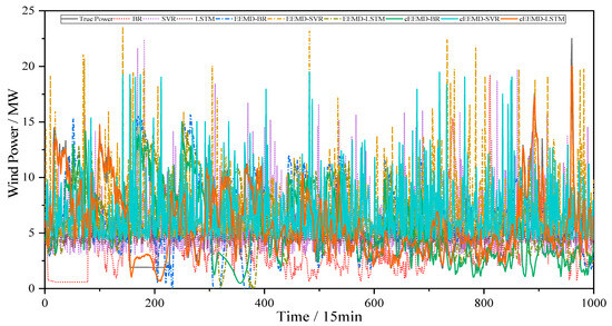
Figure 8.
Prediction effect of different methods for data 1.
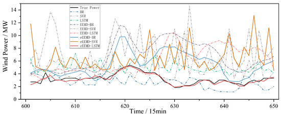
Figure 9.
Partial prediction effect of different methods for data 1.
The results of Figure 8 and Figure 9 indicate that the prediction performance of a single model is relatively poor. Among various methods, the fitting curve of the BR model has a large deviation, while the fitting effect of the LSTM model is better. Although the EEMD decomposition algorithm improves the predictive performance of a single model, the overall prediction effect is still not ideal. The combination of the eEEMD method and the model effectively improves the prediction effect, and the improvement effect is more obvious than EEMD. The eEEMD method is implemented in all methods, and the prediction effect results show that the eEEMD-LSTM has the best prediction effect. Additionally, Figure 8 and Figure 9 show the prediction trends for the 9 methods, which are consistent with the overall error variation shown in Figure 7.
The experimental results in Table 3 were calculated using RMSE, MAE, and MAPE. The smaller the calculation result, the better the prediction effect of this method. The evaluation metrics calculation results are the normalized results of the data.
Table 3 mainly compares the differences of different evaluation metrics of BR, SVR, GRU, and LSTM in 3 sets of data when EEMD and eEEMD are used respectively. Table 3 shows that the independent BR model has the weakest prediction performance, while LSTM surpasses all models in effectiveness of all models.
Regarding the RMSE evaluation metrics, EEMD-BR increased by 57.9% at most, while EEMD-SVR increased by 15.7% on average, and EEMD-LSTM increased by at least 15.1%. The MAE evaluation metrics show that EEMD-BR has increased by 58.2% at the maximum, EEMD-SVR by 15.2% on average, EEMD-GRU by 21.28% on average, and EEMD-LSTM by at least 21.7%. Finally, the MAPE evaluation metrics show EEMD-BR increasing by a maximum of 67.4%, EEMD-SVR by an average of 83.6%, and EEMD-LSTM by at least 23.0%.
When the methods are decomposed by eEEMD, the eEEMD-SVR model showed the most stable improvement in prediction effectiveness, while the eEEMD-LSTM model shows the best overall prediction results. Furthermore, when the eEEMD method is used for reconstruction, eEEMD-LSTM produces the best overall prediction results, while eEEMD-BR shows the most significant improvement.
Considering the RMSE evaluation metrics, the increase rate of eEEMD-BR is at least 18.6%, and the maximum increase rate of eEEMD-LSTM is 34.2%. For the MAE evaluation metrics, eEEMD-BR increased by at least 17.9%, eEEMD-SVR by 6.8% on average, and eEEMD-LSTM by 22.6% at the maximum. Finally, the MAPE evaluation metrics show eEEMD-BR increasing by at least 1.3%, eEEMD-SVR by an average of 83.6%, eEEMD-GRU increased by 1.72% and eEEMD-LSTM by 52.1% at the maximum.
The predictive performance of the method not only focuses on the numerical results of one of the evaluation indicators, but also requires analysis from multiple perspectives. The proposed method eEEMD-LSTM is not very efficient on MAPE evaluation metrics of data 1 and data 3, but is still superior to most models. Except for the MAPE evaluation metrics, the eEEMD-LSTM method is better than other models in other metrics. By analyzing the prediction results of different models, it can be concluded that this method has a better prediction performance than other methods.
To more clearly compare the evaluation indicators of different methods, the specific values are visualized. The error comparison of different methods is shown in Figure 10 below.
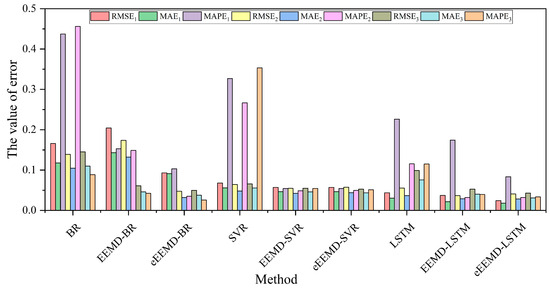
Figure 10.
Error comparison of different methods.
The histograms for the relevant evaluation metrics are shown in Figure 10. In particular, the red column depicts the RMSE1 of nine methods, including BR, EEMD-BR, eEEMD-BR, SVR, EEMD-SVR, eEEMD-SVR, LSTM, EEMD-LSTM, and eEEMD-LSTM, with data 1. Similarly, the green MAE1 and purple columns MAPE1 indicate the MAE and MAPE of each model with data 1, respectively. The yellow columns RMSE2, blue columns MAE2, and pink columns MAPE2 show the relevant evaluation with data 2, while the dark green columns RMSE3, cyan columns MAE3, and orange columns MAPE3 represent the relevant evaluation with data 3. Based on Figure 10, the eEEMD-LSTM, as described in the present study, exhibited the minimum evaluation error, irrespective of the evaluation standard employed.
5. Conclusions
Accurately predicting wind power is a key aspect of the development of wind power generation. However, the ability to efficiently predict wind power is hindered when dealing with a large amount of data related to EEMD decomposition and training different sub-components. To address these issues, we propose a new ultra-short-term wind power prediction method using eEEMD-LSTM. Among them, the LSTM model is suitable for the prediction of complex time series and has good generalization performance. eEEMD can solve the problem of excessive sequence components, thereby improving the efficiency of ultra-short-term wind power prediction. The eEEMD method has better generalization performance, shorter off-line training time, and higher efficiency. The methods proposed in this article include data selection, eEEMD decomposition and reconstruction, eEEMD-LSTM prediction, differential training error target setting, and comparative analysis of different methods. The experimental results show that LSTM has better fitting and prediction performance than BR, SVR, and GRU when dealing with the same data complexity. Compared with EEMD, the eEEMD method can effectively improve prediction efficiency. In addition, the analysis of wind power data at the same time by different methods shows that the eEEMD-LSTM network can improve the accuracy of wind power prediction and perform well in ultra-short-term wind power prediction of complex time series. However, under extreme working conditions, it is relatively weak to suppress possible over-learning or under-learning by adjusting the training error of the model through differentiation, so it is urgent to improve the differentiation degree of the sub-model. Therefore, adjusting other parameters of the model based on data differences, and this measure will help to further improve the prediction performance of the model.
Author Contributions
Conceptualization, J.H.; Formal analysis, W.Z. and J.Q.; Investigation, S.S.; Methodology, J.H.; Software, W.Z.; Supervision, S.S.; Writing—original draft, W.Z.; Writing—review & editing, J.H., W.Z. and J.Q. All authors have read and agreed to the published version of the manuscript.
Funding
This research was funded by the National Nature Science Foundation of China, grant number U1504617.
Data Availability Statement
The data used in this work are from the publicly archived datasets on Kaggle and are available at https://www.kaggle.com/berkerisen/wind-turbine-scada-dataset, accessed on 17 October 2022.
Conflicts of Interest
The authors declare no conflicts of interest.
References
- International Energy Agency. World Energy Outlook 2023. Available online: https://www.iea.org/reports/world-energy-outlook-2023 (accessed on 30 October 2023).
- Nadeem, F.; Aftab, M.A.; Hussain, S.M.S.; Ali, I.; Tiwari, P.K.; Goswami, A.K.; Ustun, T.S. Virtual Power Plant Management in Smart Grids with XMPP Based IEC 61850 Communication. Energies 2019, 12, 2398. [Google Scholar] [CrossRef]
- Veers, P.; Dykes, K.; Lantz, E.; Barth, S.; Bottasso, C.L.; Carlson, O.; Clifton, A.; Green, J.; Green, P.; Holttinen, H.; et al. Grand Challenges in the Science of Wind Energy. Science 2019, 366, eaau2027. [Google Scholar] [CrossRef] [PubMed]
- Hoyos-Santillan, J.; Miranda, A.; Lara, A.; Rojas, M.; Sepulveda-Jauregui, A. Protecting Patagonian Peatlands in Chile. Science 2019, 366, 1207–1208. [Google Scholar] [CrossRef]
- Xing, Y.; Chen, Y.; Huang, S.; Wang, P.; Xiang, Y. Research on Dam Deformation Prediction Model Based on Optimized SVM. Processes 2022, 10, 1842. [Google Scholar] [CrossRef]
- Shan, Y.; Chen, S.; Zhong, Q. Rapid Prediction of Landslide Dam Stability Using the Logistic Regression Method. Landslides 2020, 17, 2931–2956. [Google Scholar] [CrossRef]
- Lin, Z.; Liu, X.; Collu, M. Wind Power Prediction Based on High-Frequency SCADA Data along with Isolation Forest and Deep Learning Neural Networks. Int. J. Electr. Power Energy Syst. 2020, 118, 105835. [Google Scholar] [CrossRef]
- Chen, X.; Zhang, X.; Dong, M.; Huang, L.; Guo, Y.; He, S. Deep Learning-Based Prediction of Wind Power for Multi-Turbines in a Wind Farm. Front. Energy Res. 2021, 9, 723775. [Google Scholar] [CrossRef]
- Gu, B.; Zhang, T.; Meng, H.; Zhang, J. Short-Term Forecasting and Uncertainty Analysis of Wind Power Based on Long Short-Term Memory, Cloud Model and Non-Parametric Kernel Density Estimation. Renew. Energy 2021, 164, 687–708. [Google Scholar] [CrossRef]
- Han, L.; Jing, H.; Zhang, R.; Gao, Z. Wind Power Forecast Based on Improved Long Short Term Memory Network. Energy 2019, 189, 116300. [Google Scholar] [CrossRef]
- Huang, J.; Li, C.; Huang, Z.; Liu, P.X. A Decomposition-Based Approximate Entropy Cooperation Long Short-Term Memory Ensemble Model for Short-Term Load Forecasting. Electr. Eng. 2022, 104, 1515–1525. [Google Scholar] [CrossRef]
- Shahid, F.; Zameer, A.; Muneeb, M. A Novel Genetic LSTM Model for Wind Power Forecast. Energy 2021, 223, 120069. [Google Scholar] [CrossRef]
- Yang, H.; Jiang, Z.; Lu, H. A Hybrid Wind Speed Forecasting System Based on a ‘Decomposition and Ensemble’ Strategy and Fuzzy Time Series. Energies 2017, 10, 1422. [Google Scholar] [CrossRef]
- Zhao, N.; Li, R. EMD Method Applied to Identification of Logging Sequence Strata. Acta Geophys. 2015, 63, 1256–1275. [Google Scholar] [CrossRef][Green Version]
- Ambark, A.S.A.; Ismail, M.T.; Al-Jawarneh, A.S.; Karim, S.A.A. Elastic Net Penalized Quantile Regression Model and Empirical Mode Decomposition for Improving the Accuracy of the Model Selection. IEEE Access 2023, 11, 26152–26162. [Google Scholar] [CrossRef]
- Michelson, E.A.; Cohen, L.; Dankner, R.E.; Kulczycki, A.; Kulczycki, A. Eosinophilia and Pulmonary Dysfunction during Cuprophan Hemodialysis. Kidney Int. 1983, 24, 246–249. [Google Scholar] [CrossRef] [PubMed]
- Wang, J.; Du, G.; Zhu, Z.; Shen, C.; He, Q. Fault Diagnosis of Rotating Machines Based on the EMD Manifold. Mech. Syst. Signal Process. 2020, 135, 106443. [Google Scholar] [CrossRef]
- Yang, Y.; Yang, Y. Hybrid Method for Short-Term Time Series Forecasting Based on EEMD. IEEE Access 2020, 8, 61915–61928. [Google Scholar] [CrossRef]
- Zhang, G.; Zhou, H.; Wang, C.; Xue, H.; Wang, J.; Wan, H. Forecasting Time Series Albedo Using NARnet Based on EEMD Decomposition. IEEE Trans. Geosci. Remote Sens. 2020, 58, 3544–3557. [Google Scholar] [CrossRef]
- Meng, A.; Chen, S.; Ou, Z.; Ding, W.; Zhou, H.; Fan, J.; Yin, H. A Hybrid Deep Learning Architecture for Wind Power Prediction Based on Bi-Attention Mechanism and Crisscross Optimization. Energy 2022, 238, 121795. [Google Scholar] [CrossRef]
- Huang, J.; Niu, G.; Guan, H.; Song, S. Ultra-Short-Term Wind Power Prediction Based on LSTM with Loss Shrinkage Adam. Energies 2023, 16, 3789. [Google Scholar] [CrossRef]
- Cho, K.; van Merrienboer, B.; Bahdanau, D.; Bengio, Y. On the Properties of Neural Machine Translation: Encoder–Decoder Approaches. In Proceedings of the 8th Workshop on Syntax, Semantics and Structure in Statistical Translation, SSST 2014, Doha, Qatar, 25 October 2014; Association for Computational Linguistics (ACL): Doha, Qatar, 2014; pp. 103–111. [Google Scholar]
Disclaimer/Publisher’s Note: The statements, opinions and data contained in all publications are solely those of the individual author(s) and contributor(s) and not of MDPI and/or the editor(s). MDPI and/or the editor(s) disclaim responsibility for any injury to people or property resulting from any ideas, methods, instructions or products referred to in the content. |
© 2024 by the authors. Licensee MDPI, Basel, Switzerland. This article is an open access article distributed under the terms and conditions of the Creative Commons Attribution (CC BY) license (https://creativecommons.org/licenses/by/4.0/).