Improving Computation Time for Optimization Runs of Modelica-Based Energy Systems

Abstract

Mathematical optimization is a widespread method in order to improve, for instance, the efficiency of energy systems. A simulation approach based on partial differential equations can typically not be formulated as an optimization problem, thus requiring interfacing to an external optimization environment. This is, among others, also true for the programming language Modelica. Because of high computation time, such coupled approaches are often limited to small-scale optimization problems. Since simulation models tend to get more complex, simulation time and, in turn, associated optimization time rise significantly. To enable proper sampling of the search space, individual optimization runs need to be solved in acceptable times. This paper addresses the search for a proper optimization approach and tool to couple with Modelica/Dymola. The optimization is carried out on an exemplary power plant model from the ClaRa-Library using an evolutionary algorithm (SPEA2-based) with Ansys optiSlang. To verify and evaluate the results, a comparison with the standard Dymola optimization library is performed. Both parallelization and indirect optimization with surrogate models achieved a significant runtime reduction by a factor of up to 5.4. The use of meta models is particularly advantageous for repetitive optimization runs of the same optimization problem but may lead to deviations due to the calculated approximations.

1. Introduction

Process modeling and simulation is becoming increasingly important to achieve improvements in today’s complex energy systems and technologies [1]. The model formulation can be carried out via several programming languages. A frequently used language is the object- and equation-oriented programming language Modelica, which is particularly suitable for the representation of dynamic processes [2,3]. To improve the handling of the modeling process, simulation environments such as Dymola are usually used [4]. Based on these models, extensive investigations such as design or control optimizations can be performed. A widely used method is the parameter variation, which is quite simple to perform but becomes more time-consuming as the complexity of the model increases. In these cases, mathematic optimization is used instead. Therefore, an optimization problem has to be defined and solved with the help of algorithms. The programming language Modelica, which is designed for simulation tasks, does not allow for the formulation of such optimization problems. Thus, a coupling with external optimization languages or optimization environments is necessary [2]. In the field of energy systems, a wide variety of such environments have already been used for coupling with Dymola (see Section 3). This paper presents the first-time coupling of Dymola 2021x and Ansys optiSLang 2022 R1 [5] in order to solve static optimization problems. For this purpose, the implemented workflow and its main features as well as the used algorithm are presented in Section 4 and Section 5. The verification of the results is finally achieved by a comparison with the standard Dymola optimization library (DLR Optimization Library [6]). This library offers a wide range of different optimization techniques that are easy to apply. However, a huge disadvantage is the required runtime for optimization, which will be further discussed in Section 6. For a better understanding of the results, relevant basics of mathematical optimization are presented first.

2. Mathematical Optimization

The first step when dealing with optimization is the definition of the problem itself. Therefore, the objective function $f\left(x\right)$, the optimization variable $x$ and possible restrictions must be defined [7,8]. For this study, we split optimization into the static and transient type, depending on the contents of the optimization variable. A typical application for static optimization is design optimization, where an optimal design of a component is determined disregarding transient features [9,10]. Transient optimization is, for instance, used to calculate optimal process control strategies [11].

When choosing the appropriate algorithm, the specific properties of the algorithm as well as the specifications of the optimization problem must be considered [9,12]. In application-related problems, multi-objective optimization tasks are the most common. In contrast to the single-objective optimization, several objective functions are optimized simultaneously. Usually, these functions are in conflict with each other. 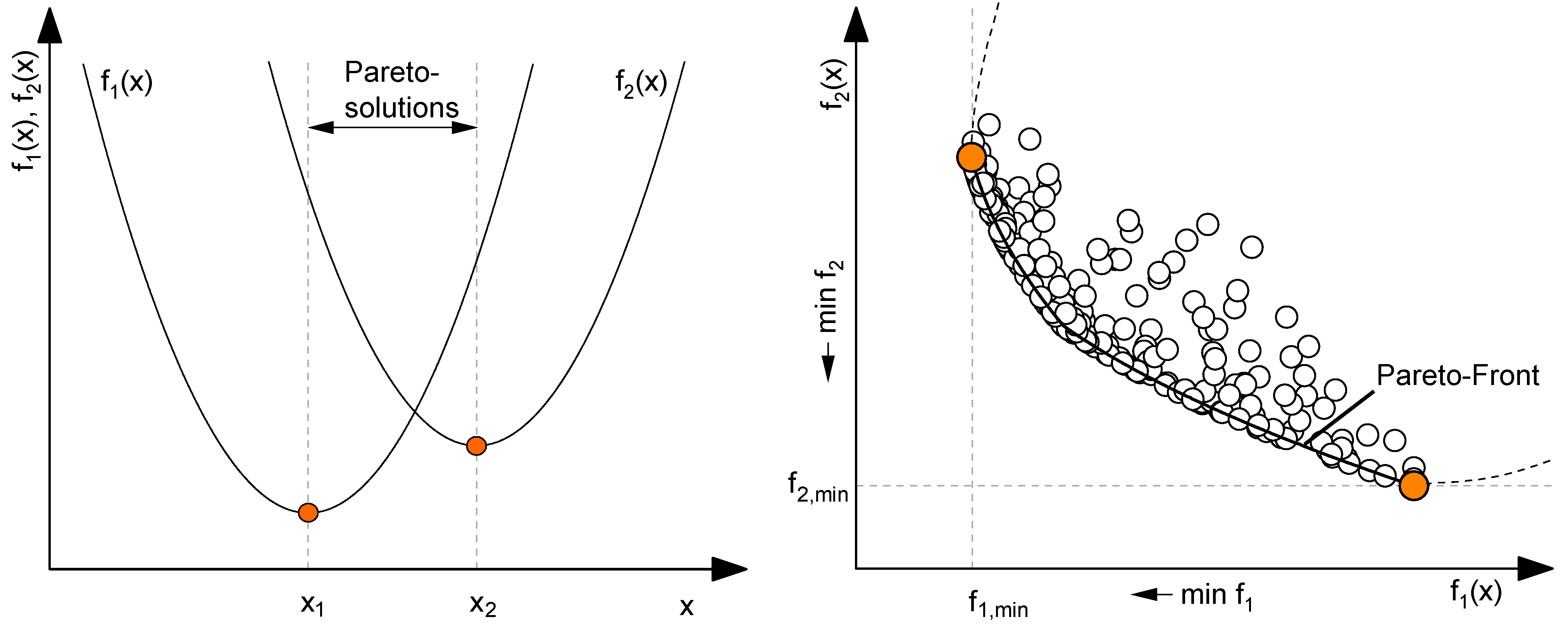As a result, there is no solution where both objective functions reach their individual optimum [9,13,14,15]. This context can be described by the so-called Pareto front (see Figure 1). Illustrated are the two fictitious objective functions $f_1\left(x\right)$ and $f_2\left(x\right)$, which are to be minimized by a variation of $x$. By using the single optima ($x_1$ and $x_2$), three characteristic ranges can be identified. Whereas an increase of $x$ in the range $x<x_1$ leads to an improvement of both functions, an increase for $x>x_2$ causes a deterioration of both functions. The relevant range is thus located between the two individual optima ($x_1<x<x_2$). Within this range, an improvement of one objective function can only be realized by a deterioration of the other criterion. This means that there is no longer a single optimum, as in the case of the single-objective optimization. Instead, there is a set of different optima, also called the Pareto-optimal set or Pareto solutions. By comparing the two objective functions, this set can be represented as a subset of the boundary curve (Pareto front on the right). By selecting a weighting, a problem-specific overall solution can then be determined [9,13,14,15].

3. Optimization with Dymola

In the area of energy systems, various couplings between Dymola and different optimization environments have already been implemented. The choice of the appropriate environment is problem-specific and depends primarily on the type of optimization problem.

Table 1. Couplings of Dymola and optimization environments in the field of energy systems.

Model	Method	Optimization-Tool	Ref.
Chilled water plant	Real-time optimization	DLR Optimization Library	[16]
CO2 heat pump and thermal storage	Optimal control	DLR Optimization Library	[17]
Osmosis hybrid system	Design optimization	DLR Optimization Library	[18]
Hybrid energy systems (HES)	Optimal control	Matlab	[19]
Decentralized energy supply	Optimal control	Simulink	[20]
Thermal management system	Optimal control	MUSCOD-II	[21]
Chiller plant	Optimal control	Matlab	[22]
Heat pump	Design optimization	OMOptim	[23]
Combined heat and power plant (CHP)	Optimal control	GenOpt	[24]
Central cooling plant	Optimal control	GenOpt	[26]
Chiller plant	Optimal control	GenOpt	[25]
Chilled water system	System configuration	GenOpt	[27]
Discontinuously models	Sensitivity analysis	Fisemo	[28]

shows an overview of published investigations and lists the used optimization tool. The DLR Optimization Library is fully integrated in Dymola and can be used to define multicriteria and trajectory optimization problems. In the three listed examples [16,17,18], different types of models and optimization problems were investigated. Dymola is currently one of over 170 tools that support the FMI standard. It allows for the export and exchange of simulation models into other simulation or optimization environments. Studies [19,20,21] are using this standard for an optimization in Matlab and Simulink with the focus on optimal control. In the study in [22], Matlab is used as an optimization platform. Instead of FMI, an optimization workflow is presented. The workflow uses a Dymola script to run the simulation with different input parameters. The results are imported into Matlab from result files (dsres.mat) using pre-implemented functions. The study in [23] uses the optimization environments of OMOptim and Dymola as a simulation tool. To access the model structure and adapt the input variables, OpenModelica is used. In the shown example, a design optimization of a heat pump is presented. The optimization program GenOpt is a text-based system that uses the input and output files of a simulation software to perform the optimization. The studies in [24,25,26] present an optimal control problem, and [27] solves a design optimization with GenOpt. Pfeiffer [28] utilizes the FISEMO environment to perform a numerical sensitivity analysis of Modelica models. Dymola is used for the modeling process and the export of the model into C-Code. Integration into the FISEMO environment is achieved using the DASPK3.1 package.

Most of the listed publications deal with transient optimization and focus on optimal control problems. The static optimization is less frequent and only addressed in two publications with small-scale problems. In order to test the optimization framework optiSLang and contribute to the landscape of investigations of static optimization-simulation coupling, a proof of concept with a model of a coal-fired power plant is set up and carried out in this paper. One of the main advantages of optiSLang is the support for high-order parameter spaces, and thus extensive sensitivity analysis as well as comparatively complex design optimization calculations. In the field of mechanical construction, for instance, optimization problems with up to 30,000 independent variables were solved [29]. Since there is currently no direct connection to Dymola, a workflow will be presented in the first step (Section 4). Solving dynamic optimization problems with optiSLang is possible as well but will not be further discussed within this paper.

4. Coupling of Dymola and Ansys optiSLang

Since there is not yet a direct coupling option for Dymola and optiSLang, an appropriate workflow had to be developed. The implemented workflow presented in this paper enables an automatic data exchange between Dymola and optiSLang (see Figure 2). optiSLang works according to the principle of variance calculation, which is why several model simulations and modifications of the model have to be performed [5]. Therefore, a text-based solver chain is implemented within the optiSLang environment.

Dymola is used for the modeling process of the respective system in the programming language Modelica. The model can then be translated into C-Code and saved as an executable file with an associated input file. The input file contains essential initial values, model parameters and simulation settings that are needed for the simulation run of the model. After a successful simulation, the results are saved into output files. By modifying the input file, different model parametrizations, and therefore results, can be generated.

optiSlang uses these three files to perform the optimization. As a first step, the optimization problem must be defined in the optiSLang environment. In contrast to the original mathematical optimization, it is not necessary to develop a complex mathematical objective function. Instead, the optimization is performed using a black box model of the Dymola model (executable file). The input variables are set as optimization variables, and the output variables are set as target criteria. The optimization variables (tuners) must be extracted from the input file. For each evaluation of the algorithm, one modified input file is created. Each of these files has different tuning values, which are varied in a defined range in order to achieve the optimum. The validation of the optimum is achieved using target criteria, which are integrated in the model and calculated through a simulation (via batch script). The results of each simulation are saved into individual output files. optiSLang extracts these values and evaluates them according to the chosen algorithm.

Although the black box model simplifies the definition of the optimization problem, it also means that there is no knowledge of the mathematical structure of the problem. However, this knowledge is usually necessary for the choice of a suitable algorithm. To counteract this problem, optiSLang offers the user a traffic light system that recommends an algorithm based on the determined internal optimization problem (number of inputs, single- or multi-objective problem, etc.). It must be taken into account that this recommendation depends on the mathematical solvability of the problem and does not guarantee the best possible result. Thus, it is still necessary to know about the functionality of the individual algorithms to select a suitable one for a given optimization problem.

5. Case Study: Coal-Fired Power Plant

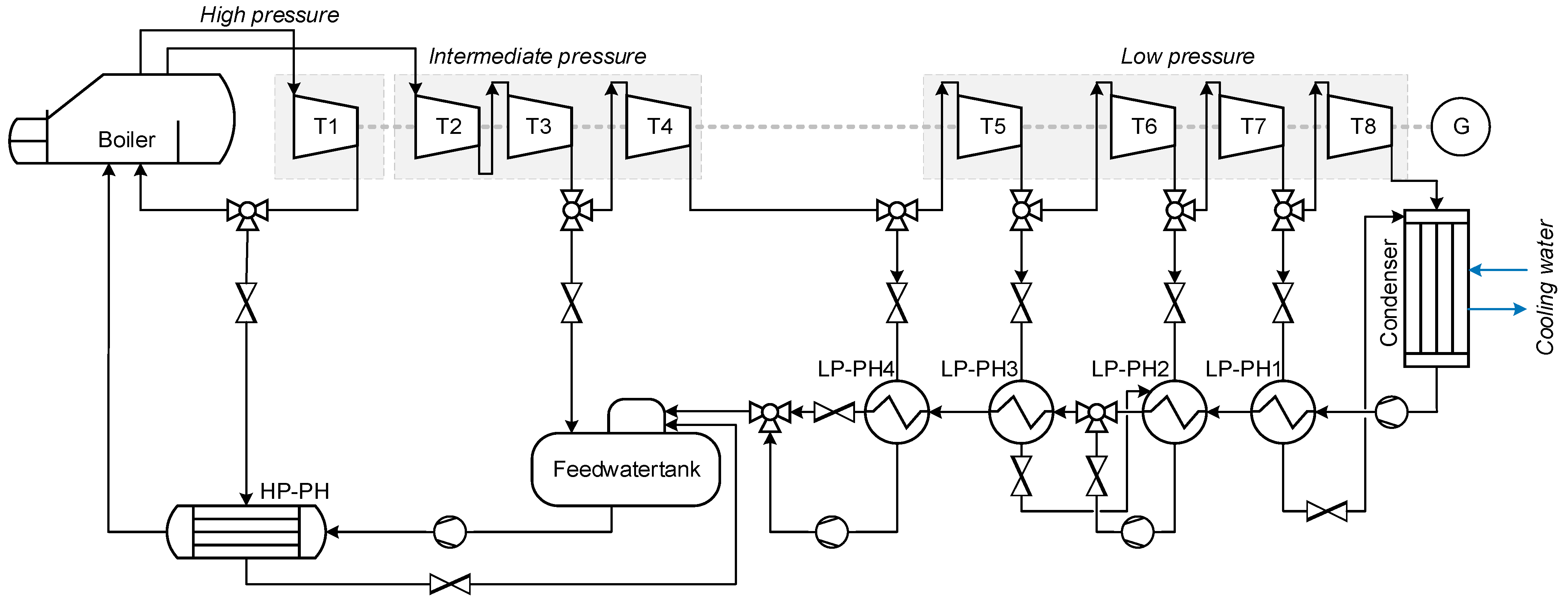
In order to validate the implemented workflow, an optimization run is performed using an example model of the open-source library ClaRa [30]. The chosen model represents a coal-fired power plant with eight turbine stages including feed water preheating. Figure 3 shows a simplified schematic of the plant. After passing the boiler, the generated steam flows through the individual turbine stages until it is expanded to the condenser pressure. The collected condensate is then preheated by the four low-pressure preheaters (LP-PH) before it enters the steam-heated feed water tank. The feed water is preheated by the high-pressure preheater (HP-PH) before it enters the boiler. The power plant is designed to provide 580 MW_el. In the simulation scenario, two load reductions to 70 percent load are performed. One simulation run of 10,000 s requires around 118 s simulation time.

The optimization is carried out using the HP preheater as an example component due to its huge impact on the preheating section. The HP-PH model is a shell-and-tube heat exchanger for which selected tube parameters are to be optimized. Adjusting the geometry data influences the heat transfer surface and the pressure losses in the heat exchanger. This results in deviating mass flow rates and temperatures in the entire power plant. This particularly affects the heating requirements of the feed water tank and HP-PH, as well as the mass flow rates of the high-pressure, medium-pressure and low-pressure turbine stages. The individual effects can vary depending on the selected geometry and therefore lead to different overall effects, which are not described in detail in this paper. Further information about the model can be obtained from the open-source library ClaRa [30].

The aim of the optimization is the improvement of the overall power plant efficiency with respect to the investment costs of the heat exchanger. Therefore, inner tube diameter $d_i$, outer tube diameter $d_o$ and tube length $l$ are to be optimized (Equation (1)). The resulting multi-objective optimization problem is shown below. In many cases, optimization tools simplify a multi-objective problem to a single-objective problem by combining the multiple functions into a single sum function with individual weights or by focusing on one function and introducing the remaining as constraints [31]. However, optiSLang instead uses an interactive method (see Section 2), which allows for dealing with several functions simultaneously. The resulting Pareto front can be used to identify the area of interest, where focused optimization runs can be performed.

A simple degression function is implemented for estimating the investment costs (see Equation (2)) [32,33]. Therefore, the heat transfer surface is set in relation to a theoretical reference heat exchanger ($A_{ref}$ = 1500 m² and $K_{i,ref}$ = 800,000 €) and is simplified by Equation (3). The degression exponent n was set to 0.6 [32,33]. The price index effect from $PI$ and ${PI}_{ref}$ is neglected in this example. The efficiency is automatically calculated within in the model and is equal to the outlet power and inlet power ratio (see Equation (4)). The negative equation sign is used to transform the maximization problem into a minimization problem.

Table 2. Specifications of the optimization variables $d_i$, $d_o$ and $l$.

Tuner	Lower Boundary (m)	Initial Value (m)	Upper Boundary (m)
di	0.015	0.020	0.024
do	0.025	0.028	0.031
l	9	10	11

shows the individual limits of the tuner variables. The initial values of the overall system efficiency ${\eta }_{ref}$ and the investment costs $K_{i,ref}$ are 51.58% and EUR 802,545.

$$x={(d_o,d_i,l)}^T$$

(1)

$$\min f_1\left(x\right)=K_{i,ref}\cdot {\left(\frac{A\left(x\right)}{A_{ref}}\right)}^n\cdot \left(\frac{PI}{{PI}_{ref}}\right)$$

(2)

$$A(x)=2\pi \cdot \frac{d_o+d_i}{2}\cdot l\cdot n_T$$

(3)

$$\min f_2=-P_{out}/P_{in}$$

(4)

Optimization Algorithm

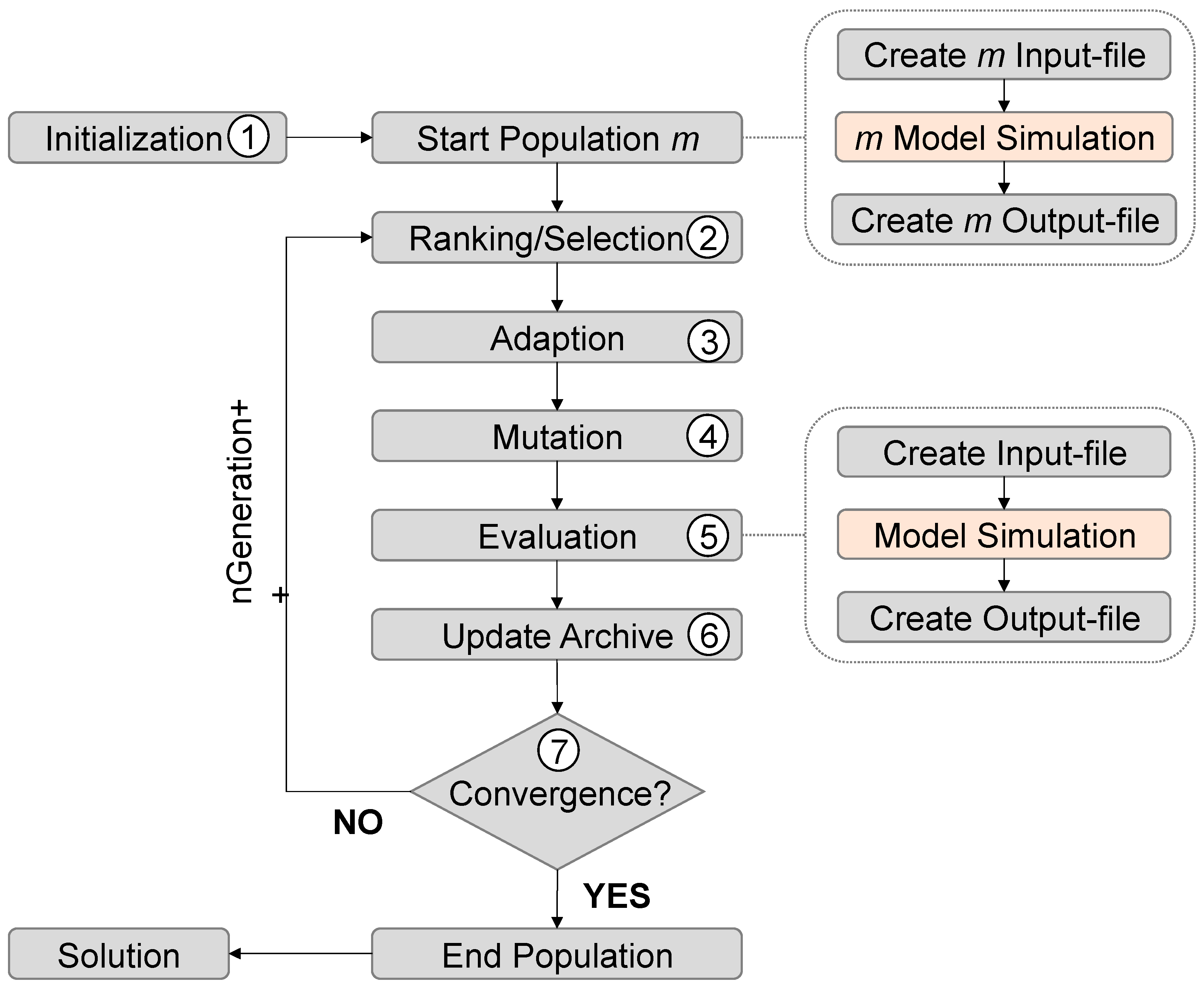
As a solving algorithm, a modified implementation of the Strength Pareto Evolutionary Algorithm 2 (SPEA2 [34]) is used. Figure 4 shows the general flowchart of the algorithm and indicates the interaction with the implemented workflow from Section 4.

After initialization of the simulation model, a start population of the size m is generated (Step 1). Therefore, m modified input files are created, and m respective simulation runs are performed. A dominance-based ranking system is used to assign a corresponding fitness value to each solution, which are extracted from the m output files (Step 2). The iteration loop starts after the assignment process is done by using adaption (e.g., crossover or swarm movement) and mutation methods. The additional designs must be evaluated and ranked once more (Step 5). Therefore, new model simulations are required. Beneficial solutions are used to update the archive (containment for good solutions) and checked for convergence (Step 7). If the convergence criteria are reached, the optimization terminates, and the end population is stated. In the negative case, steps 2 to 7 are repeated until convergence or a termination criterion are reached. Since each evaluation requires one simulation of the model, optimization runtime is highly affected by simulation runtime and the number of total simulations. For a time-efficient optimization, both should be reduced as far as possible.

The described steps can be modified further by changing the algorithm parameter (e.g., mutation rate or crossover method). This allows the user to adapt the algorithm to the specific problem. The optimization runs presented in this paper use the optiSLang standard settings. All calculations are carried out under Windows 10 on an Intel Core i5-6500 (3.2 GHz processor) with 8 GB RAM.

6. Results

6.1. Direct and Indirect Optimization

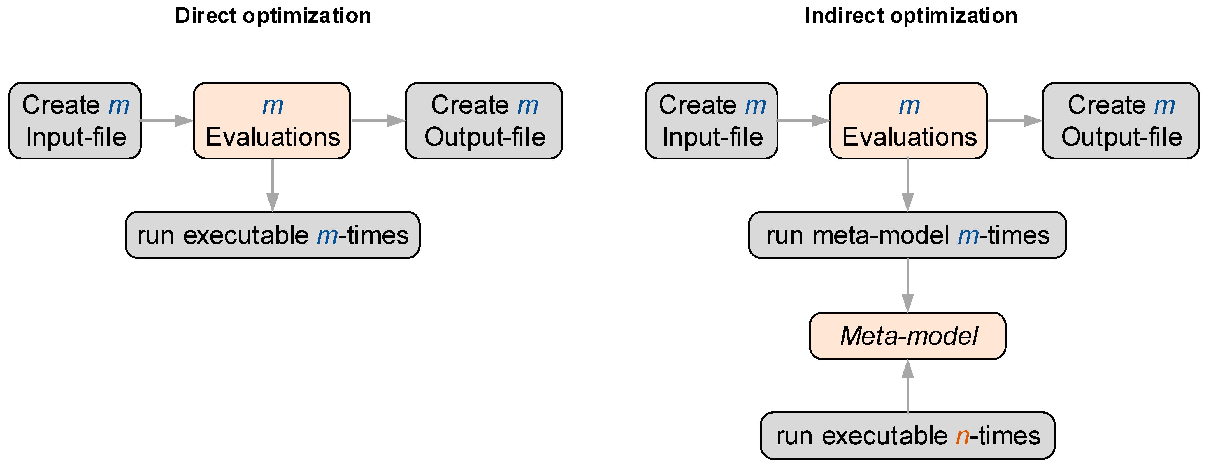
The optimization can be achieved as a direct or indirect optimization (Figure 5). In the case of the direct optimization, an individual model simulation is carried out for each evaluation of the algorithm. The indirect optimization, on the other hand, uses a surrogate model (meta model) of the simulation model. The meta model is determined based on n model simulations (100 by default) via a sensitivity analysis (SA). The SA provides several response surfaces that mathematically describe the correlation between the target criteria and the chosen optimization variables. Both variants have individual advantages and disadvantages that are described in more detail below.

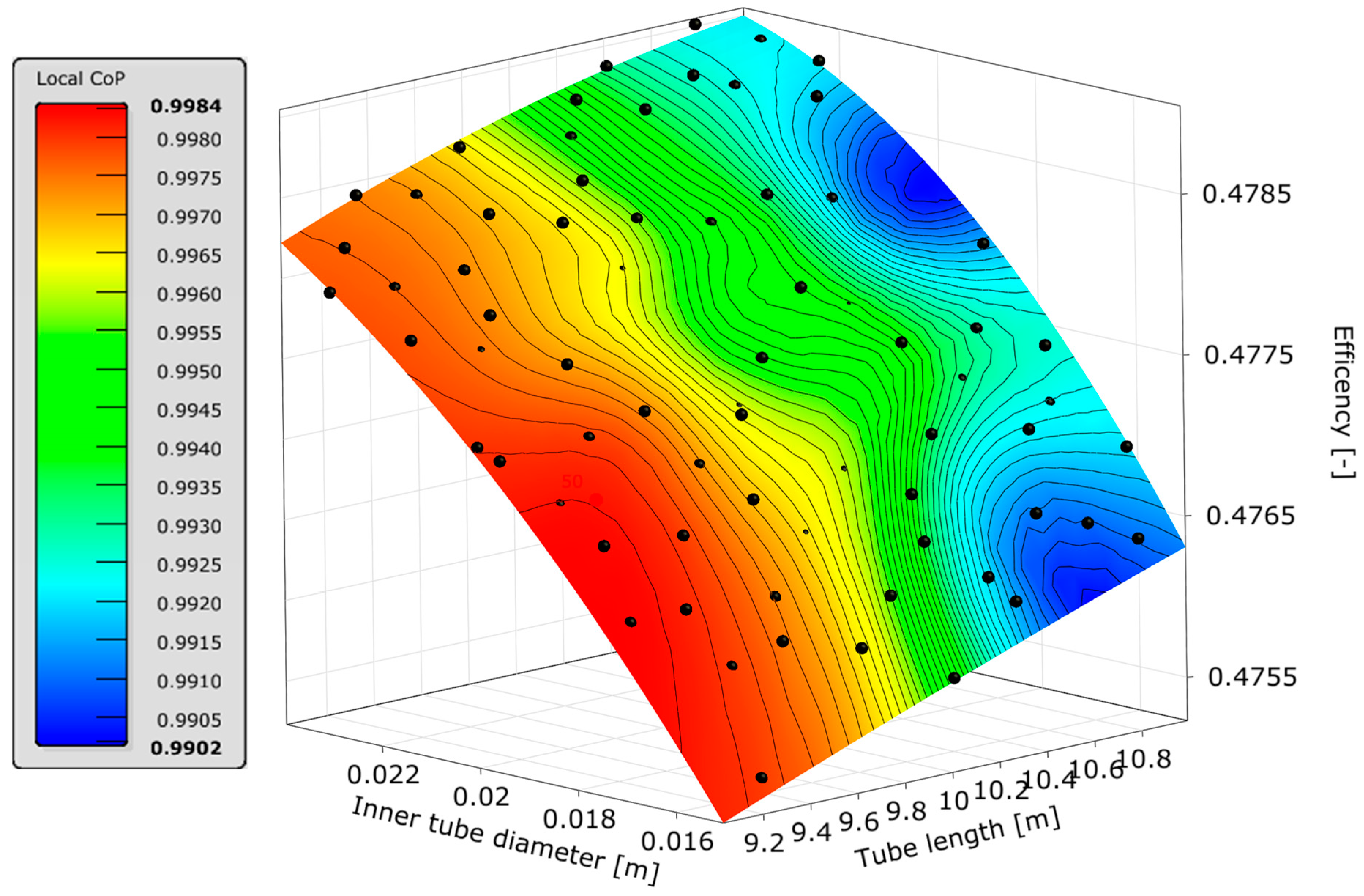
Figure 6 shows an example response surface of the overall system efficiency and its correlation to the tube length and the inner tube diameter of the HP-PH. For the approximation, a combination of several approximation techniques such as Kriging or neuronal networks are used. In this case, the color scale indicates the local forecast quality of the approximation. Therefore, the so-called Coefficient of Prognosis (COP) is used. This value is a validation criterion developed by optiSLang to describe the quality of the approximation. It is calculated using a cross-validation procedure [5]. In this case, the COP is on a very high level across the entire surface. In systems with more complex and discontinuous process behavior, lower COP values are generally reached. In such cases, it is possible to use other Design of Experiment (DoE) methods and/or to increase the number of samples (n). Another feature of the SA is the filtering of non-relevant parameters to simplify the optimization problem.

6.2. Runtime Comparison of Direct and Indirect Optimization

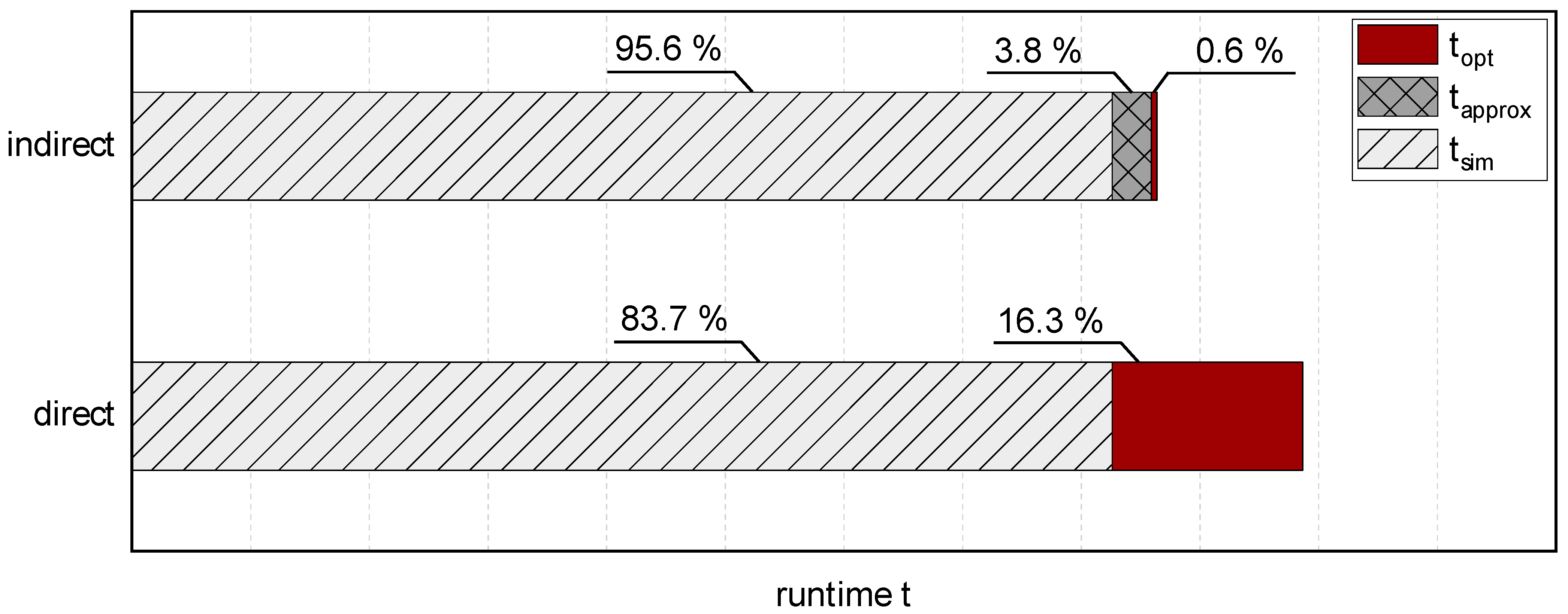
A comparison of the direct and indirect optimization methods indicates a time advantage in favor of the indirect method. Both calculations are carried out with the same number of model simulations and algorithm evaluations. For the comparison, the overall runtime ($t_{dir}$ and $t_{indir}$) is further separated into different categories (see Equations (5) and (6)). Hereby, a more detailed understanding of the optimization processes is achieved. The different categories are defined as the simulation time, the approximation time and the optimization time. The simulation time $t_{sim}$ equals the total time for model simulation and can be calculated from the runtime for one simulation $t_{model}$ and the total number of model simulations $n_s$ (see Equation (7)). The approximation time $t_{approx}$ of the indirect variant corresponds to the time period for generating the surrogate model and is affected by the number of the simulation and the complexity of the correlations. The remaining time is assigned to the optimization time. Both the approximation time and the total runtime can be taken from the optiSLang log file.

$$t_{dir}=t_{sim}+t_{opt,dir}$$

(5)

$$t_{indir}=t_{sim}+t_{opt,indir}+t_{approx}$$

(6)

$$t_{sim}=t_{model}\cdot n_s$$

(7)

The resulting runtimes of the direct and indirect method are shown in Figure 7. The displayed percentage values describe the share of the respective category in the total runtime of the method. Due to the fixed number of model simulations, the direct and indirect optimization require the same simulation time. Although the indirect variant requires additional time due to the creation of the meta model, the optimization can be achieved significantly faster, because no further time-consuming simulation runs are needed. Compared to the direct method, the optimization time can be reduced by 97% and the total runtime by 12%. With an increasing number of evaluations, this time advantage increases even more. In addition, simulation and approximation are omitted in a new optimization run of the same problem, since the determined approximation is reusable.

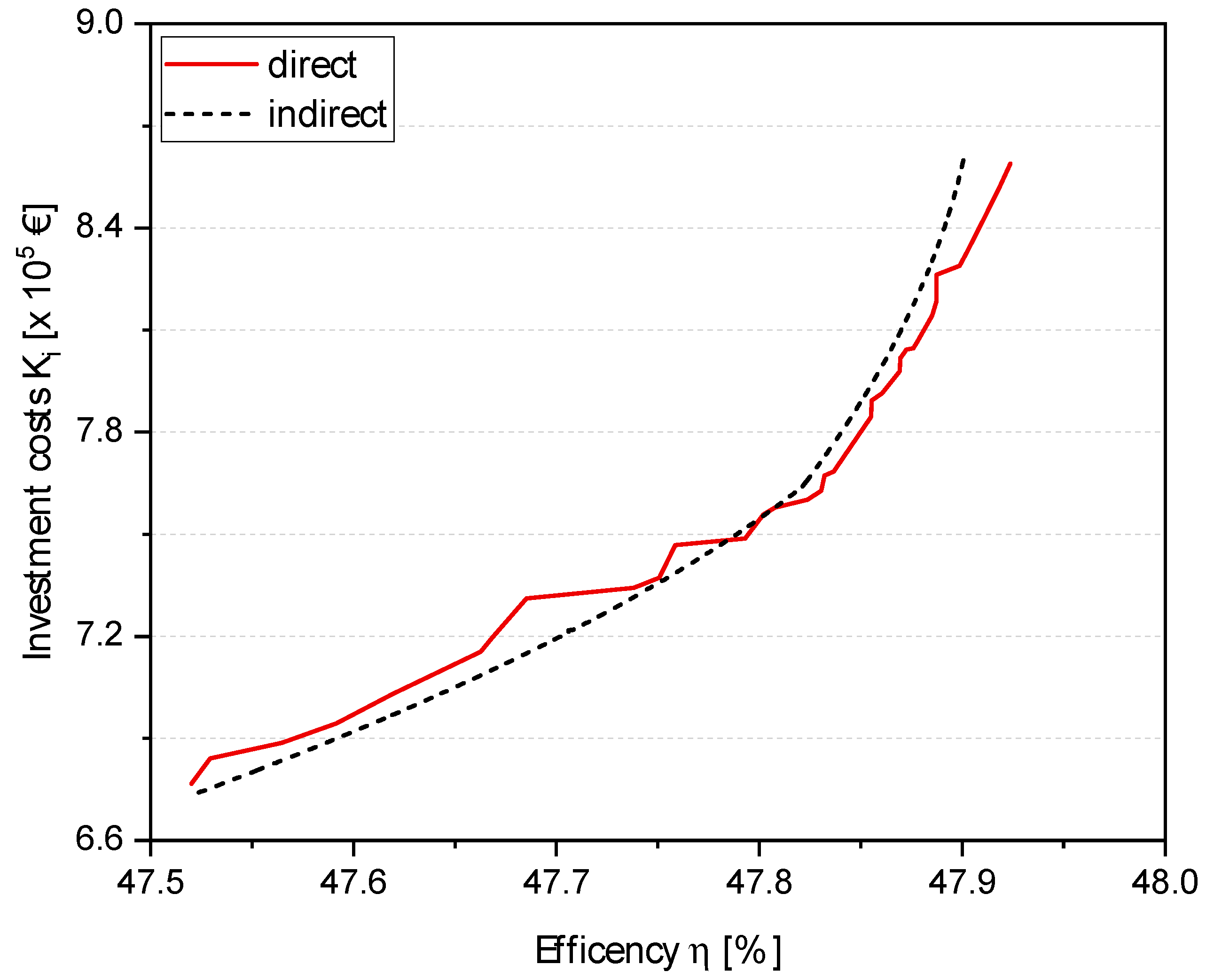
When using approximations, it must be taken into account that the results are affected by an error seen in Figure 8, which compares the Pareto front of the two methods. Whereas the indirect Pareto front generates a very smooth graph, the direct method shows a much more complex behavior. The use of the approximation simplifies the system response, which in this example leads to areas where the investment costs are underestimated or overestimated. Because of these discrepancies, the indirect method should be used primarily as a first optimization step in order to reduce the overall computing time and to locate/constrain the relevant solution space [5].

With increasing model runtime, shortening methods become more important. If no pre-optimization is desired, parallelization methods can be used alternatively. Since the simulations of each evaluation loop are executed parallelly instead of sequentially, runtime reductions can be achieved without affecting the result. In the present work, the runtime of the direct method could be reduced by up to 75% using parallelization. A further reduction can be realized by using a computing cluster that grants access to more cores.

6.3. Comparison of the DLR Optimization Library and optiSLang

In the following section, a comparison of the optiSLang workflow and the DLR Optimization Library is presented. Since the DLR Optimization Library uses weighting to transform multi-objective problems into single-objective problems, no comparison to the previous results could be made. Instead, a single-objective optimization using the overall efficiency as the optimization goal is carried out. An evolutionary algorithm with standard specifications is used for the calculation, and parallelization methods are considered.

All setups manage to improve the overall system efficiency (see

Table 3. Overall runtime and maximum efficiency of the investigated setups for the single-objective optimization of the HP preheater.

Method	${\mathsf{\eta }}_{\mathit{o}\mathit{p}\mathit{t}}$$(∆\mathsf{\eta }$) [%]	${\mathsf{\eta }}_{\mathit{D}\mathit{L}\mathit{R},\mathit{d}\mathit{i}\mathit{r}\mathit{e}\mathit{c}\mathit{t}}-{\mathsf{\eta }}_{\mathit{o}\mathit{p}\mathit{t}}$ [%]	$\mathit{t}$ [h]	$\frac{\mathit{t}}{{\mathit{t}}_{\mathit{D}\mathit{L}\mathit{R},\mathit{d}\mathit{i}\mathit{r}\mathit{e}\mathit{c}\mathit{t}}}$ [-]
DLR Optimization Library direct	51.688 (+0.105)	0	11.4	1
DLR Optimization Library direct and parallel	51.688 (+0.105)	0	5.3	0.46
optiSLang direct	51.689 (+0.106)	0.001	8.2	0.72
optiSLang direct and parallel	51.689 (+0.106)	0.001	2.1	0.18
optiSLang indirect	51.686 (+0.103)	−0.002	7.2	0.63

). The optimized efficiency ${\mathsf{\eta }}_{opt}$ as well as the difference from the initial value $∆\mathsf{\eta }$ are shown in the second column of the table and only differ slightly. For further comparisons of the setups, the direct DLR setup is defined as a reference. With regard to the optimized efficiency, only minimal changes occur. On the other hand, large differences in the runtime were found. The direct optimization of the DLR Optimization Library is the most time-consuming setup. However, by using parallelization, the runtime can be more than halved. The direct optiSLang setup reduces the runtime by almost 40%. By using additional parallelization, the runtime can be further reduced by a factor of 5.4 without influencing the results. The indirect optiSLang setup is faster than the direct DLR and direct optiSLang setup but slightly influences the optimized results negatively. A benefit of this setup is the generated surrogate model, which can be reused for further optimization runs.

7. Conclusions

Since the programming language Modelica does not allow for the definition of optimization problems, it is necessary to link up with external optimization environments or optimization languages. The simulation environment Dymola offers the integrated DLR Optimization Library, which contains ready-made methods for static and transient optimization. These optimization methods are easy to use but only customizable to a limited extent. Therefore, it is barely possible to adapt the algorithm individually for different optimization tasks. Since the optimization is achieved directly, large simulation models cause long optimization times. For a runtime reduction, parallelization can be used. To ensure a better optimization performance with higher flexibility, tools such as Ansys optiSLang can be used. An implementation of an appropriate workflow for coupling Modelica/Dymola and optiSLang is presented in this paper. It has been shown that the optimization via optiSLang can be more time-efficient compared to the Dymola standard DLR Optimization Library. When using parallelization and indirect optimization with surrogate models, the runtime of the examined test case has been reduced by a factor of 5.4. This improvement is necessary to deal with large-scale optimization problems in a suitable time. By using the sensitivity analysis, it is possible to obtain additional information about the system behavior. The determined surrogate model (meta model) can also be used for an indirect optimization, which is especially advantageous for a repeated optimization of the same model. Due to the deviations from the model behavior, indirect methods should only be used for pre-optimizations.

The comparison with the DLR Optimization Library shows that the developed workflow makes it possible to solve static optimization problems very efficiently. Further investigations should focus on optimization problems with a higher complexity to identify the limits of the presented workflow. In addition, the first investigations showed that dynamic optimization problems may be realized by adjusting the workflow. For this, the input signals/vectors need to be discretized into a finite number of static points, which can be used later like the tuners of the static optimization.

References

- Subramanian, A.; Gundersen, T.; Adams, T. Modeling and Simulation of Energy Systems: A Review. Processes 2018, 6, 238. [Google Scholar] [CrossRef]
- Akesson, J. Optimica—An Extension of Modelica Supporting Dynamic Optimization. The Modelica Association. 2008. Available online: https://www.researchgate.net/publication/253089188_Optimica-An_Extension_of_Modelica_Supporting_Dynamic_Optimization (accessed on 10 April 2023).
- Association, M. Modelica—A Unified Object-Oriented Language for Physical Systems Modeling Version 3.2 Revision 2. 2013. Available online: https://www.modelica.org/ (accessed on 10 April 2023).
- Dassault Systèmes; Dymola Dynamic Modeling Laboratory. 2022. Available online: https://www.3ds.com/ (accessed on 4 July 2022).
- Ansys optiSLang, Methods for Multi-Disciplinary Optimization and Robustness Analysis. Software Documentation, Version optiSLang 2022 R1. Available online: https://www.ansys.com/de-de/products/connect/ansys-optislang (accessed on 10 April 2023).
- Pfeiffer, A. Documentation, Optimization Library for Dymola: Version 2.2.2—Tutorial; Dassault Systèmes: Lund, Sweeden, 2016. [Google Scholar]
- Siebertz, K.; van Bebber, D.; Hochkirchen, T. Statistische Versuchsplanung: Design of Experiments (DoE); Springer: Berlin/Heidelberg, Germany, 2010. [Google Scholar]
- Göllmann, L.; Hübl, R.; Pulham, S.; Ritter, S.; Schon, H.; Schüffler, K.; Voß, U.; Vossen, G. Mathematik für Ingenieure: Verstehen Rechnen Anwenden: Band 2: Analysis in Mehreren Variablen, Differenzialgleichungen, Optimierung; Springer: Berlin/Heidelberg, Germany, 2017. [Google Scholar]
- Wünsch, A. Effizienter Einsatz von Optimierungsmethoden in der Produktentwicklung Durch Dynamische Parallelisierung. Ph.D. Thesis, Fakultät für Maschinenbau, Otto-von-Guericke-Universität Magdeburg, Magdeburg, Germany, 2016. [Google Scholar]
- Vogelsang, A.M. Mehrzieloptimierung von solarthermischen Parabolrinnenkraftwerken unter Berücksichtigung variabler Vergütungsschemata mit Hilfe technischer Auslegungsparameter. Ph.D. Thesis, Universität Flensburg, Flensburg, Germany, 2014. [Google Scholar]
- Graichen, K. Methoden der Optimierung und Optimalen Steuerung (WS 2017/2018). Ph.D. Thesis, Skriptum, Institut für Mess–; Regel– und Mikrotechnik, Universität Ulm, Institut für Mess–, Regel– und Mikrotechnik, Universität Ulm, Ulm, Germany, 2017. [Google Scholar]
- Vajna, S.; Bley, H.; Hehenberger, P.; Weber, C.; Zeman, K. CAx für Ingenieure: Eine praxisbezogene Einführung, 2nd ed.; Springer: Berlin/Heidelberg, Germany, 2009; Available online: http://site.ebrary.com/lib/alltitles/docDetail.action?docID=10274774 (accessed on 10 April 2023).
- Kallrath, J. Gemischt-Ganzzahlige Optimierung: Modellierung in der Praxis: Mit Fallstudien aus Chemie, Energiewirtschaft, Papierindustrie, Metallgewerbe, Produktion und Logistik, 2nd ed.; Springer: Berlin/Heidelberg, Germany, 2013. [Google Scholar]
- Schumacher, A. Optimierung Mechanischer Strukturen: Grundlagen und Industrielle Anwendungen, 2nd ed.; Springer: Berlin/Heidelberg, Germany, 2013. [Google Scholar]
- Pieper, M. Mathematische Optimierung: Eine Einführung in die Kontinuierliche Optimierung mit Beispielen (Essentials); Springer Fachmedien Wiesbaden: Wiesaden, Germany, 2017. [Google Scholar]
- Mu, B.; Li, Y.; House, J.M.; Salsbury, T.I. Real-Time Optimization of a Chilled Water Plant with Parallel Chillers Based on Extremum Seeking Control. Appl. Energy 2017, 208, 766–781. [Google Scholar] [CrossRef]
- Liu, F.; Deng, J.; Pan, W. Model-based Dynamic Optimal Control of an Ejector Expansion CO2 Heat Pump Coupled with Thermal Storages. Energy Procedia 2018, 152, 156–161. [Google Scholar] [CrossRef]
- Senthil, S.; Senthilmurugan, S. Reverse Osmosis–Pressure Retarded Osmosis hybrid system: Modelling, simulation and optimization. Desalination 2016, 389, 78–97. [Google Scholar] [CrossRef]
- Chen, J.; Garcia, H.E. Economic optimization of operations for hybrid energy systems under variable markets. Appl. Energy 2016, 177, 11–24. [Google Scholar] [CrossRef]
- Hoffmann, C.; Puta, H. Dynamic optimization of energy supply systems with modelica models: Energy saving control in plants and buildings. IFAC Proc. Vol. 2006, 39, 51–56. [Google Scholar] [CrossRef]
- Gräber, M. A tool chain for the efficient solution of optimal control point. Linköping Univ. Electron. Press 2017, 132, 249–254. [Google Scholar] [CrossRef]
- Karami, M.; Wang, L. Particle Swarm optimization for control operation of an all-variable speed water-cooled chiller plant. Appl. Therm. Eng. 2018, 130, 962–978. [Google Scholar] [CrossRef]
- Thieriot, H. Towards Design Optimization with OpenModelica Emphasizing Parameter Optimization with Genetic Algorithms. Available online: https://ep.liu.se/ecp/063/084/ecp11063084.pdf (accessed on 10 April 2023).
- Delikaya, G. Supervisory Control of a Combined Heat and Power Plant by Economic Optimization. Master’s Thesis, Fraunhofer ISE, Freiburg, Germany, 2015. [Google Scholar]
- Huang, S.; Zuo, W.; Sohn, M.D. Improved cooling tower control of legacy chiller plants by optimizing the condenser water set point. Build. Environ. 2017, 111, 33–46. [Google Scholar] [CrossRef]
- Granderson, J.; Lin, G.; Blum, D.; Page, J.; Spears, M.; Piette, M.A. Integrating diagnostics and model-based optimization. Energy Build. 2019, 182, 187–195. [Google Scholar] [CrossRef]
- Ali, M.; Vukovic, V.; Sahir, M.H.; Fontanella, G. Energy analysis of chilled water system configurations using simulation-based optimization. Energy Build. 2013, 59, 111–122. [Google Scholar] [CrossRef]
- Pfeiffer, A. Numerische Sensitivitätsanalyse Unstetiger Multidisziplinärer Modelle mit Anwendungen in der Gradientenbasierten Optimierung. Ph. D. Thesis, Martin-Luther Universität Halle-Wittenberg, Halle, Germany, 2008. [Google Scholar]
- Riedel, J. Gewichtsoptimierung eines Kreuzfahrtschiffes unter Spannungsrestriktionen; Institutskolloquium: Dynardo, Germany, 2000; Available online: https://www.dynardo.de (accessed on 25 January 2020).
- TLK-Thermo GmbH and XRG-Simulation GmbH, Clara Lib—Version 1.4.0. 2019. Available online: https://www.claralib.com/ (accessed on 20 March 2020).
- Branke, J.; Deb, K.; Miettinen, K.; Słowiński, R. Optimization, M.5252; Springer: Berlin/Heidelberg, Germany, 2008. [Google Scholar]
- Lehner. Betriebstechnik—BET -Wirtschaftlichkeitsrechnungen und Betriebliches Rechnungswesen. Available online: https://docplayer.org/14249839-Betriebstechnik-bet-teil-2-wirtschaftlichkeitsrechnungen-und-betriebliches-rechnungswesen.html (accessed on 16 January 2023).
- Lühe, C. Modulare Kostenschätzung als Unterstützung der Anlagenplanung für die Angebots- und frühe Basic Engineering Phase. Ph. D. Thesis, Technischen Universität Berlin, Berlin/Heidelberg, Germany, 2013. [Google Scholar]
- Zitzler, E.; Laumanns, M.; Thiele, L. SPEA2: Improving the Strength Pareto Evolutionary Algorithm; ETH Zurich, Computer Engineering and Networks Laboratory: Zurich, Switzerland, 2001. [Google Scholar] [CrossRef]