Article

Application of Fuzzy Neural Networks in Combustion Process Diagnostics

1
Department of Electronics and Information Technology, Lublin University of Technology, Nadbystrzycka St. 38D, 20-618 Lublin, Poland
2
School of Digital Technology and Artificial Intelligence, D. Serikbayev East Kazakhstan State Technical University, Protozanov St. 69, 070004 Ust-Kamenogorsk, Kazakhstan
3
Departament of Automation and Control, Satbayev University, Satpaev St. 22a, 050013 Almaty, Kazakhstan
4
Faculty of Information Technology, M.Kh. Dulaty Taraz Regional University, Tole Bi St. 40, 080000 Taraz, Kazakhstan
5
Faculty Artificial Intelligence and Big Data, Al-Farabi Kazakh National University, Al-Farabi Ave. 71, 050040 Almaty, Kazakhstan
*
Author to whom correspondence should be addressed.
Energies 2024, 17(1), 212; https://doi.org/10.3390/en17010212
Submission received: 27 November 2023 / Revised: 15 December 2023 / Accepted: 28 December 2023 / Published: 30 December 2023
(This article belongs to the Section I2: Energy and Combustion Science)

Abstract

:
Coal remains one of the key raw materials used in the energy industry to generate electricity and heat. As a result, diagnostics of the combustion process is still an important topic of scientific research. Correct implementation of the process allows the emission of pollutants into the atmosphere to be kept at a compliant level. Therefore, it is important to conduct the process in a manner that will not exceed these standards. A preliminary analysis of the measurement signals was carried out, and signal predictions of flame intensity changes were determined using the autoregressive moving average (ARMA) model. Different fuzzy neural network architectures have been investigated. Binary and multi-class classifications of flame states were conducted. The best results were obtained from the ANFIS_grid partition model, producing an accuracy of 95.46% for binary classification and 79.08% for multi-class classification. The accuracy of the recognition of flame states and the high convergence of the determined predictions with measurement signals validate the application of the proposed approach in diagnosing or controlling the combustion process of pulverized coal and its mixtures with biomass. Expert decisions determine the range of acceptable states.

1. Introduction

In its basic assumptions, the European Union’s energy policy focuses on the continued development of renewable energy sources while moving away from conventional energy. In Poland, according to the adopted energy strategy, the use of coal in the power sector will decrease significantly [1]. However, despite the planned changes, lignite, hard coal, and coking coal are still among the list of strategic raw materials for the Polish economy. In addition, coking coal is considered a critical resource for the economy of Poland and the European Union [2]. Another aspect is the lack of energy independence of EU member states, which is particularly noticeable in the context of political crises. Until the EU’s energy strategies are fully implemented, coal will continue to be one of the pillars of the energy sector. This makes the need for further development of methods for the analysis and processing of coal as a raw material still actual and necessary.
In the power industry, pulverized coal combustion is a complex process that, in terms of control, monitoring, and diagnostics, requires specialized measurement systems. These technologies are constantly being improved [3,4,5,6,7,8,9]. The combustion process should proceed efficiently, meaning the stability of combustion conditions is ensured and the emissions of the resulting pollutants are within the ranges of applicable standards. Direct combustion of pulverized coal is carried out using primary and secondary air. The primary air stream transports pulverized coal to the burner [10,11], and the supplied secondary air stream allows the combustion process to occur. Direct combustion is the primary technology for processing coal fuel, and it is constantly being studied to reduce the resulting pollutants [12,13,14,15,16,17]. The formation of harmful combustion products is typically associated with the combustion of elemental carbon and hydrocarbons. Carbon dioxide CO2 is the product of the complete combustion process of the element carbon.
In contrast, carbon monoxide, soot, aromatic hydrocarbons, or aldehydes are produced by incomplete combustion. The chemical composition and presence of admixtures in the fuel also affect the occurrence of by-products in the combustion process. Among them are NOx, SOx, and ash [10,11]. Primary and secondary methods are commonly used to reduce emissions of harmful compounds from the pulverized coal combustion process. Primary methods are implemented directly in the combustion chamber and aim to prevent or reduce unwanted combustion products, such as low-emission combustion [18,19]. Secondary methods outside the combustion chamber are based on eliminating harmful combustion products using catalytic reduction [20,21] and absorption methods [10,11].
Using biomass as a fuel in the combustion process contributes to reducing emissions of pollutants—especially sulfur and nitrogen oxides. The process of co-firing pulverized coal and biomass can be carried out using co-firing technologies, i.e., direct, indirect, and parallel. In the direct co-firing method, pulverized coal and biomass form a fuel mixture that is supplied and simultaneously burned in the combustion chamber. Due to the complexity of the co-firing process, several monitoring and diagnostic methods are used, particularly for process stability and efficiency [22,23,24,25,26,27].
The efficiency of the combustion process can be affected by many factors, such as the speed and amount of fuel delivered to the combustion chamber or its chemical composition. Therefore, selecting an appropriate diagnostic method for the process is essential. The primary goal for combustion process diagnostics is the early detection of conditions indicative of process malfunction. These measures are designed to maintain adequate process efficiency and stability, prevent economic losses from potential failures, and support environmental protection. In the diagnostics of the combustion process, it is crucial to detect and recognize the transition from a stable to an unstable state, which can occur due to a change in process parameters or the appearance of disturbances. The problem of recognizing flame states in an individual burner is still being developed [28,29,30,31,32,33,34,35,36,37].
Measurement data from the combustion process can be acquired using optical methods whereby information is extracted from the flame in a non-invasive way. Among a number of monitoring systems are those based on thermal imaging cameras [38,39] and fiber-optic probes [40]. Monitoring systems that rely on optical technologies acquire and process information from the flame in real time. Their undoubted advantage is the ability to carry out measurements in dusty and high-temperature conditions. The fiber-optic probe is placed in the combustion chamber directly next to the burner so that, when monitoring fuel combustion, it can record measurement data from the flame for the various zones monitored by the probe. This technology ensures the acquisition of effective diagnostic parameters contained in the intensity of the flame. Measurement data are recorded in the form of a time series.
Despite the many advantages of combustion monitoring systems and the acquisition of detailed information from the flame, there is a need for further processing of measurement results. Measurement data processing is a significant research problem [41,42]. Therefore, many methods are used in the diagnosis, monitoring, and control of the combustion process, among which can be highlighted the Fourier transform [43], wavelet analysis [44], or recurrent neural networks [45,46,47,48,49,50]. Diagnostics of the combustion process can also use classification [51,52,53,54] and prediction [55,56].
Fuzzy neural networks are a combination of neural network structures and fuzzy logic. They are characterized by solid integration of expert knowledge into the system. These structures are based on fuzzy inference, similar to human inference, and thus considered more understandable [57]. Fuzzy neural network models are considered flexible and interpretable, and their features include the possibility of validation and modification [58,59]. Due to numerous advantages, fuzzy neural networks are suitable for solving diagnostic problems and monitoring the combustion process.
In addition, fuzzy neural networks can solve various process diagnostic problems such as classification [60] and prediction [61]. In the area of combustion process analysis, fuzzy models have found application in carrying out diagnostics on the operation of a pulverized coal burner [62], modeling NOx emissions from a turbulent flame [63], and others.
Therefore, there is still a need to develop diagnostic methods for the combustion process to maintain stable conditions for the process and early identification of possible disturbances. Methods for classifying the states of a flame recognized by changes in its luminous intensity are a critical aspect of monitoring the combustion process. This paper proposes signal predictions of flame intensity and the use of fuzzy neural networks to recognize flame states.

2. Materials and Methods

2.1. Measurement System

Measurements of parameters of combustion processes can be carried out both in industrial facilities and specialized laboratory stations. Figure 1a shows the test stand, which comprises a cylindrical combustion chamber with a pulverized coal burner mounted in it. This system can burn fuels such as pulverized coal and a mixture of coal and biomass. These fuels are supplied to the burner using a dust tube. A system of measurement sensors is built into the bench to record fuel expenditures, average chamber temperatures, and primary and secondary air flows in real time through a data acquisition system.
The flame diagnostics process requires specialized measurement systems that will non-invasively acquire information about the combustion process. The flame monitoring system developed at the Department of Electronics of Lublin University of Technology [40,64] was used to acquire measurement data from the flame. A schematic of the system for acquiring data from the flame is shown in Figure 1b.
The most critical components in a flame monitoring system are the measuring probe, photodetectors, and the signal processing block. In the construction of the measuring probe, it is necessary to distinguish the probe head with a bundle of optical fibers, which is placed inside the combustion chamber near the burner. The design of the optical probe allows it to operate in high temperatures, high vibration, and dusty conditions. The measuring probe is placed in the combustion chamber through an inspection hole near the burner. With the fiber-optic head, it is possible to acquire data from the flame in several zones along its axis. The optoelectronic block is built with four twin signal paths (marked in Figure 1b with numbers 1–4), which allow monitoring of different flame zones marked by shades of gray also in Figure 1b. Then, the measurement data are transferred to the optoelectronic block and converted into an electronic signal, which is further processed.
The research was conducted using a fiber-optic flame monitoring system. It was implemented for its different flame zones utilizing a fiber-optic probe placed in the combustion chamber in an inspection hole. The design of the probe used for the research allows measurements to be taken in zones at different distances from the flame front. The flame intensity is a measure of the amplitude of the signal recorded by the detector, which is proportional to its temperature. The range of radiation used in the measurements is from the visible to near-infrared region and is conditioned by the spectral characteristics of the detector used. Vortex burners are used in the combustion process of pulverized coal and its mixture with biomass. The intensity of fuel–air mixing depends on the amount of primary air (the air used to transport the fuel) and secondary air. The vortices that appear cause the flame to pulsate (the intensity of its glow changes). Measuring these changes, i.e., changes in radiation intensity, can be used to both assess the state of the process and control it. These changes are caused by the turbulent movement of the flame during the combustion process. They are characteristic of separated zones (Figure 1b) in the combustion process.

2.2. Analysis of Measurement Data

Studies of changes in flame intensity were conducted for two types of fuel: 100% pulverized coal and a mixture of 80% coal and 20% biomass. The measurement results presented in the paper were performed on a combustion research stand under the following conditions: thermal power—400 kW and excess air ratio λ = 0.85. During the research, the fuel composition did not change.
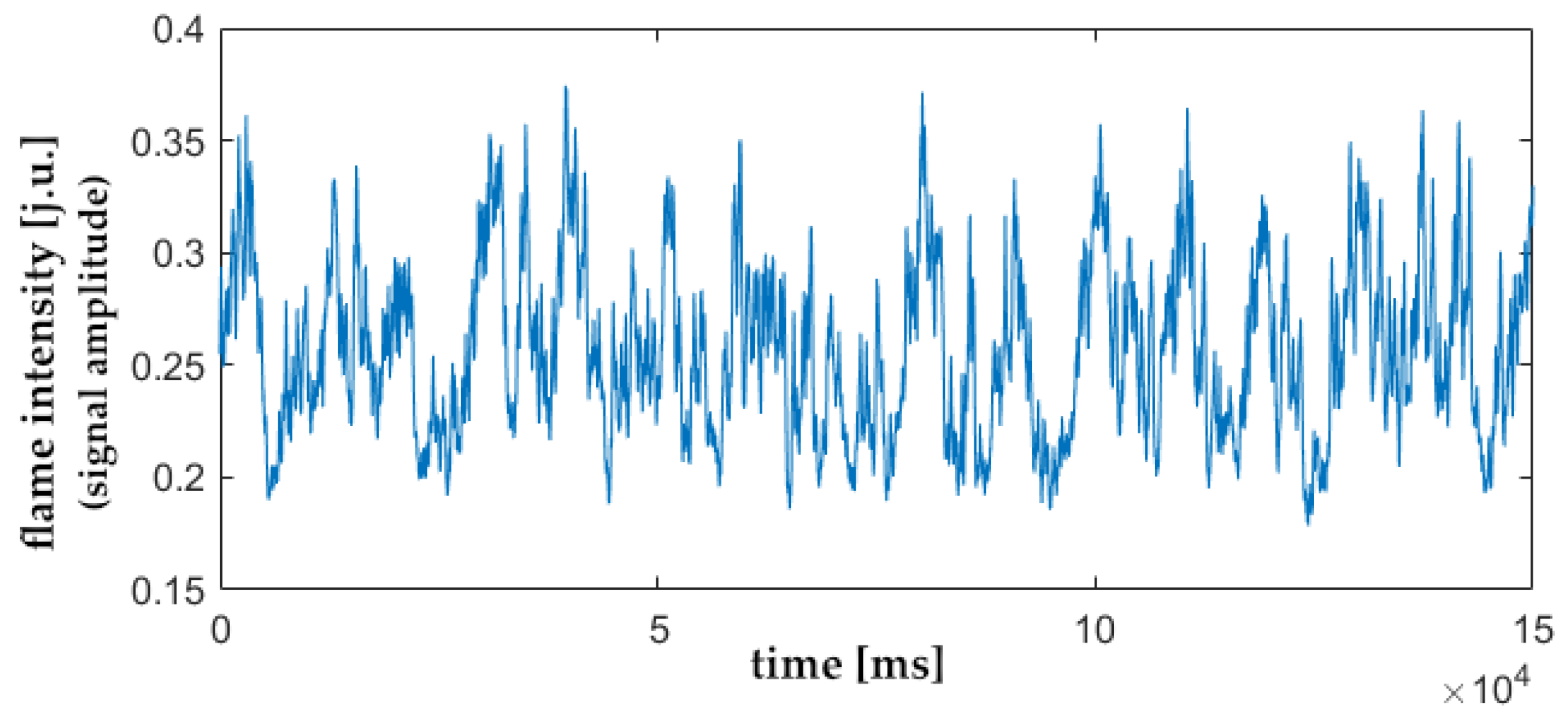
Each dataset contains more than 2 million samples, which were taken at 1 kHz and come from four channels of the fiber-optic probe. The data were recorded as a time series. Figure 2 shows an example of a time series for changes in flame intensity for pulverized coal.
When adjusting the power generated by a power boiler, the need to change its operating point arises, leading to short-term trends in the monitored flame. The speed and magnitude of these changes can be observed as linear or non-linear trends. These can lead to an increase in undesirable combustion products, such as NOx, SOx, or CO, or to flameout, which can occur when adjusting for minimum load (less than 50% power). Based on expert consultations, ranges have been determined beyond undesirable effects (an increase in pollution or the possibility of flameout). Time series variability forecasting can be used in diagnostics or controlling pulverized coal combustion or its mixture with biomass. For this, it is necessary to determine their mathematical models, which for linear series belong to the ARMA class, and for non-linear series—ARIMA.

2.3. Flame Time Series Predictions Using the ARMA Model

The autoregressive moving average (ARMA) (p,q) model is described by components that determine [65,66]:
-
p—the number of autoregression parameters,
-
q—the number of parameters of the moving average.
It is expressed by the following relation [65,66,67]:
x t ~ = φ 1 x ~ t 1 + φ 2 x ~ t 2 + + φ p x ~ t p + a t θ 1 a t 1 θ 2 a t 2 θ q a t q
where   x ~ t —the deviation from the average value,   φ i —the weighting factors of the autoregressive component,   θ i —the weighting factors of the moving average component, and a —a sequence of random variables.
Differentiation of the analyzed flame time series was made for cases where trends appeared before the determination of forecasts. Therefore, it was possible to determine the ARMA (1.1) model. The next step in the implementation of the research was to recognize the occurrence of trends in flame intensity signals using neural networks.

2.4. Classification of Flame States

Fuzzy neural networks were used to classify flame states. The classification was carried out for two variants of recognition of 2 and 6 flame features. The first variant of flame state classification recognized 2 features as a “stable” state (0) and an “unstable” state (1). The other variant recognized 6 states:
  • 0—stable,
  • 1—flame with a rising exponential trend,
  • 2—flame with an exponential downward trend,
  • 3—flame with an increasing linear trend,
  • 4—flame with a descending linear trend,
  • 5—state of fading flame.
A dataset with 402,000 observations was created for analysis. The data was divided into a training set of 282,000 samples and a test set of 120,000 observations. The measurement data were divided into a ratio of 70.15% training set and 29.85% test set. The following metrics were adopted to evaluate network parameters:
  • True Positive Rate (TPR)—a measure of the probability of correct classification for the class “stable” if the case belongs to this class. It is expressed by the relation:
T P R = T P T P + F N ,
where True Positive (TP)—the number of stable cases classified as stable and False Negative (FN)—the number of stable cases classified as unstable.
  • True Negative Rate (TNR)—a measure of the probability of correct classification for the class “unstable” if the case belongs to this class. It is expressed as follows: True Negative (TN) is the number of unstable cases classified as unstable, and False Positive (FP) is the number of unstable cases classified as stable.
  • Accuracy (ACC)—a parameter that evaluates what the probability of correct classification of cases is that belong to both classes, e.g., stable and unstable. It is calculated from the equation:
A C C = T P + T N T P + T N + F P + F N .
  • Precision (PRE)—a parameter that evaluates what number of selected observations is accurate. It is calculated from the equation:
P R E = T P T P + F P .
  • F1 Score—a value based on precision and sensitivity parameters; it is calculated as follows:
F 1 = 2 · P R E · R E C P R E + R E C .
Adaptive Neuro-Fuzzy Inference System (ANFIS) is a type of artificial neural network based on the Takagi–Sugeno fuzzy inference system. The network structure can be distinguished into two parts: the premise part and the consequence part. In analyzing the architecture in detail, it consists of five layers. The first layer takes the input values and determines the membership functions belonging to them. The second layer is responsible for generating rules. Because of its task, this layer is called the “rules layer”. The role of the third layer is to normalize calculations. The fourth layer takes normalized values as input, which are returned with defuzzified values and are passed to the last layer to produce the final result [67].

3. Results and Discussion

3.1. Statistical Analysis of Flame Signals

To assess the sensitivity of flame signals from individual probe channels, fundamental statistical values, i.e., maximum, minimum, average, RMS, standard deviation, and coefficient of variation, were calculated for selected zones. To assess the sensitivity of flame signals from individual probe channels, fundamental statistical values, i.e., maximum, minimum, average, root mean square, standard deviation, and coefficient of variation, were calculated for selected zones. The example time series of flame signals for which statistical parameters were determined is plotted in Figure 3.
The results of the analysis of flame parameters for selected signals are included in Table 1. The values shown in the table are for sample measurement signals 1–3, which represent changes in flame intensity for 100% pulverized coal and were measured for four channels of the optical probe. Measurement data 4–6 represent flame intensity signals for a mixture of 80% pulverized coal with 20% biomass.
It was found that in most measurements, the coefficient of variation, which is a measure of the variation of features in the signal, would reach the highest values for data from the first flame zone [67,68,69,70]. The coefficient of variation for the signals was determined from the equation:
V = σ x ¯ ,
where   σ —standard deviation and x ¯ —arithmetic mean value.
A statistical analysis of the flame signals confirmed that the first channel of the optical probe is the most sensitive. This channel records measurements closest to the flame nucleus.

3.2. Correlation Coefficient

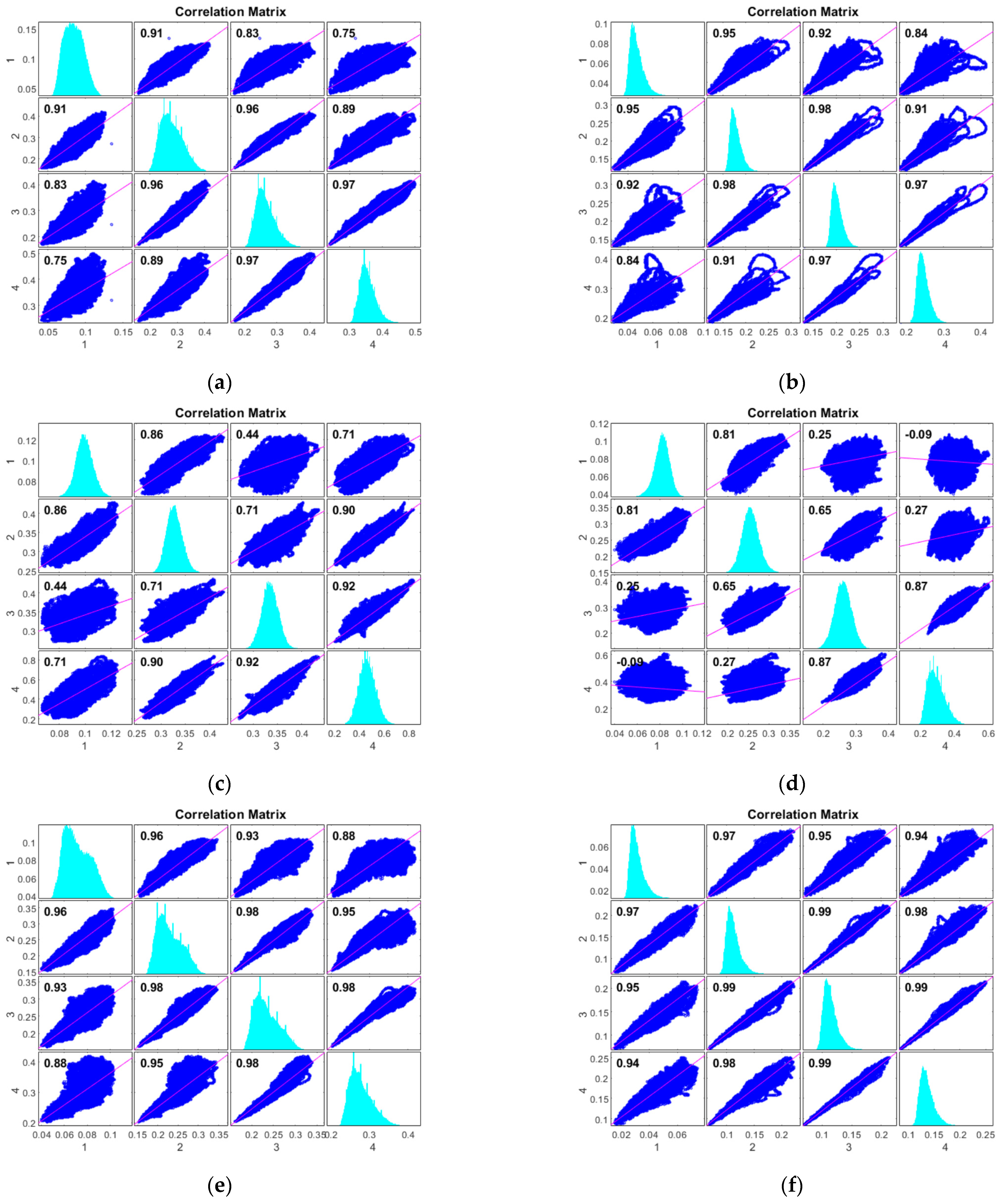
The correlation between each of the four channels was then examined using Pearson’s correlation coefficient [67,68,69,70]. Each subgraph, off the diagonal, includes a scatter plot of a pair of variables with a least squares reference line. The slope of this line is equal to the correlation coefficient displayed in the upper left corner. On the other hand, each diagonal subgraph contains the distribution of the variable represented as a histogram. Figure 4 shows time series correlation plots of flame intensity for fuels: 100% coal and a mixture of 80% pulverized coal and 20% biomass.
The optical probe captures information from the flame in different monitoring zones. From the analyses conducted for signals from different zones of the flame, it is clear that zone one is the most sensitive; for further studies, the measurement data will come only from the first zone.
Flame diagnostics in the combustion process is based on recognizing changes in the flame intensity. The occurrence of trends in the flame is crucial diagnostic information. Further analysis of the flame signals examined the flame time series for signal trends.

3.3. Determining Trends in Flame Signals

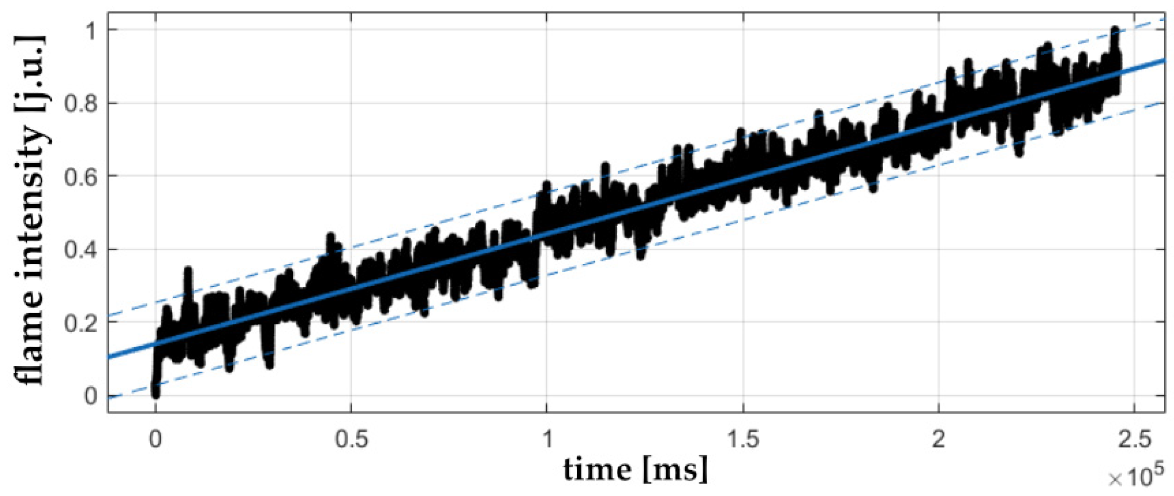
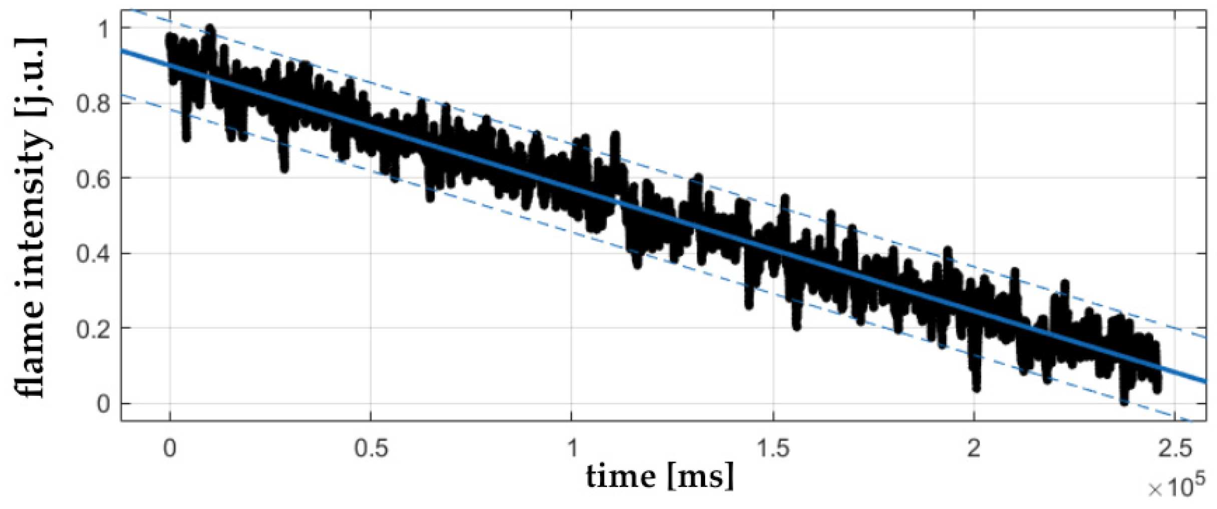
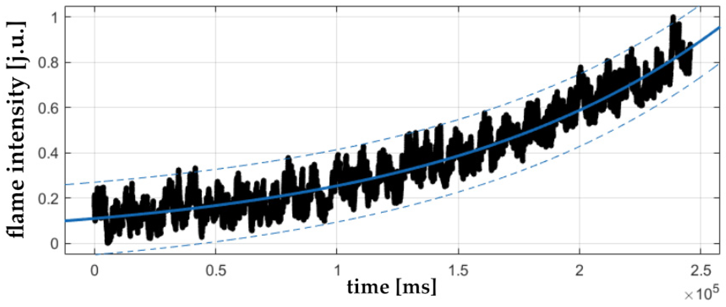
In the combustion process, determining emerging trends can contribute to the detection of disorders. Detection of any disorders in the ongoing combustion process requires particular observation because they can lead to deterioration of the safety balance of the combustion process. The following trends were determined in the analyzed signals using the function fitting method: linear and exponential with both decreasing and increasing nature. Figure 5, Figure 6, Figure 7 and Figure 8 show selected flame intensity measurement signals marked in black. Whereas the determined trends are represented by blue solid.
The coefficient of determination R2, which is a measure of the fit of the linear regression model to the measurement data, was calculated. The value of the coefficient of determination is in the 0–1 range [67]. The most extensive fit is obtained when the R2 value is close to 1. High matching was achieved for the flame measurement signals shown in Figure 6, Figure 7 and Figure 8. In the graphs, the blue dotted line indicates 95% confidence intervals. Table 2 shows the statistics by which it is possible to assess the quality of the fit of the determined trend to the signal.
The parameter Sum of Squares due to Error (SSE) is a random variability value that determines the sum of deviations of the total variability of all values from a simple regression, i.e., [67,68,69,70]:
S S E = i = 1 n y i y i ^ 2
where y i —the total variation of all values and y i ^ —the variation of values determined by the simple regression.
A value closer to zero indicates a match that is more useful for prediction. For the analyzed signals, the lowest value of the SSE parameter was obtained for the measurement signal of flame no. 25. The coefficient of determination R2 reached its lowest value in the case of the measurement signal for flame no. 1; in the other cases, the model’s fit to the measurement data was high. RMSE is the root of the root mean square error. Its value should be closer to 0. This indicates a match that is more useful for prediction. For all flame measurement signals analyzed, the number of coefficients in the model was two.
In summary, the analysis of the measurement data included a statistical evaluation of the flame signals, based on which the coefficient of variation for each channel of the optical fiber probe was determined. Then, also for the four channels, the correlation coefficient was examined. The first zone was found to have the highest sensitivity; therefore, further analysis of the measurement data can be limited. Based on the analysis, the measurement data were processed, and the ascendancy of trends in the time series of flame intensity signals was studied. These methods provide the basis for further analysis, prediction, and classification of flame states.

3.4. Flame Time Series Predictions Using the ARMA Model

ARMA models were determined to predict signals of changes in flame intensity. Measurement data with occurring trends have been differentiated. Detailed parameters were obtained for the ARMA (1.1) model, as shown in Table 3.
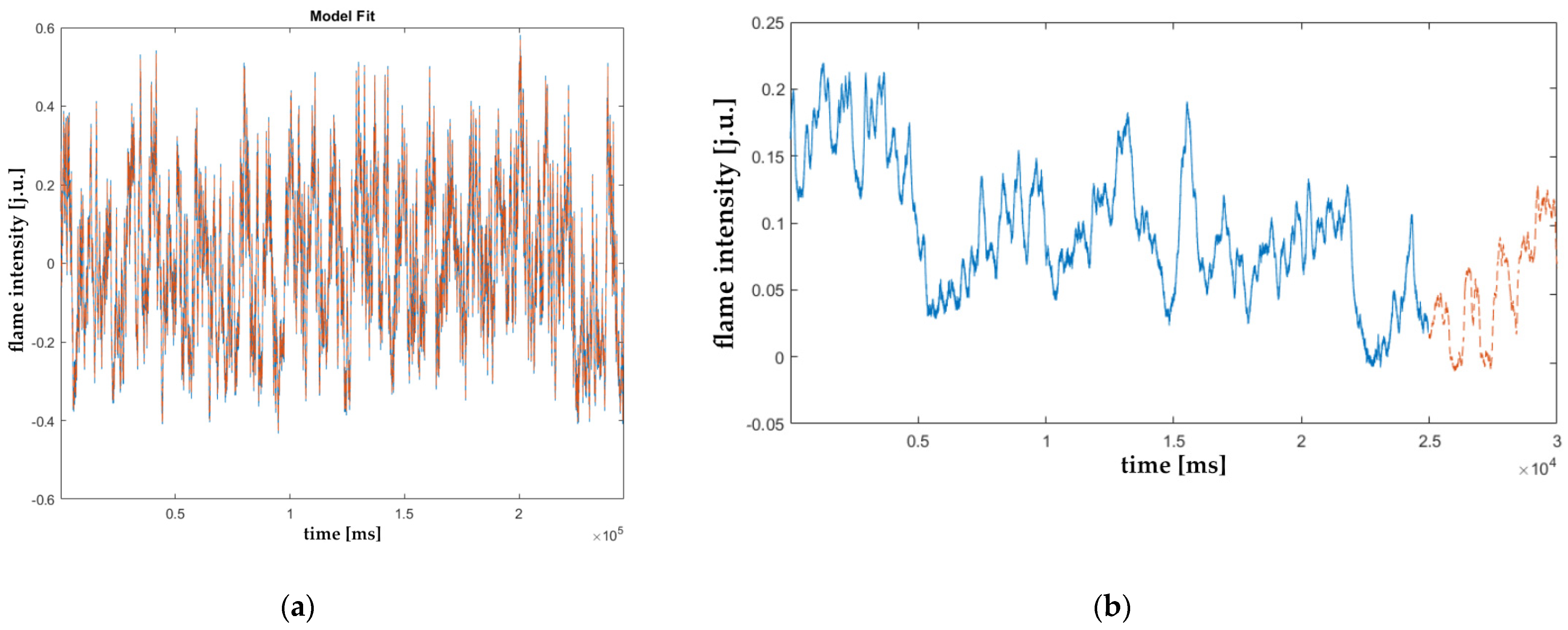
For the ARMA (1.1) model and the individual flame measurement signals, the values of the model parameters were determined, i.e., constant value, variance, and AR and MA components. In addition, the standard error and values of the t-statistic were calculated for each model parameter. Based on the ARMA model for the time series of changes in the intensity of the flame’s luminosity, one-step predictions were determined. The determined predictions are presented in the example of flame signal no. 1 for 100% pulverized coal in Figure 9. The blue color indicates the basic flame signal, and the red dotted line indicates the forecast.
In comparing the shape of the characteristics of the measurement data with the one-step forecast, shown in Figure 9a, it is essential to note a remarkable convergence. One-step predictions of flame intensity signals for 5000 steps are presented next. Figure 9b shows an excerpt of the flame signal along with the prediction. The measurement data are in blue in the 0–25,000 sample range, and the accompanying forecast in the 25,001–30,000 range is in red.
The ARMA model can be used to diagnose and control the combustion process. Due to their accuracy, one-step predictions are well suited for analyzing the changes occurring in the flame during the combustion process of pulverized coal or its mixture with biomass.

3.5. Classification of Flame States Using Fuzzy Neural Networks

To diagnose the combustion process, fuzzy neural network models were used to classify flame states. Binary and multi-class classifications were carried out. The first distinguishes whether the flame is stable or unstable. The other recognizes six different flame states: 0—stable, 1—flame with the exponential ascending trend, 2—flame with the exponential descending trend, 3—flame with the linear ascending trend, 4—flame with the linear descending trend, and 5—flame fading state.
Fuzzy neural networks using the ANFIS model were used to solve time series classification problems in the combustion process. The first element of the model, “genfisOptions” is the option for generating a fuzzy Sugeno type inference system. In the model, the fuzzy system is generated by grid partitioning—“GridPartition”, where the input membership functions are generated by evenly dividing the ranges of the input variables and forming a single-input Sugeno fuzzy system. The fuzzy rule base contains one rule for each combination of input membership functions. The following parameter was “NumMembershipFunctions”, defined as triangular membership functions. For the “InputMembershipFunctionType” parameter, the type of input membership function was specified as a Gaussian function. The next step in implementing the model was to present the rules. In addition, a set of options has been defined for the inference system object. The maximum number of “EpochNumber” training epochs has been defined as 200 epochs. The options for displaying ANFIS information “DisplayANFISInformation”, the parameter showing network learning error values, and the option for displaying final results “DisplayFinalResults” have been activated. ANFIS models were created for three variants of fuzzy system generation: grid partitioning (ANFIS_GP), subtractive clustering (ANFIS_SC), and fuzzy c-means clustering (ANFIS_FCM).
For the ANFIS_FCM model, cluster centers are calculated using fuzzy c-means clustering. In the case of binary classification, 33 iterations were required to determine the centers of the clusters, and the value of the objective function obj. fcn = 13.21 was obtained. For multi-class classification, 26 iterations were carried out, and the value of the objective function obj. fcn = 29.19 was obtained.
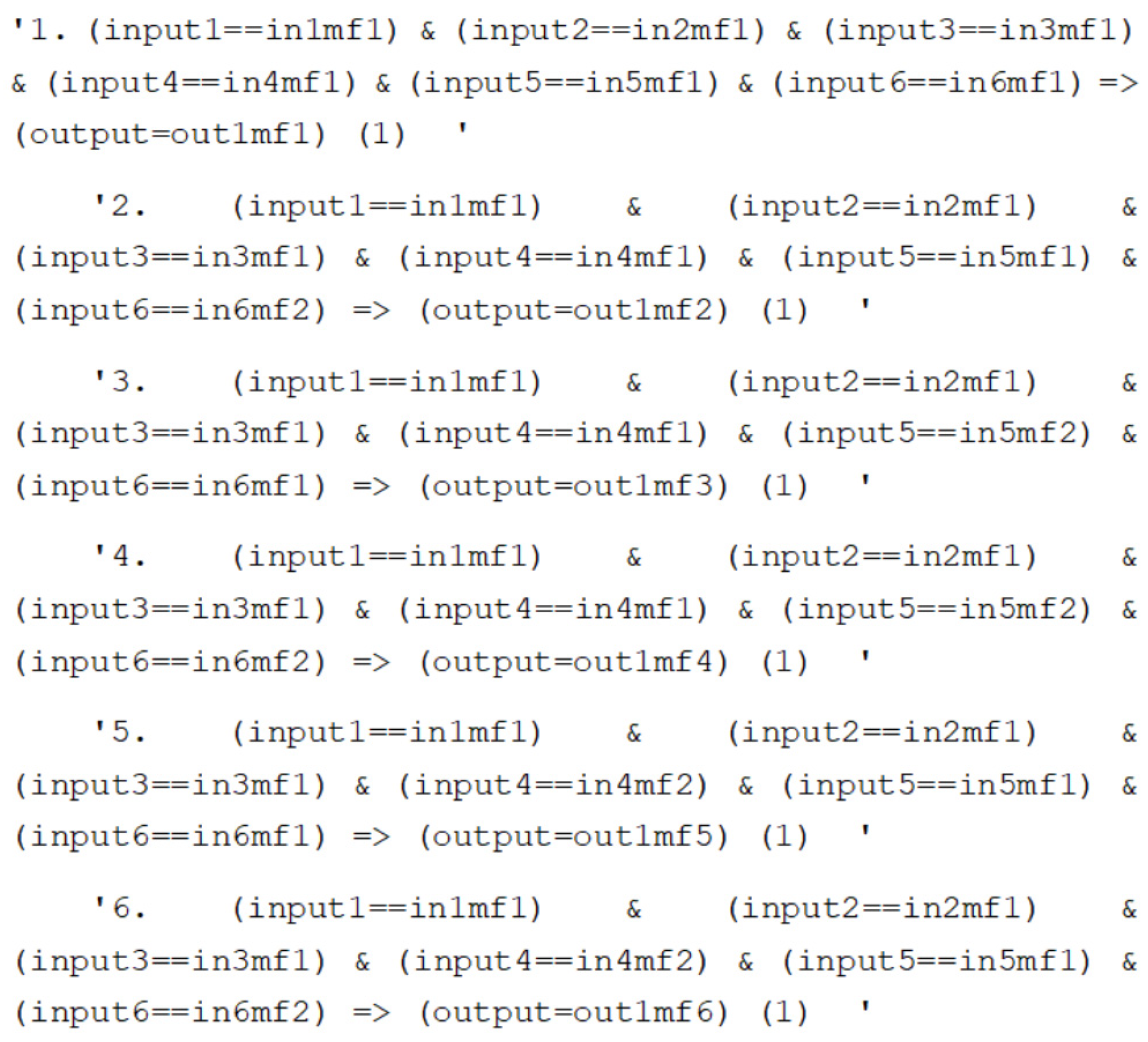
As a result of training the ANFIS networks, arrays of fuzzy rules have been obtained. An example of a fragment of the fuzzy rule table created for the ANFIS_GP model is shown in Figure 10.
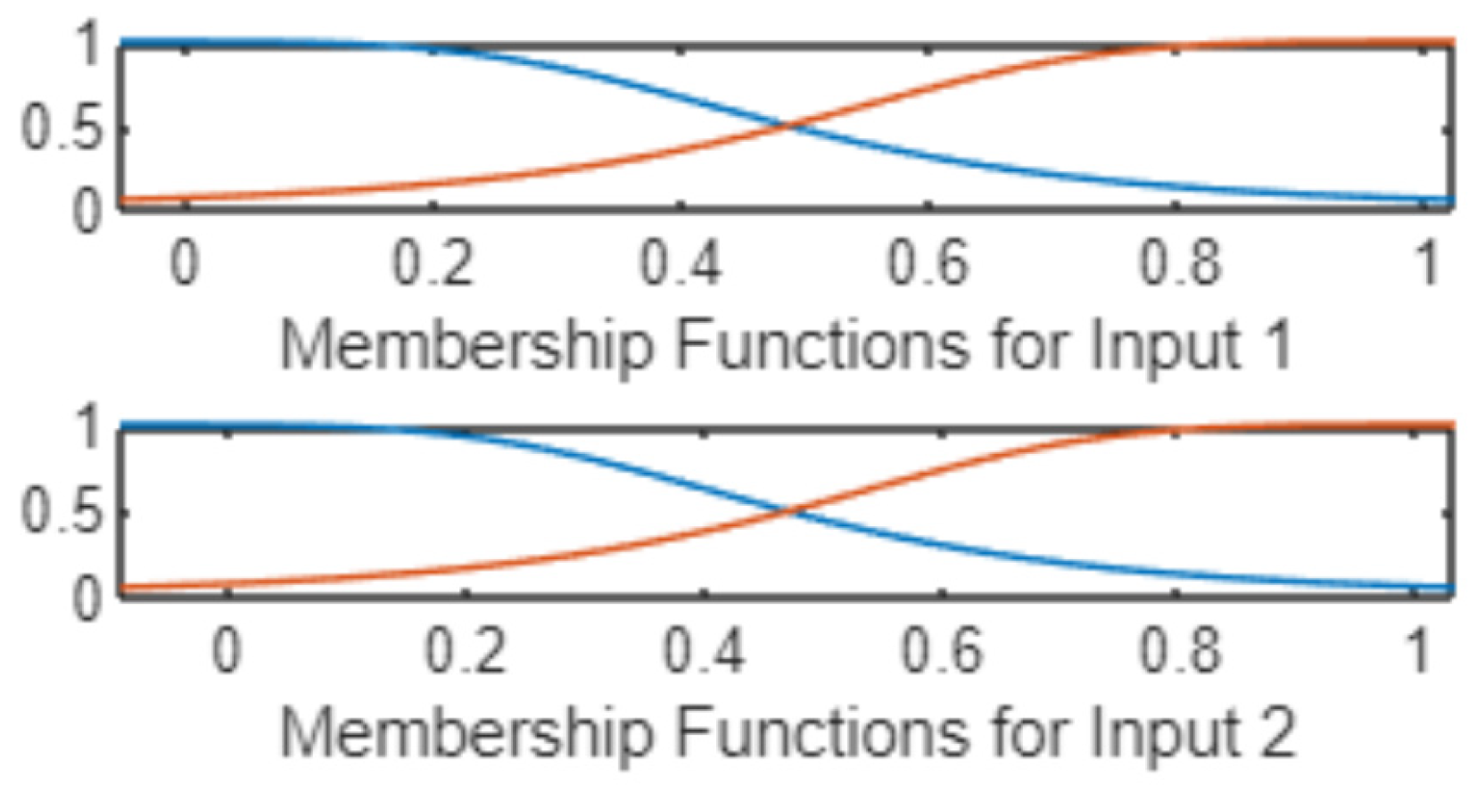
For each ANFIS model, membership functions are generated. Example functions for binary classification of flame states are shown in Figure 11.
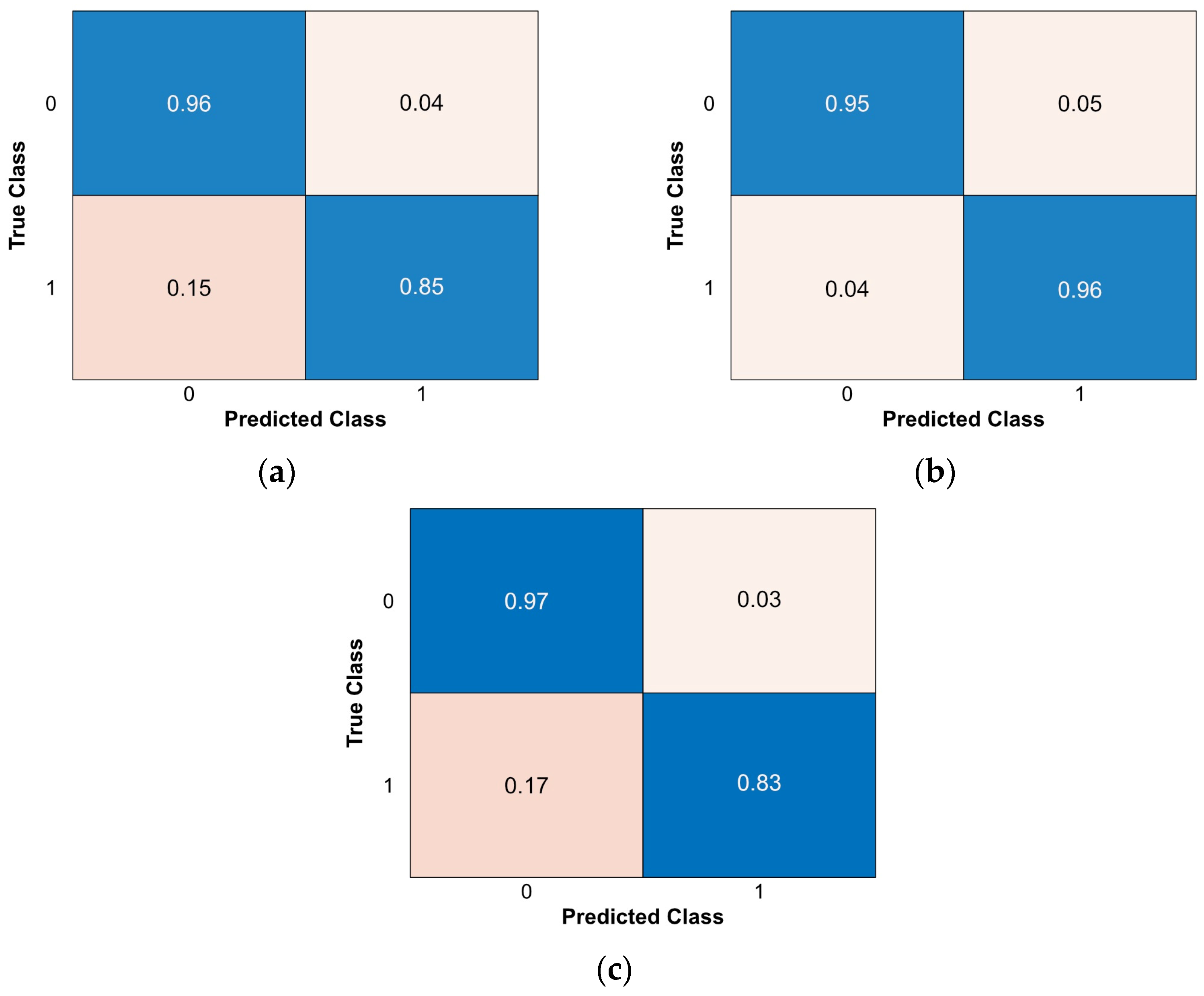
Figure 12 shows the normalized confusion matrices created for the three models that classify states. The stable state was labeled 0, and the unstable state was labeled 1. Parameters such as TP, FN, FP, and TN can be determined from these.
The various classification measures are presented in Table 4 and Figure 13 for bi-nary classification of flame state recognition. The highest accuracy was achieved for the ANFIS_GP model (ACC = 95.46%).
The various measures of classification are presented in Table 4.
In addition, a comparison of the various parameters of the models used was car-ried out, as shown in Figure 13.
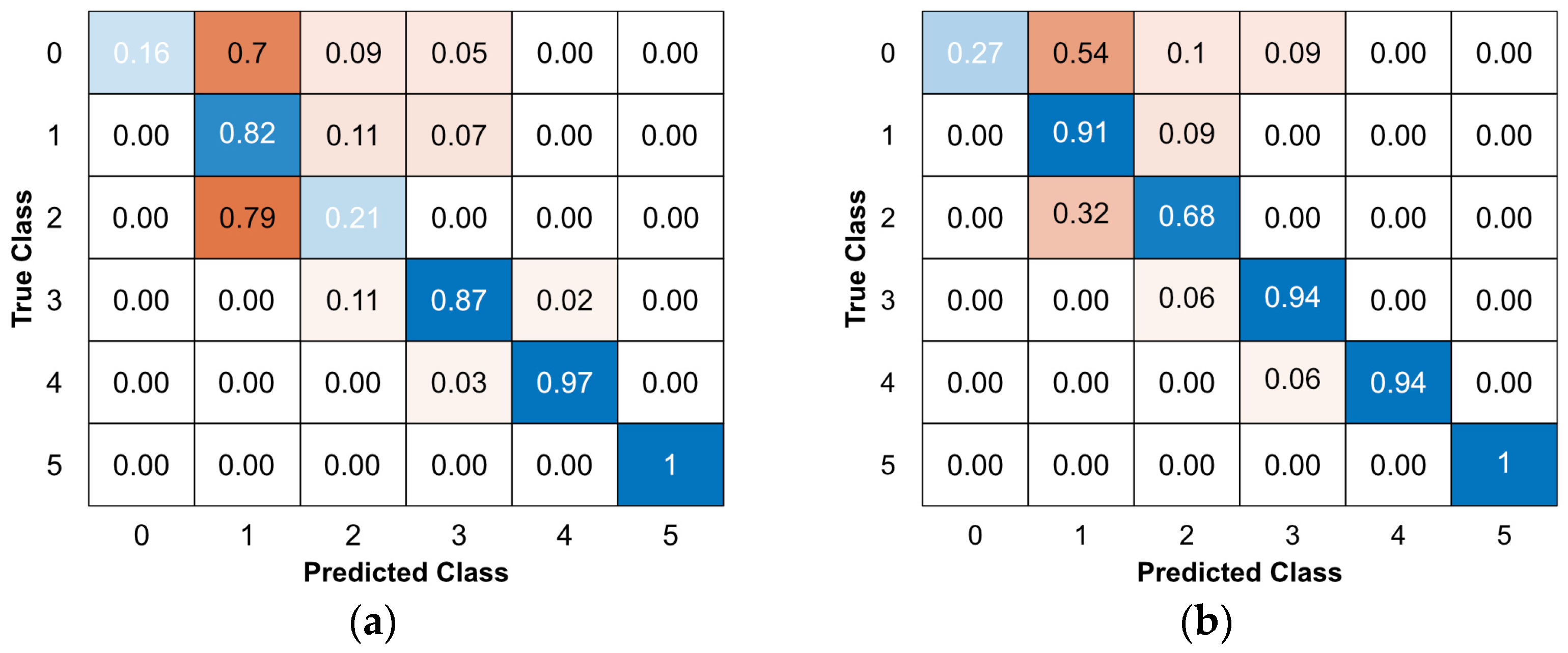
In addition, Figure 14 shows the normalized confusion matrices created for ANFIS models in configurations with grid partitioning (GP) and fuzzy c-means clustering (FCM) applied to classify 0–5 flame states. The ANFIS_GP model will achieve the most significant number of truly positive TP parameters.
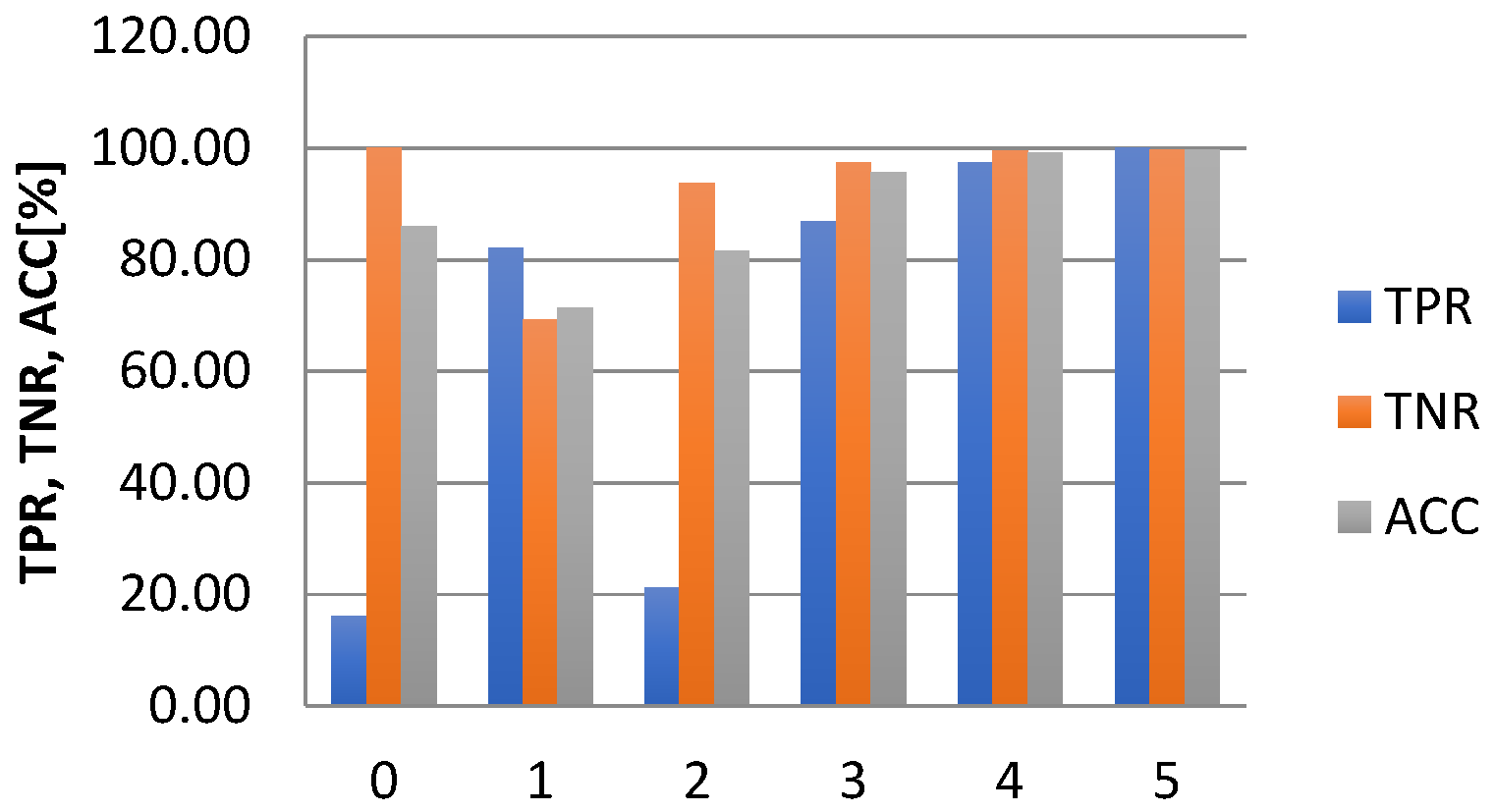
The parameters were determined for the models used for multi-class classification of flame state recognition, as shown in Table 5 and Figure 15.
For multi-class classification of flame states, the ANFIS_GP model achieved the highest accuracy (ACC = 79.08%). The highest sensitivity parameter values for both classification models were achieved with classes 1 and 3–5, while the lowest values were for classes 0 and 2. It should be noted that class 5 achieved the highest classification accuracy for both models. The comparison between fuzzy models classification accuracy is presented in Figure 16. In the figure, the results of binary classification are marked in orange and multi-class classification in blue.
In summary, fuzzy models have been used for binary and multi-class classifications of flame states. The ANFIS model with grid partitioning (GP) demonstrated the highest classification value, achieving ACC = 95.46% in the binary classification variant and ACC = 79.08% in the multi-class recognition variant.
The results show that with the created predictions using the ARMA model for the flame glow intensity measurement signals, it is possible to use the predictions practically for diagnostics and control of the combustion process.
In addition, using binary and multi-class classifications using fuzzy neural networks has proven highly effective in identifying flame states in the combustion of pulverized coal and its mixture with biomass. The proposed approach makes it possible to recognize flame states regardless of the type of fuel being burned. In addition, the proposed methods may be part of a system that diagnoses the combustion process in actual conditions taking place and supports the process operator.

4. Conclusions

Additional and actual information about the combustion process can be obtained based on flame changes. The selected methods and parameters will allow the development of an effective diagnostic system. The research results presented in this paper may constitute the basis for the development of and further research on such a diagnostic system.
The main component of this system is a fiber-optic measuring probe. Used for actual measurements, it meets the conditions for resistance to the effects of high temperatures. The acquisition of measurement data using measurement systems ensures the recording of substantial information about changes in the flame. In the monitoring system, data acquisition has two stages: acquiring information about the flame intensity from certain zones and storing this information in digital form. Subsequently, the data are analyzed.
This article presents the results of an experimental study of the combustion process using flame intensity signals. Statistical analysis was carried out, and signal correlation was examined for measurement data recorded by the four channels of the fiber-optic measurement probe. The coefficient of variation and correlation between the flame monitoring zones were the highest for the first zone. The next stage of the study was to check the occurrence of trends in the time series of the flame, which can occur in the combustion process due to process control. In further analysis of the measurement data, time series forecasting was carried out using the ARMA model. One-step predictions were determined for the flame intensity data, which showed a high convergence with the flame measurements. Therefore, these models can be used for the process of diagnosis and control of the combustion process of pulverized coal and its mixtures with biomass. Classification of flame states was realized by using fuzzy neural networks. The measurement dataset of 402,000 observations was divided into training (70%) and test (30%) sets. The correctness of the trained network models was analyzed on the test sets. In the case of fuzzy neural network models, the highest classification accuracy was achieved by the ANFIS_grid partition model for recognizing “stable” and “unstable” states at 95.46% and for recognizing six flame features at 79.08%.

Author Contributions

Conceptualization, W.W. and Ż.G.; methodology, Ż.G. and W.W.; software, Ż.G.; validation, K.G. and Ż.G.; formal analysis, W.W. and K.G.; investigation, Ż.G.; resources, A.K., B.Y. and S.S.; data curation, A.K. writing—original draft preparation, Ż.G.; writing—review and editing, W.W. and K.G.; visualization, A.I., S.K. and B.I.; supervision, W.W.; project administration, Ż.G., W.W. and K.G. All authors have read and agreed to the published version of the manuscript.

Funding

This research received no external funding.

Data Availability Statement

Data are contained within the article.

Conflicts of Interest

The authors declare no conflicts of interest.

References

  1. Ministerstwo Klimatu i Środowiska. Polityka Energetyczna Polski do 2040 r; Ministerstwo Klimatu i Środowiska: Warsaw, Poland, 2021.
  2. Ministerstwo Klimatu i Środowiska, Surowce Strategiczne i Krytyczne dla Polski i UE. Available online: https://www.gov.pl/web/klimat/surowce-strategiczne-ikrytyczne-dla-polski-i-ue (accessed on 2 July 2022).
  3. Tainaka, K.; Hashimoto, N.; Umemoto, S.; Nakatsuka, N.; Hayashi, J.; Watanabe, H.; Akamatsu, F.; Makino, H. Measurement techniques for soot in pulverized coal combustion fields. J. Soc. Powder Technol. Jpn. 2018, 55, 275–281. [Google Scholar] [CrossRef]
  4. Idris, M.; Renz, U. Two colour pyrometer technique for coal particle temperature measurements in pressurised pulverised coal flame. J. Energy Inst. 2007, 80, 185–191. [Google Scholar] [CrossRef]
  5. Tian, F.; Zhang, H.; Tian, Y. Design and implementation of furnace temperature measurement system for power plant coal-fired boiler in acoustic method. MATEC Web Conf. 2018, 232, 04031. [Google Scholar] [CrossRef]
  6. Xu, W.; Yan, Y.; Huang, X.; Hu, Y. Quantitative measurement of the stability of a pulverized coal-fired flame through digital image processing and statistical analysis. Measurement 2023, 206, 112328. [Google Scholar] [CrossRef]
  7. Huang, Y.; Liu, X.; Xu, M. Online measurement of soot formation distribution along time and axial in the volatile flames of coal and biomass using light scattering. J. Energy Inst. 2022, 105, 33–41. [Google Scholar] [CrossRef]
  8. Matthes, J.; Waibel, P.; Kollmer, M.; Aleksandrov, K.; Gehrmann, H.-J.; Stapf, D.; Vogelbacher, M. Camera based flame stability monitoring and control of multi-burner systems using deep learning based flame detection. Therm. Sci. Eng. Prog. 2023, 41, 101859. [Google Scholar] [CrossRef]
  9. Ma, P.; Huang, Q.; Wu, Z.; Lyu, J.; Li, S. Optical diagnostics on coal ignition and gas-phase combustion in co-firing ammonia with pulverized coal on a two-stage flat flame burner. Proc. Combust. Inst. 2023, 39, 3457–3466. [Google Scholar] [CrossRef]
  10. Kordylewski, W. Spalanie i Paliwa; Oficyna Wydawnicza Politechniki Wrocławskiej: Wrocław, Poland, 2008. [Google Scholar]
  11. Kordylewski, W. Niskoemisyjne Techniki Spalania w Energetyce; Oficyna Wydawnicza Politechniki Wrocławskiej: Wrocław, Poland, 2000. [Google Scholar]
  12. Li, S.; Xu, T.; Sun, P.; Zhou, Q.; Tan, H.; Hui, S. NOx and SOx emissions of a high sulfur self–retention coal during air-staged combustion. Fuel 2008, 87, 723–731. [Google Scholar] [CrossRef]
  13. Mollo, M.; Kolesnikov, A.; Makgato, S. Simultaneous reduction of NOx emission and SOx emission aided by improved efficiency of a Once-Through Benson Type Coal Boiler. Energy 2022, 248, 123551. [Google Scholar] [CrossRef]
  14. Wang, C.; Liu, Y.; Zheng, S.; Jiang, A. Optimizing combustion of coal-fired boilers for reducing NOx emission using Gaussian Process. Energy 2018, 153, 149–158. [Google Scholar] [CrossRef]
  15. Zheng, L.G.; Zhou, H.; Cen, K.F.; Wang, C.L. A comparative study of optimization algorithms for low NOx combustion modification at a coal-fired utility boiler. Expert Syst. Appl. 2009, 36, 2780–2793. [Google Scholar] [CrossRef]
  16. Ma, L.; Fang, Q.; Yin, C.; Wang, H.; Zhang, C.; Chen, G. A novel corner-fired boiler system of improved efficiency and coal flexibility and reduced NOx emissions. Appl. Energy 2019, 238, 453–465. [Google Scholar] [CrossRef]
  17. Li, S.; Xu, T.; Hui, S.; Wei, X. NOx emission and thermal efficiency of a 300 MWe utility boiler retrofitted by air staging. Appl. Energy 2009, 86, 1797–1803. [Google Scholar] [CrossRef]
  18. Hosseini, S.E. Fundamentals of Low Emission Flameless Combustion and Its Applications; Elsevier: Amsterdam, The Netherlands, 2022; pp. 1–652. [Google Scholar]
  19. Zhou, C.; Wang, Y.; Jin, Q.; Chen, Q.; Zhou, Y. Mechanism analysis on the pulverized coal combustion flame stability and NOx emission in a swirl burner with deep air staging. J. Energy Inst. 2019, 92, 298–310. [Google Scholar] [CrossRef]
  20. Minkyu, J.; Eunsong, L.; Minsu, K.; Hyunwook, J.; Sangbin, P.; Jun, H.C.; Sehyun, B.; Jongmin, L.; Sang-In, K. Nitric oxide (NO) and nitrous oxide (N2O) emissions during selective non-catalytic reduction and selective catalytic reduction processes in a pulverized coal/Ammonia Co-fired boiler. J. Environ. Chem. Eng. 2023, 11, 109398. [Google Scholar]
  21. Feng, D.; Shang, Q.; Dong, H.; Zhang, Y.; Wang, Z.; Li, D.; Sun, S. Catalytic mechanism of Na on coal pyrolysis–derived carbon black formation: Experiment and DFT simulation. Fuel Process. Technol. 2021, 224, 107011. [Google Scholar] [CrossRef]
  22. Choi, M.; Kim, K.; Li, X.; Deng, K.; Park, Y.; Seo, M.; Choi, G. Strategic combustion technology with exhaust tube vortex flame: Combined effect of biomass co–firing and air–staged combustion on combustion characteristics and ash deposition. Energy 2020, 203, 117839. [Google Scholar] [CrossRef]
  23. Chen, Z.; Chen, Z.; Liu, J.; Zhuang, P.; Evrendilek, F.; Huang, S.; Sun, S. Optimizing co-combustion synergy of soil remediation biomass and pulverized coal toward energetic and gas-to-ash pollution controls. Sci. Total Environ. 2023, 857, 159585. [Google Scholar] [CrossRef]
  24. Hu, F.; Li, P.; Zhang, T.; Wang, F.; Cheng, P.; Liu, Y.; Liu, Z. MILD combustion of co–firing biomass and pulverized coal fuel blend for heterogeneous fuel NO and PM2.5 emission reduction. Fuel Process. Technol. 2022, 230, 107222. [Google Scholar] [CrossRef]
  25. Ma, P.; Huang, Q.; Si, T.; Yang, Y.; Li, S. Experimental investigation of NOx emission and ash–related issues in ammonia/coal/biomass co-combustion in a 25 kW down–fired furnace. Proc. Combust. Inst. 2023, 39, 3467–3477. [Google Scholar] [CrossRef]
  26. Xing, J.; Luo, K.; Kurose, R.; Fan, J. An extended flamelet/progress variable model for coal/biomass co-firing flame. Proc. Combust. Inst. 2023, 39, 3227–3237. [Google Scholar] [CrossRef]
  27. Molcan, P.; Lu, G.; Le Bris, T.; Yan, Y.; Taupin, B.; Caillat, S. Characterisation of biomass and coal co-firing on a 3 MWth Combustion Test Facility using flame imaging and gas/ash sampling techniques. Fuel 2009, 88, 2328–2334. [Google Scholar] [CrossRef]
  28. Seidel, T.; Krishnamoorthy, G.; Seames, W.S. Characterizing flame stability and radiative heat transfer in non-swirling oxy-coal flames using different multiphase modeling frameworks. Fuel 2019, 256, 115948. [Google Scholar] [CrossRef]
  29. Moroń, W.; Rybak, W. Ignition behaviour and flame stability of different ranks coals in oxy fuel atmosphere. Fuel 2015, 161, 174–181. [Google Scholar] [CrossRef]
  30. Santos, S.O.; Chen, S.; Zheng, C. A numerical investigation on flame stability of oxy–coal combustion: Effects of blockage ratio, swirl number, recycle ratio and partial pressure ratio of oxygen. Int. J. Greenh. Gas Control 2017, 57, 63–72. [Google Scholar]
  31. Corrêa Da Silva, R.; Kangwanpongpan, T.; Krautz, H.J. Flame pattern, temperatures and stability limits of pulverized oxy-coal combustion. Fuel 2014, 115, 507–520. [Google Scholar] [CrossRef]
  32. Lu, G.; Yan, Y.; Cornwell, S.; Whitehouse, M.; Riley, G. Impact of co-firing coal and biomass on flame characteristics and stability. Fuel 2008, 87, 1133–1140. [Google Scholar] [CrossRef]
  33. Su, S.; Pohl, J.H.; Holcombe, D.; Hart, J.A. Techniques to determine ignition, flame stability and burnout of blended coals in p.f. power station boilers. Prog. Energy Combust. Sci. 2001, 27, 75–98. [Google Scholar] [CrossRef]
  34. Yadav, S.; Yu, P.; Tanno, K.; Watanabe, H. Large eddy simulation of coal-ammonia flames with varied ammonia injection locations using a flamelet-based approach. Energy 2023, 276, 127546. [Google Scholar] [CrossRef]
  35. Zhao, D. Meso- and micro-scale combustion instability and flame characteristics. Thermoacoustic Combust. Instab. Control 2023, 741–829. [Google Scholar]
  36. Shaddix, C.; Molina, A. Ignition, flame stability, and char combustion. In Oxy-Fuel Combustion for Power Generation and Carbon Dioxide (CO2) Capture; Woodhead Publishing: Sawston, UK, 2011; pp. 101–124. [Google Scholar]
  37. Malmgren, A.; Riley, G. Biomass Power Generation. Compr. Renew. Energy 2012, 27–53. [Google Scholar]
  38. Wójcik, W.; Kotyra, A.; Smolarz, A.; Gromaszek, K. Modern Methods of Monitoring and Controlling Combustion of Solid Fuels in Order to Reduce Its Environmental Impact. Rocz. Ochr. Środowiska 2011, 13, 1559–1576. [Google Scholar]
  39. Sawicki, D.; Kotyra, A. Monitoring combustion process using image classification. Przegląd Elektrotechniczny 2014, 90, 130–132. [Google Scholar]
  40. Smolarz, A.; Wójcik, W.; Kotyra, A.; Wojciechowski, C.; Komada, P. Fibre optic monitoring system. Proc. SPIE Light. Their Appl. 2001, 4239, 129–132. [Google Scholar]
  41. Hotra, O.; Kovtun, S.; Dekusha, O.; Grądz, Ż. Prospects for the application of wavelet analysis to the results of thermal conductivity express control of thermal insulation materials. Energies 2021, 14, 5223. [Google Scholar] [CrossRef]
  42. Hotra, O.; Kovtun, S.; Dekusha, O.; Grądz, Ż.; Babak, V.; Styczeń, J. Analysis of Low-Density Heat Flux Data by the Wavelet Method. Energies 2023, 16, 430. [Google Scholar] [CrossRef]
  43. Grądz, Ż.; Klimek, J.; Kozak, C. Flame analysis by selected methods in the frequency domain. Inform. Autom. Pomiary w Gospod. i Ochr. Środowiska 2023, 12, 87–89. [Google Scholar] [CrossRef]
  44. Gradz, Ż.; Wojcik, W.; Kotyra, A. Analysis of changes in flame luminosity for process diagnostics. In Proceedings of the 2019 International Interdisciplinary PhD Workshop (IIPhDW), Wismar, Germany, 15–17 May 2019; pp. 84–88. [Google Scholar]
  45. Yadav, V.; Casel, M.; Ghani, A. Physics-informed recurrent neural networks for linear and nonlinear flame dynamics. Proc. Combust. Inst. 2023, 39, 1597–1606. [Google Scholar] [CrossRef]
  46. Sujatha, K.; Bhavani, N.P.G.; Srividhya, V.; Karthikeyan, V.; Jayachitra, N. Soft sensor with shape descriptors for flame quality prediction based on LSTM regression. Real-Time Data Anal. Large Scale Sens. Data 2020, 6, 115–138. [Google Scholar]
  47. ElSaid, A.E.R.; Benson, S.; Patwardhan, S.; Stadem, D.; Desell, T. Evolving recurrent neural networks for time series data prediction of coal plant parameters. In Proceedings of the Applications of Evolutionary Computation: 22nd International Conference, EvoApplications 2019, Held as Part of EvoStar 2019, Leipzig, Germany, 24–26 April 2019; pp. 488–503. [Google Scholar]
  48. Lyu, Z.; Jia, X.; Yang, Y.; Hu, K.; Zhang, F.; Wang, G. A comprehensive investigation of LSTM–CNN deep learning model for fast detection of combustion instability. Fuel 2021, 303, 121300. [Google Scholar] [CrossRef]
  49. Jadidi, M.; Di Liddo, L.; Dworkin, S.B. A Long Short-Term Memory Neural Network for the Low-Cost Prediction of Soot Concentration in a Time-Dependent Flame. Energies 2021, 14, 1394. [Google Scholar] [CrossRef]
  50. Ren, J.; Wang, H.; Chen, G.; Luo, K.; Fan, J. Predictive models for flame evolution using machine learning: A priori assessment in turbulent flames without and with mean shear. Phys. Fluids 2021, 33, 55113. [Google Scholar] [CrossRef]
  51. Bhattacharya, C.; Ray, A. Thresholdless Classification of chaotic dynamics and combustion instability via probabilistic finite state automata. Mech. Syst. Signal Process. 2022, 164, 108213. [Google Scholar] [CrossRef]
  52. Omiotek, Z.; Smolarz, A. Combustion process monitoring based on flame intensity time series. Proc. Inst. Mech. Eng. Part I J. Syst. Control. Eng. 2020, 235, 809–822. [Google Scholar] [CrossRef]
  53. Choi, O.; Choi, J.; Kim, N.; Lee, M.C. Combustion Instability Monitoring through Deep-Learning-Based Classification of Sequential High-Speed Flame Images. Electronics 2020, 9, 848. [Google Scholar] [CrossRef]
  54. Ronquillo-Lomeli, G.; Romero, C.E.; Yao, Z.; Si, F.; Coria-Silva, R.; Hernandez-Rosales, F.; Trejo-Morales, A. On-line flame signal time series analysis for oil-fired burner optimization. Fuel 2015, 158, 416–423. [Google Scholar] [CrossRef]
  55. Wang, Y.; Bao, D.; Qin, S.J. A novel bidirectional DiPLS based LSTM algorithm and its application in industrial process time series prediction. Chemom. Intell. Lab. Syst. 2023, 240, 104878. [Google Scholar] [CrossRef]
  56. Gangopadhyay, T.; Tan, S.Y.; LoCurto, A.; Michael, J.B.; Sarkar, S. Interpretable Deep Learning for Monitoring Combustion Instability. IFAC-PapersOnLine 2020, 53, 832–837. [Google Scholar] [CrossRef]
  57. Chaudhry, Q.; Chrétien, J.; Craciun, M.; Guo, G.; Lemke, F.; Müller, J.A.; Neagu, D.; Piclin, N.; Pintore, M.; Trundle, P. Chapter 4—Algorithms for (Q)SAR model building. In Quantitative Structure-Activity Relationships (QSAR) for Pesticide Regulatory Purposes; Benfenati, E., Ed.; Elsevier: Amsterdam, The Netherlands, 2007; pp. 111–147. [Google Scholar]
  58. Zadeh, L. Fuzzy sets. Inf. Control 1965, 8, 338–353. [Google Scholar] [CrossRef]
  59. Riza, L.; Bergmeir, C.; Herrera, F.; Benitez, J. FRBS: Fuzzy rule-based systems for classication and regression in r. J. Stat. Softw. 2015, 65, 1–30. [Google Scholar] [CrossRef]
  60. Quteishat, A.; Lim, C.P. A modified fuzzy min–max neural network with rule extraction and its application to fault detection and classification. Appl. Soft Comput. 2008, 8, 985–995. [Google Scholar] [CrossRef]
  61. Qiao, L.; Yang, P.; Leng, Q.; Xu, L.; Bi, Y.; Xu, J.; Wang, Z.; Liu, J.; Yin, W.; Zhang, L.; et al. Exploring ANFIS application based on actual data from wastewater treatment plant for predicting effluent removal quality of selected major pollutants. J. Water Process Eng. 2023, 56, 104247. [Google Scholar] [CrossRef]
  62. Smolarz, A.; Wójcik, W.; Gromaszek, K. Fuzzy Modeling for Optical Sensor for Diagnostics of Pulverized Coal Burner. Procedia Eng. 2012, 47, 1029–1032. [Google Scholar] [CrossRef]
  63. Smolarz, A.; Kotyra, A.; Wójcik, W.; Ballester, J. Advanced diagnostics of industrial pulverized coal burner using optical methods and artificial intelligence. Exp. Therm. Fluid Sci. 2012, 43, 82–89. [Google Scholar] [CrossRef]
  64. Wójcik, W. Optical fibre system for flame monitoring in energetic boilers. Technol. Appl. Light. Proc. SPIE 1997, 3189, 74–82. [Google Scholar]
  65. Grądz, Ż. Research on the combustion process using time series. Inform. Autom. Pomiary w Gospod. i Ochr. Środowiska 2020, 10, 52–55. [Google Scholar] [CrossRef]
  66. Wójcik, W. Nowoczesne Technologie Paliw i Spalania; Monografie Komitetu Inżynierii Środowiska PAN: Lublin, Poland, 2011. [Google Scholar]
  67. Mathworks. Available online: https://uk.mathworks.com/ (accessed on 5 May 2023).
  68. Bronsztejn, I.N.; Muhlig, H.; Musiol, G.; Siemiendiajew, K.A. Nowoczesne Kompendium Matematyki; Wydawnictwo Naukowe PWN: Warszawa, Poland, 2009. [Google Scholar]
  69. Box, G.E.P.; Jenkins, G.M. Analiza Szeregów Czasowych—Prognozowanie i Sterowanie; Państwowe Wydawnictwo Naukowe: Warszawa, Poland, 1983. [Google Scholar]
  70. StatSoft. Electronic Textbook StatSoft—Analiza Szeregów Czasowych. Available online: https://www.statsoft.pl/textbook/stathome_stat.html?https%3A%2F%2Fwww.statsoft.pl%2Ftextbook%2Fsttimser.html (accessed on 1 March 2023).
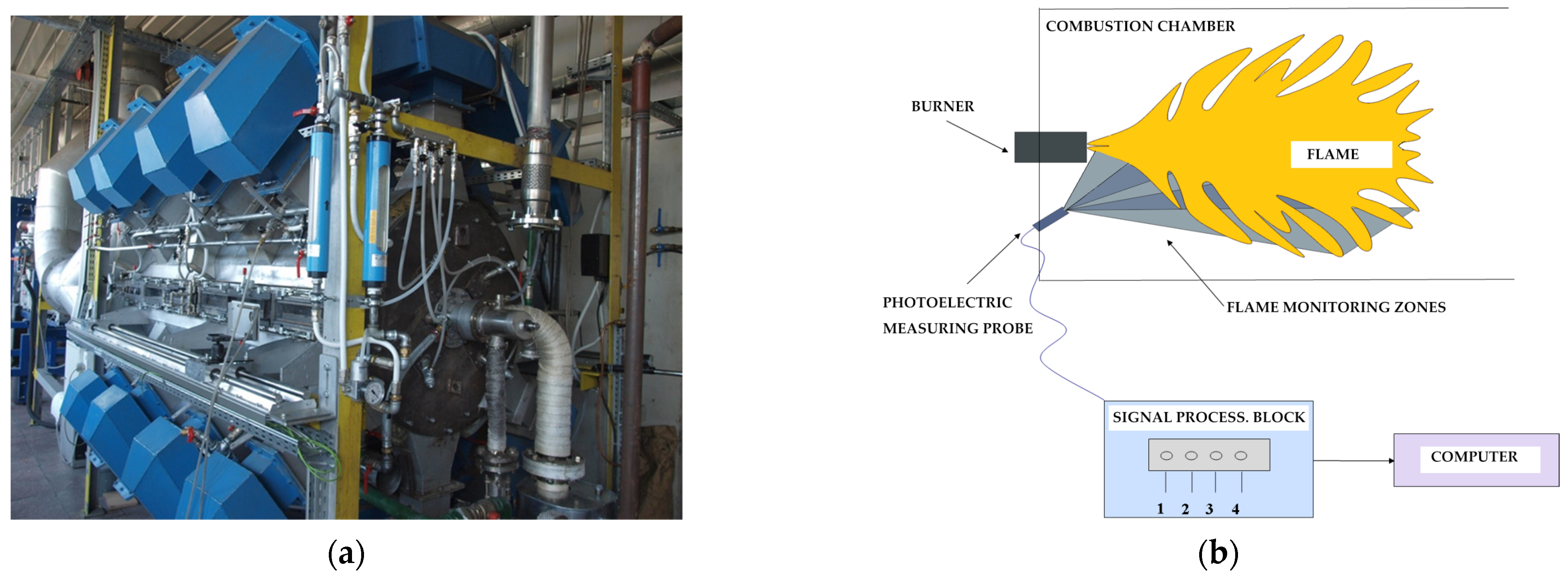
Figure 1. (a) Measurement station and (b) schematic of the fiber-optic flame monitoring system.
Energies 17 00212 g001
Figure 2. Changes in flame intensity for 100% pulverized coal.
Energies 17 00212 g002
Figure 3. Flame intensity of individual probe channels for the first signal.
Energies 17 00212 g003
Figure 4. Correlation graphs of variables from channels 1–4 for measurement signal numbers 1 (a), 2 (b), 3 (c), 4 (d), 5 (e), and 6 (f).
Energies 17 00212 g004
Figure 5. Changes in flame intensity for the measurement signals of flame no. 7 with the determined trend function: y = 0.1402 + 0.3013 × 10⁻⁵ × x, R2 = 0.9594.
Energies 17 00212 g005
Figure 6. Changes in flame intensity for the measurement signals of flame no. 13 with the determined trend function: y = 0.9005 − 0.3274 × 10⁻⁵ × x, R2 = 0.9628.
Energies 17 00212 g006
Figure 7. Changes in flame intensity for the measurement signals of flame no. 19 with the determined trend function: y = 0.1096 × exp(0.8397 × 10⁻⁵ × x), R2 = 0.9202.
Energies 17 00212 g007
Figure 8. Changes in flame intensity for the measurement signals of flame no. 25 with the determined trend function: y = 0.7068 × exp(−0.7057 × 10⁻⁵ × x), R2 = 0.7615.
Energies 17 00212 g008
Figure 9. One-step prediction of the time series of changes in the flame intensity for the signals of flame no. 1: (a) measurement data with forecast; (b) measurement data in the range of 0−25000 ms and forecast in the range of 25001−30000 ms.
Energies 17 00212 g009
Figure 10. Fuzzy rule table for ANFIS model for multi-class classification variant.
Energies 17 00212 g010
Figure 11. Input membership functions in the ANFIS model.
Energies 17 00212 g011
Figure 12. Binary classification confusion matrices for the models: (a) ANFIS_FCM, (b) ANFIS_GP, and (c) ANFIS_SC.
Energies 17 00212 g012
Figure 13. Comparison of model testing results for binary classification of flame states.
Energies 17 00212 g013
Figure 14. Multi-class classification confusion matrices for models: (a) ANFIS_FCM and (b) ANFIS_GP.
Energies 17 00212 g014
Figure 15. Comparison of ANFIS_GP model classification results for flame states 0–5.
Energies 17 00212 g015
Figure 16. Comparison of classification accuracy of different fuzzy models.
Energies 17 00212 g016
Table 1. Selected statistical values for measurement signals 1–6.
Flame
Signal Number
FuelMinimum ValueMaximum ValueAverage ValueRoot Mean Square ValueStandard
Deviation
Coefficient of Variation [%]
1_channel1100%
pulverized coal
0.04130.13450.07850.07980.014318.2172
1_channel20.15740.41860.25780.25780.039515.4895
1_channel30.16960.41530.25240.25450.032812.98,04
1_channel40.23910.50000.32520.32690.032710.0675
2_channel10.02820.08490.04030.04070.005714.1211
2_channel20.11840.29460.15200.15290.015710.3252
2_channel30.13150.29820.16560.16630.01539.2587
2_channel40.18500.41300.22810.22890.01928.4217
3_channel10.06660.12500.09500.09530.00697.2773
3_channel20.25850.42850.32770.32820.01855.6302
3_channel30.27130.43470.33640.33690.01855.4973
3_channel40.34410.58660.42380.42470.02776.5352
4_channel180%
pulverized coal
with 20%
biomass
0.04000.10690.07730.07760.017021.9923
4_channel20.18430.34770.25970.26040.01927.3835
4_channel30.19480.39040.27820.27920.02418.6503
4_channel40.24180.60340.34700.35000.046213.3201
5_channel10.03960.10360.06480.06580.011417.5534
5_channel20.15220.34610.21910.22140.032214.6776
5_channel30.16040.33890.22340.22540.030013.4112
5_channel40.20170.41860.27100.27310.033812.4776
6_channel10.01540.07440.02840.02910.006221.9591
6_channel20.06820.22270.10330.10460.016015.5302
6_channel30.07110.21420.10510.10620.014814.0935
6_channel40.08590.25060.12520.12630.017113.6292
Table 2. Fit measures for selected flame intensity measurement signals.
Flame
Signal Number
SSER2RMSENumber
of Coefficients
164240.02500.16172
7475.31250.95940.04402
13512.78890.96280.04572
19949.73690.92020.06222
2520100.76150.09042
Table 3. Fit measures for selected flame intensity measurement signals.
Flame
Signal Number
Model
Parameter
ValueStandard ErrorStatistics t
1Constant value–6.7588 × 10−76.4078 × 10−6–0.1055
AR{1}0.99993.3437 × 10−52.9903 × 10⁻⁴
MA{1}–0.57750.0015–373.9257
Variance5.6424 × 10−51.4437 × 10−7390.8195
7Constant value9.9979 × 10−83.7923 × 10−60.0264
AR{1}0.99920.8581 × 10−41.1644 × 10⁻⁴
MA{1}–0.50580.0020–251.4473
Variance1.3065 × 10−53.0852 × 10−8423.4724
13Constant value–1.0662 × 10−74.0297 × 10−6–0.0265
AR{1}0.99928.6789 × 10−51.1513 × 10⁻⁴
MA{1}–0.54810.0019–281.4230
Variance1.7332 × 10−54.4769 × 10−8387.1379
19Constant value1.4874 × 10−61.5015 × 10−60.9906
AR{1}11.7996 × 10−55.5567 × 10−4
MA{1}–0.57870.0015–375.9948
Variance3.1232 × 10−61.6239 × 10−8192.3328
25Constant value3.2273 × 10−72.0362 × 10−60.1585
AR{1}0.99991.9903 × 10−550240
MA{1}–0.40670.0015–265.2504
Variance2.9296 × 10−61.4723 × 10−8198.9732
Table 4. Selected quality measures of binary classification of flame states.
ModelSensitivityPrecisionF1 ScoreAccuracy [%]
ANFIS_FCM0.960.860.9190.43
ANFIS_GP0.950.960.9595.46
ANFIS_SC0.970.850.9189.96
Table 5. Selected quality measures of multi-class classification of flame states.
ModelClassSensitivityPrecisionF1 ScoreAccuracy [%]
ANFIS_FCM00.161.000.2867.07
10.820.360.50
20.210.400.28
30.870.870.87
40.970.980.98
51.000.990.99
ANFIS_GP00.271.000.4379.08
10.910.520.66
20.680.740.71
30.940.930.93
40.941.000.97
51.001.001.00
Disclaimer/Publisher’s Note: The statements, opinions and data contained in all publications are solely those of the individual author(s) and contributor(s) and not of MDPI and/or the editor(s). MDPI and/or the editor(s) disclaim responsibility for any injury to people or property resulting from any ideas, methods, instructions or products referred to in the content.